Abstract
With the increasing penetration of wind and photovoltaic (PV) power in modern power systems, accurate power forecasting has become crucial for ensuring grid stability and optimizing dispatch strategies. This study focuses on multiple wind farms and PV plants, where three deep learning models—Long Short-Term Memory (LSTM), Bidirectional LSTM (Bi-LSTM), and a hybrid Transformer–BiLSTM model—are constructed and systematically compared to enhance forecasting accuracy and dynamic responsiveness. First, the predictive performance of each model across different power stations is analyzed. The results reveal that the LSTM model suffers from systematic bias and lag effects in extreme value ranges, while Bi-LSTM demonstrates advantages in mitigating time-lag issues and improving dynamic fitting, achieving on average a 24% improvement in accuracy for wind farms and a 20% improvement for PV plants compared with LSTM. Moreover, the Transformer–BiLSTM model significantly strengthens the ability to capture complex temporal dependencies and extreme power fluctuations. Experimental results indicate that the Transformer–BiLSTM consistently delivers higher forecasting accuracy and stability across all test sites, effectively reducing extreme-value errors and prediction delays. Compared with Bi-LSTM, its average accuracy improves by 19% in wind farms and 35% in PV plants. Finally, this paper discusses the limitations of the current models in terms of multi-source data fusion, outlier handling, and computational efficiency, and outlines directions for future research. The findings provide strong technical support for renewable energy power forecasting, thereby facilitating efficient scheduling and risk management in smart grids.
1. Introduction
With the intensifying challenges of global climate change [1,2,3], the development of green and low-carbon energy [4,5,6] has become a strategic priority in national energy transitions. As essential components of renewable energy, wind [7,8] and solar power [9,10] are gaining a steadily increasing share in the global energy mix due to their environmental sustainability and abundant resources. China, as a leading country in installed capacity of wind and photovoltaic (PV) power, is actively promoting the large-scale integration and application of renewable energy, which plays a critical role in achieving carbon peak and carbon neutrality goals [11,12]. However, the inherent intermittency and volatility of renewable power generation significantly increase the complexity of grid scheduling, posing challenges to the security, stability, and economic efficiency of power systems. Consequently, accurate and efficient forecasting of wind and PV power has become a prominent research focus.
A considerable body of research has explored power forecasting for renewable energy, with machine learning and deep learning methods receiving significant attention due to their ability to effectively capture complex nonlinear relationships in time-series data. Traditional forecasting approaches primarily include linear and nonlinear models. For instance, the Autoregressive Moving Average (ARMA) model [13], as a representative linear method, captures correlations in time series by assuming linear dependencies among past observations and has been applied to power load and generation forecasting to some extent. However, such models struggle to represent the intricate dynamic characteristics embedded in power series. On the other hand, nonlinear models such as the Autoregressive Conditional Heteroskedasticity (ARCH) [14] model can describe volatility clustering and variance shifts, yet conventional time series approaches generally rely on strict stationarity assumptions and are highly sensitive to initial conditions. These limitations hinder their ability to address the inherent nonstationary, strong fluctuations, and multi-scale nonlinear features prevalent in renewable power generation, thereby constraining both forecasting accuracy and practical applicability.
Unlike traditional models that rely on strict stationarity assumptions, machine learning approaches can automatically extract features from historical data with fewer prior constraints, making them particularly suitable for handling high-dimensional, nonlinear, and complex dynamic relationships. Artificial neural networks [15] (ANNs) and other deep learning frameworks outperform conventional methods by capturing nonlinear patterns in the data. For example, Mabel et al. [16] developed an ANN model with a backpropagation algorithm and achieved promising results in wind power forecasting by adjusting the network architecture. Gao et al. [17] introduced a CNN–GRU-based ultra-short-term wind power forecasting model using multi-channel signals derived from multivariate input data of wind farms. Their approach leveraged CNNs to extract both global and local features, yielding high computational accuracy and robustness in wind power forecasting. Jang et al. [18] proposed a photovoltaic forecasting model based on satellite imagery and a support vector machine (SVM) scheme, where SVM effectively learned from large-scale satellite datasets, demonstrating its strong capability in data processing. Nevertheless, traditional machine learning methods often depend heavily on handcrafted features, which limits their applicability mainly to short-sequence forecasting. To achieve more powerful feature extraction and improve prediction accuracy over long sequences, deep learning models with memory mechanisms are indispensable. In this regard, the Long Short-Term Memory (LSTM) network has been introduced to retain relevant information across extended sequences and effectively address long-term dependencies, thereby becoming one of the most important deep learning models for time series forecasting.
The Long Short-Term Memory (LSTM) network, proposed by Hochreiter and Schmidhuber in 1997 [19], addresses the gradient vanishing and exploding issues that hindered the training of traditional recurrent neural networks (RNNs) on long sequences. By incorporating a gating mechanism, LSTM effectively retains and selectively updates memory cells, enabling it to capture long-term dependencies in sequential data. Owing to these advantages, LSTM has been widely applied in power forecasting. For instance, Zhou et al. [20] developed an LSTM-based point forecasting model for wind power, leveraging its strong memory capability to establish correlations between past and future data, thereby improving forecasting accuracy. Similarly, Alguhi and Al-Shaalan [21] proposed an LSTM network for solar irradiance and wind speed forecasting, which enabled effective prediction of wind and photovoltaic power. Nevertheless, LSTM relies solely on past information in long-sequence forecasting. To alleviate this limitation, Graves and Schmidhuber [22] modified the architecture and introduced the Bidirectional LSTM (Bi-LSTM), which employs forward and backward LSTM layers to utilize both past and future temporal information simultaneously. The superiority of Bi-LSTM over LSTM has been validated in various studies. For example, Siami-Namini et al. [23] demonstrated that Bi-LSTM can achieve better forecasting performance by performing additional training on the data. Liu et al. [24] further proposed an AC-BiLSTM model for ultra-short-term power load forecasting, achieving satisfactory results. However, Bi-LSTM remains largely dependent on local temporal features, and its memory of early information is still limited when handling long sequences. As the number of time steps increases, critical information may gradually weaken or be lost, leading to degraded performance in long-term forecasting tasks
The Transformer architecture, proposed by Vaswani et al. [25] in 2017, leverages a self-attention mechanism to capture global dependencies within data sequences, enabling efficient processing of large-scale datasets. Since its introduction, Transformer has been widely applied across various domains. For instance, Li et al. [26] developed a Transformer-based approach for short-term voltage stability assessment, where the self-attention mechanism was employed to learn critical features in the data. Their results demonstrated that the Transformer-based method exhibited robustness under class imbalance and data noise conditions. Similarly, Islam et al. [27] analyzed the applications and impacts of Transformer in natural language processing (NLP), computer vision (CV), multimodal learning, audio and speech processing, and signal processing, highlighting its cross-domain adaptability. Overall, Transformer is capable of parallel processing long sequences while selectively attending to relevant sequence elements without the need for fixed-order dependencies, establishing itself as a leading model in both natural language processing and time series forecasting.
At present, the key challenge in renewable power forecasting lies in achieving high accuracy under complex and fluctuating meteorological conditions, particularly on medium- to long-term scales. Most existing approaches focus primarily on short-term forecasting or rely on simplified assumptions, which limits their ability to comprehensively characterize the nonstationary and multi-scale dynamics inherent in wind and photovoltaic (PV) power generation processes. For power systems with a high share of renewable energy, reliable medium- to long-term forecasting is crucial for enhancing grid dispatch flexibility, facilitating renewable energy integration, and ensuring secure and stable system operation. To address this need, this study proposes a Transformer–BiLSTM model that combines the sequential dependency modeling capability of LSTM with the global attention mechanism of Transformer. This hybrid framework provides a more robust and accurate forecasting tool under complex conditions, offering valuable support for the planning and operation of power systems with high renewable energy penetration.
In this study, we propose a Transformer–BiLSTM model for renewable power forecasting. The model integrates the global dependency modeling capability of Transformer with the bidirectional temporal feature extraction strength of Bi-LSTM, thereby providing a more effective representation of the nonstationary and multi-scale dynamics inherent in wind and photovoltaic (PV) power series. Empirical results based on multiple wind farms and PV plants demonstrate that the proposed model achieves substantially higher forecasting accuracy than existing methods: for wind farm data, the average accuracy improves by 43% and 19% compared with LSTM and Bi-LSTM, respectively; for PV plant data, the corresponding improvements are 55% and 35%.
Based on the above context, the main contributions of this study are as follows: (1). A hybrid forecasting model combining Transformer and Bi-LSTM (Transformer–BiLSTM) is proposed, which simultaneously captures global dependencies and bidirectional temporal features; (2). The study introduces a renewable power forecasting model capable of accurately predicting power generation over a one-month horizon.
The structure of this paper is organized as follows: Section 2 presents the methodology, including data preprocessing procedures, factor analysis methods, the construction of forecasting models and evaluation metrics, as well as the configuration of the experimental platform. Section 3 details the results and discussion, including analyses of key influencing factors, forecasting performance across different regions, and an in-depth discussion of their implications. Section 4 concludes the study by summarizing the main contributions and proposing directions for future research, as well as potential applications in renewable energy management.
2. Methods
The methodology adopted in this study can be divided into four parts: data preprocessing, influencing factor analysis, model training, and model forecasting, as illustrated in Figure 1 (modified based on the reference [28]).
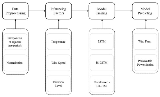
Figure 1.
Flowchart of the research methodology (modified based on the reference [28]).
In the data preprocessing stage, interpolation was performed using a method that combines adjacent time periods with historical data from the same period, followed by normalization. This approach addresses missing values and standardizes the variable ranges, thereby ensuring data quality and facilitating model convergence. The influencing factor analysis primarily evaluates key variables, such as temperature, wind speed, solar radiation, precipitation, and relative humidity, to gain a deeper understanding of the most influential predictors. The model training stage involves the construction and training of three models—LSTM, Bi-LSTM, and Transformer-BiLSTM—on the preprocessed datasets. Finally, in the model forecasting stage, the trained models are applied to predict the power output of wind farms and photovoltaic (PV) plants in Jiangxi Province. The forecasting results are then evaluated to assess each model’s effectiveness in capturing the dynamics of renewable energy power generation.
2.1. Data Preprocessing
The renewable power generation data used in this study were obtained from actual measurements at various renewable energy plants in Jiangxi Province, spanning the period from 2021 to 2023, with a total of 1095 days. The corresponding meteorological data were sourced from ERA5, covering the same time period as the measured power data. The actual power output of each plant from 2021 to 2023 is illustrated in Figure 2 and Figure 3.
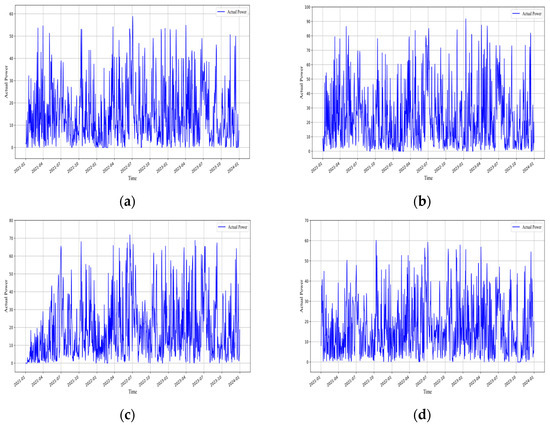
Figure 2.
Daily power plot of all wind farms in Jiangxi Province. (a) Daily power plot of Wind Farm 1 in Jiangxi Province. (b) Daily power plot of Wind Farm 2 in Jiangxi Province. (c) Daily power plot of Wind Farm 3 in Jiangxi Province. (d) Daily power plot of Wind Farm 4 in Jiangxi Province.
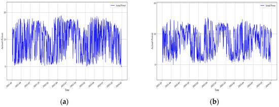
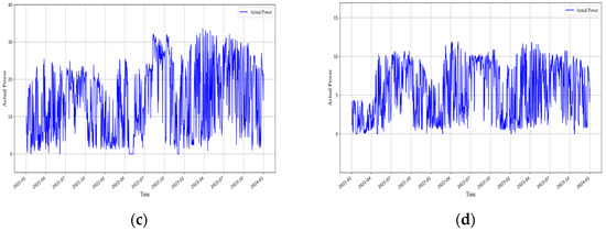
Figure 3.
Daily power plot of all photovoltaic plants in Jiangxi Province. (a) Daily power plot of Photovoltaic Plant 1 in Jiangxi Province. (b) Daily power plot of Photovoltaic Plant 2 in Jiangxi Province. (c) Daily power plot of Photovoltaic Plant 3 in Jiangxi Province. (d) Daily power plot of Photovoltaic Plant 4 in Jiangxi Province.
Analysis of the measured power data from photovoltaic and wind power plants in Jiangxi Province indicates that both exhibit pronounced nonstationary and volatility. Photovoltaic power shows a clear daily periodicity, rising during the day with increasing solar irradiance and approaching zero at night. It is also influenced by meteorological conditions such as cloud cover and precipitation, resulting in short-term, sharp fluctuations. Seasonal peak differences are significant, and even within the same season, power output varies randomly across different days (Figure 3). Wind power, on the other hand, exhibits intermittency and strong variability driven by wind speed and other meteorological factors, encompassing both short-term high-frequency fluctuations and long-term changes in mean and variance (Figure 2). These characteristics underscore the complexity of forecasting photovoltaic and wind power, further highlighting the necessity of employing deep learning models to capture nonlinear features and both short- and long-term dependencies.
During the data preprocessing phase of this study, a series of steps were undertaken to address quality and consistency issues in both meteorological and power generation data, including duplicate record removal, missing value handling, outlier detection, and data imputation. First, duplicate meteorological and power records at the same time points were removed. Second, missing meteorological data were treated using a combination of interpolation over adjacent time periods and historical same-period estimates, while missing power generation data were supplemented using historical averages or linear interpolation. Third, unreasonable meteorological observations and power values outside operational ranges were identified and excluded by applying appropriate thresholds. Finally, for partially missing power generation information, interpolation was additionally performed with reference to observations from neighboring plants. After completing these steps, all input features were normalized using Min-Max normalization to map values to the [0, 1] range, thereby eliminating dimensional discrepancies and enhancing model training stability. These preprocessing procedures effectively improved data completeness, accuracy, and usability, providing a reliable foundation for subsequent analysis and modeling.
2.2. Influencing Factor Analysis
In the field of renewable energy generation, wind and photovoltaic (PV) power outputs are highly sensitive to meteorological conditions, such as wind speed, air temperature, solar radiation, and humidity, which significantly affect their generation characteristics. Accurately identifying and quantifying the influence of these meteorological factors is crucial for optimizing power forecasting models, enhancing the scientific basis of dispatch strategies, and ensuring stable grid operation. Considering the multidimensional, nonlinear, and noisy nature of meteorological data, this study employs the Random Forest (RF) model [29,30] to quantify the importance of meteorological factors. This approach not only handles high-dimensional features while mitigating overfitting, but also provides intuitive feature importance metrics that reflect the contribution of each meteorological variable to power variations, thereby offering solid data support for subsequent feature selection and structural design of forecasting models.
The Random Forest (RF) model makes predictions by aggregating multiple decision trees generated from different training subsets, each obtained through bootstrap sampling of the original dataset. During node splitting, the model searches for the optimal split within a randomly selected subset of features, enhancing model diversity and generalization capability. For classification tasks, predictions are aggregated by majority voting, whereas for regression tasks, the mean value of the outputs from all trees is used, thereby improving overall accuracy and robustness. The formulas involved in the Random Forest scoring model are as follows:
where denotes the total number of decision trees in the Random Forest; represents the prediction of sample by the tree; is the importance score of the feature in the tree; denotes the set of all nodes in the tree; is the weight of node ; is the mean squared error (MSE) before splitting node ; are the MSEs after splitting the left and right child nodes of node ; is the average importance of the feature across all trees; and is the normalized importance of the feature.
2.3. Power Generation Forecasting
To evaluate the effectiveness of the models, the dataset was chronologically divided into training and testing sets, with the last 30 days reserved for testing. This approach prevents data leakage from the future, ensuring the realism of the forecasting scenario, while leveraging over three years of historical data to fully capture long-term trends and seasonal patterns between meteorological variables and power output. Additionally, using the most recent month as the testing set allows for the assessment of model generalization under current meteorological conditions and operational states, and facilitates intuitive comparative analysis of model performance across historical and future periods.
2.3.1. Construction of Forecasting Models
This study employs a hybrid model combining a Transformer encoder with Bidirectional LSTM (Bi-LSTM) to enhance feature representation and comprehensively capture bidirectional dependencies in long-term time series. The model first uses the Transformer encoder to extract global correlations from the multivariate time series data, and then applies Bi-LSTM to simultaneously model forward and backward dynamic patterns, thereby strengthening the representation of complex temporal relationships. After multiple layers of feature processing, the model produces the forecasted output, effectively improving prediction accuracy.
The hybrid model combining Transformer and Bi-LSTM leverages the strengths of both architectures in time series modeling. The Transformer component employs a multi-head self-attention mechanism to address global dependencies in long-term forecasting and allows parallel processing of the entire sequence, significantly improving feature extraction efficiency. Its encoder consists of multi-head self-attention layers and feedforward neural networks (FFN), enabling the capture of multi-scale dependencies across different subspaces and performing nonlinear mapping of features. The Bi-LSTM component, on the other hand, models the sequence in both forward and backward directions, complementing the Transformer’s limitations in capturing local temporal details. This synergistic modeling of global and local dependencies enhances overall prediction accuracy.
In the self-attention mechanism, the dependencies between each time step in the sequence can be computed as follows:
where is query vector; is key vector; is value vector; and is dimension of the key vector.
The multi-head attention mechanism extends the self-attention mechanism in parallel across multiple subspaces, thereby enhancing the model’s capability to represent different sub-features. In the Transformer encoder, each layer leverages multi-head attention to capture global features from the sequence and applies a feedforward network (FFN) to perform nonlinear mapping and enhancement of these features, improving their representational effectiveness. To compensate for the model’s lack of inherent positional information, the Transformer introduces positional encoding, embedding temporal position information into the input features using sine and cosine functions, allowing the model to capture the sequential order. The formulation is as follows:
where denotes the position in the sequence, is the feature dimension index, represents the model’s hidden layer dimension, and 10,000 is the scaling factor used for distributing positional frequencies.
After extracting global features with the Transformer encoder, these features are fed into the Bidirectional Long Short-Term Memory (Bi-LSTM) layer. Bi-LSTM is an enhanced recurrent neural network (RNN) composed of forward and backward LSTM layers, capable of simultaneously capturing dependencies in both directions of a time series, thereby providing a more comprehensive modeling of temporal features. Each LSTM unit combines memory cells with gating mechanisms, such as the forget gate, input gate, and output gate, effectively retaining important information while suppressing irrelevant or redundant information. The update process of a single LSTM unit can be described by the following gating equations:
where represent the forget gate, input gate, and output gate, respectively; denotes the current input; is the hidden state from the previous time step; is the memory cell state; denotes the Sigmoid activation function; is the hyperbolic tangent function; and represents the Hadamard element-wise product.
The update process of Bi-LSTM is performed jointly by two directional LSTMs. On one hand, the forward LSTM sequentially updates the forget gate, input gate, candidate memory cell, cell state, and hidden state from time step to , producing the forward hidden sequence . On the other hand, the backward LSTM performs the same updates in reverse order, from time step to , yielding the backward hidden sequence . Finally, the forward and backward hidden states are concatenated or summed at each time step to form an output representation that incorporates bidirectional temporal dependencies, enabling comprehensive modeling of contextual features in the time series.
We propose a Transformer-BiLSTM model, whose architecture is illustrated in Figure 4. First, the input multivariate time series data are embedded through a linear layer, and positional information is injected via a positional encoding layer to preserve the sequential order. Subsequently, the Transformer encoder models the global dependencies in the input data and extracts global features. These features are then fed into the Bidirectional LSTM (Bi-LSTM) layer, capturing dependencies in both forward and backward temporal directions. Finally, the Bi-LSTM outputs are mapped to the forecasted results through a linear layer, enabling the synergistic modeling of long-term dependencies and local temporal features, thereby improving prediction accuracy and generalization capability.
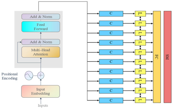
Figure 4.
Architecture of the Transformer-BiLSTM Model.
2.3.2. Evaluation Metrics of Forecasting Models
Analyzing the forecasting results of renewable energy generation (wind and photovoltaic power) is challenging due to the large amount of data spanning different time periods. To quantitatively evaluate the overall performance and predictive accuracy of the models, four evaluation metrics were employed in this study: Root Mean Square Error (RMSE), Mean Absolute Error (MAE), Explained Variance Score (EVS), and Coefficient of Determination (R2). These metrics are used to identify the optimal forecasting model, and the corresponding formulas are as follows:
where denotes the number of samples, and represent the actual and predicted values, respectively.
2.3.3. Goodness-of-Fit Evaluation of Forecasting Models
To ensure a robust evaluation of the forecasting models for renewable energy generation, this study employs four key metrics [31]: Root Mean Square Error (RMSE), Mean Absolute Error (MAE), Explained Variance Score (EVS), and Coefficient of Determination (R2) to assess model goodness-of-fit. Table 1 lists the corresponding thresholds for each metric and categorizes model performance into four levels: “Great,” “Good,” “Satisfactory,” and “Unsatisfactory”. These thresholds not only facilitate the quantification of predictive accuracy but also enable comprehensive comparisons of forecasting performance across different feature domains.

Table 1.
Evaluation Criteria for Forecasting Model Metrics.
Each metric provides a specific and valuable assessment of model performance, collectively forming a comprehensive framework for evaluating forecasting accuracy. RMSE and MAE measure the absolute magnitude of errors, with thresholds set at 50% of the standard deviation to effectively distinguish acceptable errors from significant deviations. This distinction is particularly important in renewable energy power forecasting, where large errors may indicate potential issues. RMSE is more sensitive to large errors, whereas MAE serves as a measure of overall error, reducing the influence of outliers. EVS evaluates the relative variance of prediction errors, facilitating intuitive comparisons across different regions and verifying model stability and applicability in diverse environments. The coefficient of determination, R2, represents the proportion of data variance explained by the model; a value exceeding 0.5 generally indicates that the model captures the primary trends in the data. By integrating these metrics, model performance can be comprehensively assessed from the perspectives of absolute error, relative error, and goodness-of-fit, thereby aiding in the selection of the most reliable forecasting method.
2.4. Experimental Platform
This study employed the deep learning framework PyTorch 1.11.0 for model development, with experimental code implemented in Python 3.9.10. Data processing and experiments were conducted on a Windows platform. The Transformer–BiLSTM model was optimized using the Adam optimizer, and hyperparameters such as sliding window length, learning rate, and number of training epochs were tuned via Bayesian optimization to achieve optimal performance. Detailed experimental configurations are summarized in Table 2.
Table 2.
Experimental Configuration.
3. Results
3.1. Results of Influencing Factors
To identify the most relevant factors affecting the power output of the two types of renewable energy, this study employed a Random Forest model to evaluate the importance of various meteorological variables for wind and photovoltaic (PV) power generation. For wind power, the analysis focused on wind speed, temperature, humidity, and precipitation. The results in Table 3 indicated that wind speed had the greatest influence, with an importance score of 0.71, followed by temperature with a score of 0.16, while humidity and precipitation had minimal impact, scoring only 0.06 and 0.07, respectively. For PV power, solar radiation was the dominant factor, with an importance score of 0.88, whereas the other three meteorological variables had negligible effects, each scoring no more than 0.05. Based on the importance scores of influencing factors for the two energy types, wind power forecasting utilized wind speed and temperature as input variables, while PV power forecasting relied solely on solar radiation.
Table 3.
Importance Scores of Influencing Factors for Different Renewable Energy Power Plants.
3.2. Forecasting Results of the Models
This section primarily evaluates and compares the forecasting performance of three different models—LSTM, Bi-LSTM, and Transformer-BiLSTM—applied to various types of renewable energy generation. The analysis focuses on prediction accuracy and the correlation with actual values using both numerical metrics and visualizations, including scatter plots and time series graphs. A comprehensive assessment of model performance across different renewable energy types is thereby conducted.
3.2.1. Forecasting Results of Wind Power Generation
Based on the LSTM forecasting results for each wind farm (Figure 5) and the corresponding performance metrics (Table 4), it is evident that the model exhibits certain systematic deviations and fluctuations across all wind farms. In Jiangxi Wind Farm 1 and Wind Farm 4, the predicted values deviate significantly from the actual values in multiple periods, with a general tendency of underestimation in high-value ranges and overestimation in low-value ranges, reflecting the model’s poor adaptability to non-stationary conditions. Moreover, the predicted values at several power peaks are considerably lower than the actual ones, with the maximum gap being particularly prominent, indicating insufficient reliability in forecasting maximum output. In Jiangxi Wind Farm 2, the model consistently underestimates during high-power stages, showing a conservative forecasting pattern. While this reduces the risk of overestimation, it also significantly underestimates the farm’s maximum generation capacity and scheduling value under strong wind conditions. In Jiangxi Wind Farm 3, the dynamic consistency between the predicted curve and the actual values is unstable, exhibiting both obvious “lagging effects” and premature responses. This suggests that the model’s reaction to temporal feature changes is either overly sensitive or insufficiently stable, leading to pronounced time-shift errors. Overall, the LSTM model still shows considerable room for improvement in trend capturing, peak response, and dynamic stability.
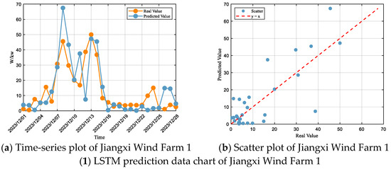
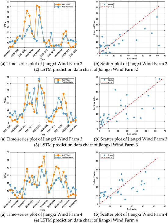
Figure 5.
LSTM Forecasting Plots for Each Wind Farm.
Table 4.
Evaluation of LSTM Model Metrics for Each Wind Farm.
According to the fitting evaluation criteria, the performance of the LSTM model at Jiangxi Wind Farm 1 falls within the “Unsatisfactory” range, with an R2 of 0.48 indicating weak explanatory power. The RMSE and MAE account for 71% and 49% of the standard deviation, respectively, which also places the model in the satisfactory range. At Jiangxi Wind Farm 2, the performance is within the “Unsatisfactory” range, with an R2 of only 0.43, while the RMSE and MAE represent 74% and 47% of the standard deviation, respectively, thereby positioning the model in the “Unsatisfactory” range. At Jiangxi Wind Farm 3, the performance is also “Unsatisfactory”, with an R2 of merely 0.40, and the RMSE and MAE accounting for 76% and 77% of the standard deviation, respectively, which again classifies the model as “Unsatisfactory”. At Jiangxi Wind Farm 4, the performance remains in the “Unsatisfactory” range, with an R2 of only 0.37, while the RMSE and MAE account for 78% and 65% of the standard deviation, respectively, thereby also categorizing the model as “Unsatisfactory”.
Based on the Bi-LSTM prediction results for each wind farm (Figure 6) and the corresponding performance metrics (Table 5), it can be observed that the overall performance of this model has improved compared to LSTM, yet certain deviations and fluctuations still exist. At Jiangxi Wind Farm 1, although irregular oscillations persist, the model shows significant improvement over LSTM; the overall fluctuation trend aligns with the actual values, and while both high and low power regions are slightly underestimated, the vertical spread of extreme errors is reduced, indicating enhanced error control. At Jiangxi Wind Farm 2, the underestimation in high power regions remains, but errors are noticeably smaller than those of LSTM, reflecting better extreme value capture, whereas the overestimation in low power regions is not significantly mitigated. For Jiangxi Wind Farm 3, the output trend is generally consistent with the actual values, with improved lag effects; high power regions are better predicted with smaller errors, although some periods still exhibit over-response and premature prediction, and the fluctuation amplitude can even exceed that of LSTM. At Jiangxi Wind Farm 4, the predicted curve closely follows the actual values, with a marked reduction in lag and stronger dynamic response, though slight underestimation in high power regions and overestimation in low power regions still exist. Overall, the Bi-LSTM model outperforms LSTM in trend tracking, extreme value capture, and error control, but systematic deviations in high and low power regions remain to be further optimized.
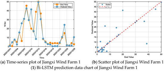
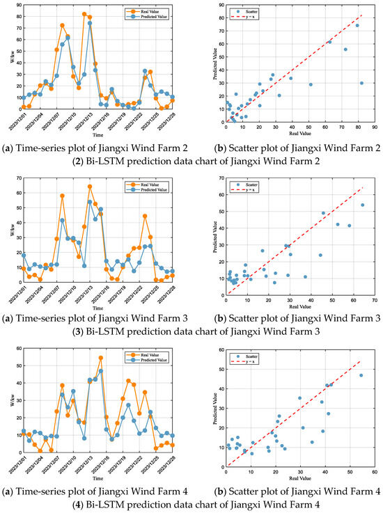
Figure 6.
Bi-LSTM Forecasting Plots for Each Wind Farm.
Table 5.
Evaluation of Bi-LSTM Model Metrics for Each Wind Farm.
According to the model fit evaluation criteria, the performance of the Bi-LSTM model at Jiangxi Wind Farm 1 falls within the “Satisfactory” range, with an R2 of 0.65, and RMSE and MAE accounting for 58% and 31% of the standard deviation, respectively. At Jiangxi Wind Farm 2, the model performance is also within the “Satisfactory” range, with an R2 of 0.71, and RMSE and MAE accounting for 53% and 34% of the standard deviation, respectively. For Jiangxi Wind Farm 3, the performance remains in the “Satisfactory” range, with an R2 of 0.68, and RMSE and MAE accounting for 55% and 45% of the standard deviation, respectively. At Jiangxi Wind Farm 4, the model similarly achieves “Satisfactory” performance, with an R2 of 0.61, and RMSE and MAE accounting for 61% and 49% of the standard deviation, respectively.
Based on the Transformer-BiLSTM prediction results for each wind farm (Figure 7) and the corresponding performance metrics (Table 6), it is evident that this model outperforms both LSTM and Bi-LSTM in terms of dynamic response, trend tracking, and error control. At Jiangxi Wind Farm 1, the irregular oscillations almost disappear, and the predicted trend closely aligns with the actual values, with high-power intervals matching well and only slight overestimation in low-power intervals, accompanied by minor errors. At Jiangxi Wind Farm 2, the predictions fit the actual values well in high-power intervals, with significantly enhanced extreme-value capturing ability, and only minor overestimation occurs in low-power intervals. For Jiangxi Wind Farm 3, the predicted trend is consistent with actual values, the lag effect is notably improved, high-power intervals show excellent performance with small errors, and low-power intervals exhibit slight overestimation within a controlled range. At Jiangxi Wind Farm 4, the predicted trend aligns with actual values, dynamic response is markedly improved, errors in high-power intervals are significantly reduced, and overestimation in low-power intervals remains within a manageable range. Overall, the Transformer-BiLSTM model achieves precise tracking of power fluctuations and effective error suppression across all wind farms, demonstrating superior generalization and predictive capability.
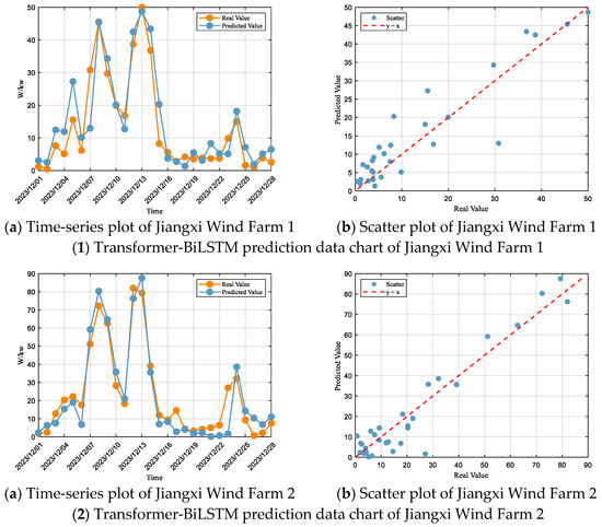
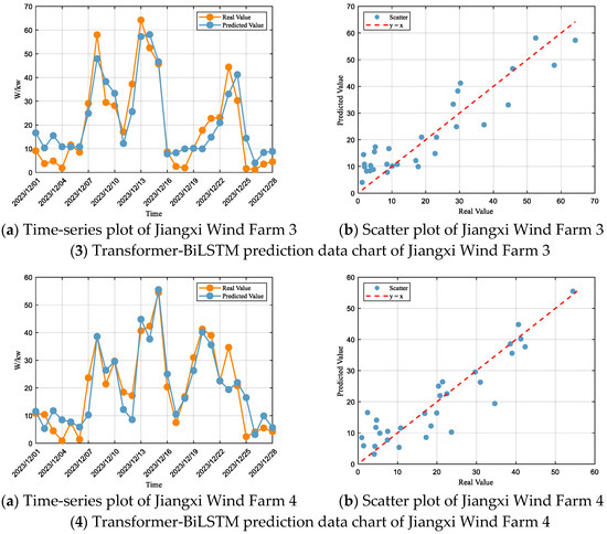
Figure 7.
Transformer-BiLSTM Forecasting Plots for Each Wind Farm.
Table 6.
Evaluation of Transformer-BiLSTM Model Metrics for Each Wind Farm.
According to the model evaluation criteria, the Transformer-BiLSTM model demonstrates “Great” performance at Jiangxi Wind Farm 1, with an R2 of 0.84, and RMSE and MAE accounting for 39% and 28% of the standard deviation, respectively, placing the model within the “Great” range. At Jiangxi Wind Farm 2, the performance is also rated as “Great,” with an R2 of 0.90, and RMSE and MAE representing 31% and 24% of the standard deviation, respectively. For Jiangxi Wind Farm 3, the model shows “Great” performance in terms of R2 (0.84), while RMSE and MAE account for 40% and 34% of the standard deviation, placing it within the “Satisfactory” range. At Jiangxi Wind Farm 4, the model achieves “Great” performance, with an R2 of 0.82, and RMSE and MAE corresponding to 41% and 31% of the standard deviation, respectively.
Overall, in the forecasting experiments for wind farms, the Transformer–BiLSTM model achieved significantly lower RMSE and MAE compared to LSTM and Bi-LSTM, indicating its superior capability in capturing short-term fluctuations and reducing overall prediction errors in wind power. Additionally, the model attained an average R2 of 0.85, demonstrating strong performance in fitting the overall trend of wind power generation. Moreover, the relatively high Explained Variance Score (EVS) indicates that the model can better account for the variance in power sequences, maintaining robust performance under varying meteorological conditions. These results suggest that the Transformer–BiLSTM model not only enhances forecasting accuracy but also offers greater practical value for grid dispatch and renewable energy integration.
3.2.2. Forecasting Results of Photovoltaic Power Generation
Based on the LSTM prediction results for the photovoltaic (PV) plants (Figure 8) and their performance metrics (Table 7), it can be observed that the model exhibits certain systematic deviations and fluctuations across different PV sites. At Jiangxi PV Plant 1, the predicted values deviate significantly from the actual values during multiple periods, accompanied by frequent oscillations. High-power intervals are generally underestimated, while low-power intervals tend to be overestimated, showing a “high-low inversion” pattern, indicating that the model struggles to adapt to rapid power changes and non-stationary fluctuations. At Jiangxi PV Plant 2, the high-power outputs are almost consistently underestimated, reflecting a conservative prediction behavior that reduces the risk of overestimation but limits revenue assessment and dispatch optimization. Jiangxi PV Plant 3 shows irregular fluctuations in the predicted curve, with dynamic matching varying over time. Both noticeable lag effects and premature responses occur, indicating that the model’s reaction to temporal changes is unstable, leading to significant time-shift errors. For Jiangxi PV Plant 4, the overall trend aligns with the actual values, but errors are amplified near peaks and troughs; high-power segments are underestimated, and low-power segments are slightly overestimated, reflecting insufficient generalization capability in extreme regions and the difficulty of accurately capturing extreme operational states.
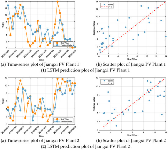
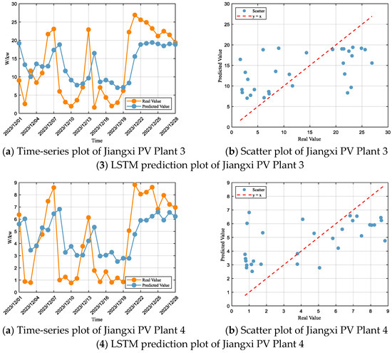
Figure 8.
Time-series plots of LSTM predictions for all PV plants.
Table 7.
Evaluation of LSTM model performance for each PV plant.
According to the goodness-of-fit evaluation criteria, the LSTM model’s performance for Jiangxi PV Plant 1 falls within the “Unsatisfactory” range, with an R2 of 0.38, and RMSE and MAE accounting for 76% and 62% of the standard deviation, respectively, placing the model in the “Unsatisfactory” category. For Jiangxi PV Plant 2, the performance is also “Unsatisfactory”, with an R2 of 0.40, and RMSE and MAE accounting for 76% and 55% of the standard deviation. Jiangxi PV Plant 3 exhibits “Unsatisfactory” performance as well, with an R2 of 0.30, and RMSE and MAE accounting for 82% and 68% of the standard deviation. Finally, for Jiangxi PV Plant 4, the model’s performance remains “Unsatisfactory”, with an R2 of 0.34, and RMSE and MAE accounting for 80% and 68% of the standard deviation.
Based on the Bi-LSTM prediction results for the Jiangxi PV Plants (Figure 9) and their performance metrics (Table 8), it can be observed that the model achieves improved prediction accuracy compared with LSTM, but certain systematic biases remain. For Jiangxi PV Plant 1, although predictions are better than LSTM, high-power intervals are still underestimated while low-power intervals tend to be overestimated. For Jiangxi PV Plant 2, the underestimation in high-power intervals has been significantly alleviated and errors substantially reduced, yet overestimation persists in low-power intervals. Jiangxi PV Plant 3 shows good dynamic alignment with actual values and overall trend consistency, but some interval-specific deviations remain, with high-power intervals still underestimated and low-power intervals slightly overestimated. For Jiangxi PV Plant 4, high-power underestimation and low-power overestimation are improved compared to LSTM, but deviations persist. Overall, the Bi-LSTM model outperforms LSTM in prediction accuracy and dynamic response, yet systematic biases in extreme power intervals still require further optimization.
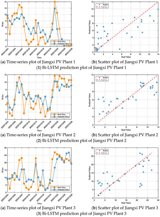
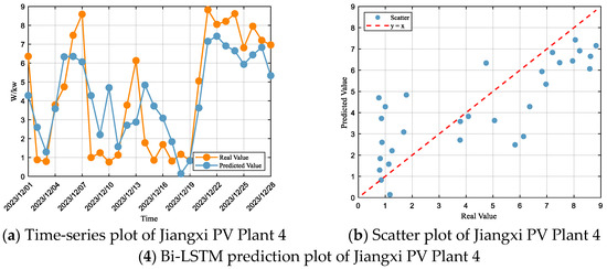
Figure 9.
Time-series plots of Bi-LSTM predictions for all PV plants.
Table 8.
Evaluation of Bi-LSTM model performance for each PV plant.
According to the fitting evaluation criteria, the Bi-LSTM model performs within the “Satisfactory” range at Jiangxi PV Plant 1, with an R2 of 0.54, and RMSE and MAE accounting for 66% and 53% of the standard deviation, respectively, which also place the model in the “Satisfactory” range. At Jiangxi PV Plant 2, the performance is also within the “Satisfactory” range, with an R2 of 0.63, and RMSE and MAE corresponding to 60% and 46% of the standard deviation, respectively, thus meeting the satisfactory standard. At Jiangxi PV Plant 3, the model’s performance falls into the “Unsatisfactory” range, with an R2 of 0.46, and RMSE and MAE representing 73% and 53% of the standard deviation, respectively, which classify the model as “Unsatisfactory”. At Jiangxi PV Plant 4, the model again performs within the “Satisfactory” range, with an R2 of 0.60, and RMSE and MAE accounting for 62% and 52% of the standard deviation, respectively, thereby also placing the model in the “Satisfactory” range.
Based on the Transformer-BiLSTM prediction results for each PV plant (Figure 10) and their corresponding performance metrics (Table 9), it can be observed that the model demonstrates both high adaptability and accuracy across different plants. At Jiangxi PV Plant 1, the prediction errors remain low in both high- and low-power ranges, indicating stable forecasting performance. At Jiangxi PV Plant 2, the overestimation issue in the low-power range is significantly alleviated, with a noticeable reduction in deviations from the actual values. At Jiangxi PV Plant 3, the predicted curve closely follows the variations in the actual values, with markedly enhanced dynamic responsiveness, while both high-value underestimation and low-value overestimation are effectively mitigated. At Jiangxi PV Plant 4, the errors associated with high-power underestimation and low-power overestimation are also substantially reduced. Overall, the Transformer-BiLSTM model achieves error suppression and accuracy enhancement in power prediction across all plants, exhibiting strong generalization ability and stability.
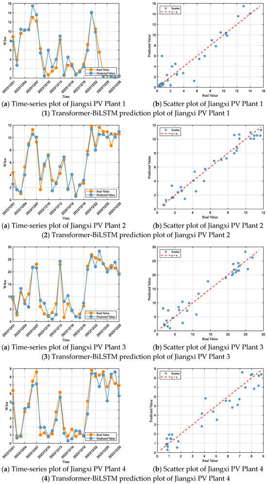
Figure 10.
Time-series plots of Transformer-BiLSTM predictions for all PV plants.
Table 9.
Evaluation of Transformer-BiLSTM model performance for each PV plant.
According to the fitting evaluation criteria, the performance of the Transformer-BiLSTM model at Jiangxi photovoltaic power station 1 falls within the “Great” range, with an R2 of 0.88, while the RMSE and MAE account for 34% and 22% of the standard deviation, respectively, also placing the model in the “Great” range. At Jiangxi photovoltaic power station 2, the performance is also within the “Great” range, with an R2 of 0.94, and the RMSE and MAE accounting for 24% and 19% of the standard deviation, respectively, also placing the model in the “Great” range. At Jiangxi photovoltaic power station 3, the performance is within the “Great” range, with an R2 of 0.92, and the RMSE and MAE accounting for 28% and 21% of the standard deviation, respectively, also placing the model in the “Great” range. At Jiangxi photovoltaic power station 4, the performance is within the “Great” range, with an R2 of 0.91, and the RMSE and MAE accounting for 30% and 24% of the standard deviation, respectively, also placing the model in the “Great” range.
Overall, in the photovoltaic (PV) power forecasting experiments, the Transformer–BiLSTM model achieved significantly lower RMSE and MAE compared to LSTM and Bi-LSTM, indicating its superior capability in mitigating short-term deviations caused by fluctuations in solar irradiance and meteorological conditions. The model attained an average R2 of 0.91, demonstrating strong performance in capturing the overall trend of PV power output. Moreover, the relatively high Explained Variance Score (EVS) suggests that the model can effectively account for the variance in power sequences under varying weather conditions. These results indicate that the Transformer–BiLSTM model not only improves PV power forecasting accuracy but also exhibits enhanced robustness, providing significant value for grid dispatch and renewable energy integration.
3.3. Discussion
This study systematically compared the power prediction performance of wind farms and photovoltaic (PV) plants using three deep learning models: LSTM, Bi-LSTM, and Transformer-BiLSTM. The results indicate that with the evolution of model architectures, both prediction accuracy and dynamic response capability are significantly enhanced.
The traditional LSTM model generally underestimates power in high-output intervals and overestimates in low-output intervals, exhibiting a typical “high-low inversion” bias, which reflects its insufficient adaptability to non-stationary temporal fluctuations and extreme conditions. Additionally, the lag effect is evident in wind power predictions, resulting in inadequate capture of rapidly changing dynamics and limiting real-time forecasting reliability. The Bi-LSTM model, incorporating bidirectional temporal features, mitigates some systematic errors and lag issues, producing prediction curves that better align with actual fluctuations and reducing errors in extreme intervals. However, the model still exhibits occasional over-responses and residual deviations in high- and low-output intervals, indicating that its capability to model complex dynamics remains to be improved.
The Transformer-BiLSTM model combines the Transformer’s strength in capturing global dependencies with Bi-LSTM’s sequential feature modeling, demonstrating stronger generalization and prediction stability. Across all test sites, this model substantially improves the accuracy of extreme value responses, effectively overcomes lag effects, and achieves highly consistent tracking of power trends. Its ability to handle nonlinear and complex temporal data markedly surpasses the previous two models, providing a solid foundation for high-precision and reliable renewable energy power forecasting.
Despite these promising results, several limitations remain. First, the models primarily rely on limited historical meteorological and power data, without fully integrating multi-source heterogeneous information, which constrains their expressive capacity. Second, anomalies and missing data were not thoroughly addressed, potentially affecting prediction stability. Finally, the computational complexity of Transformer-BiLSTM limits its real-time application. Future research should focus on multimodal data fusion, anomaly detection and compensation mechanisms, and lightweight model design to enhance accuracy, robustness, and practicality.
In conclusion, the optimization of deep learning model architectures has significantly advanced renewable energy power forecasting, facilitating refined smart grid dispatch and risk management. Nevertheless, continuous exploration of more efficient and robust modeling solutions is required to meet the increasingly complex demands of practical applications.
4. Conclusions
This study systematically compared the performance of three deep learning models—LSTM, Bi-LSTM, and Transformer-BiLSTM—in forecasting the power output of wind farms and photovoltaic (PV) plants. The results demonstrate that continuous optimization of model architectures significantly enhances prediction accuracy and dynamic response capability. The conventional LSTM model exhibits notable biases and lag effects when handling non-stationary time series fluctuations and extreme power values, which adversely affect forecasting accuracy and real-time applicability. Bi-LSTM, by incorporating bidirectional temporal information, mitigates some of these errors and improves dynamic responsiveness, but systemic deviations in high- and low-power intervals remain. Transformer-BiLSTM, combining the Transformer’s ability to capture global dependencies with Bi-LSTM’s sequential feature learning, achieves higher predictive accuracy and stability across all sites, effectively overcoming lag effects and challenges associated with extreme value forecasting.
Despite these advances, there is room for improvement in data diversity utilization, anomaly handling, and computational efficiency. Future research should focus on multi-source data integration, anomaly compensation mechanisms, and lightweight model design to meet the high-accuracy and high-efficiency demands of renewable power forecasting in smart grids. Overall, this study provides an effective technical pathway for renewable energy power prediction, advancing its application in power system dispatch and risk management.
Author Contributions
Investigation, methodology, writing—original draft, and writing—review and editing, H.H. and W.H.; conceptualization, supervision, validation, and writing—review and editing, J.G.; data curation, software, writing—original draft, and funding acquisition, K.W.; data curation, software, visualization, and writing—original draft, W.Z. and Z.W. All authors have read and agreed to the published version of the manuscript.
Funding
This research was funded by the Key Science and Technology Project of State Grid Jiangxi Electric Power Co., Ltd.: Analysis of new energy output characteristics and research on power prediction improvement methods under extreme weather conditions (No.: 521820240013).
Data Availability Statement
The original contributions presented in this study are included in the article. Further inquiries can be directed to the corresponding author.
Conflicts of Interest
Authors Hao He, Wei He, Kang Wu, Weizhe Zhao, and Zijing Wan were employed by the company State Grid Jiangxi Electric Power Research Institute. The remaining authors declare that the research was conducted in the absence of any commercial or financial relationships that could be construed as a potential conflict of interest. The authors declare that this study received funding from the Key Science and Technology Project of State Grid Jiangxi Electric Power. The funder was not involved in the study design, collection, analysis, and interpretation of data, the writing of this article, nor the decision to submit it for publication.
References
- Abbass, K.; Qasim, M.Z.; Song, H.; Murshed, M.; Mahmood, H.; Younis, I. A Review of the Global Climate Change Impacts, Adaptation, and Sustainable Mitigation Measures. Environ. Sci. Pollut. Res. 2022, 29, 42539–42559. [Google Scholar] [CrossRef]
- Olabi, A.G.; Abdelkareem, M.A. Renewable Energy and Climate Change. Renew. Sustain. Energy Rev. 2022, 158, 112111. [Google Scholar] [CrossRef]
- Karl, T.R.; Trenberth, K.E. Modern Global Climate Change. Science 2003, 302, 1719–1723. [Google Scholar] [CrossRef]
- Xu, X.; Xia, J.; Hong, C.; Sun, P.; Xi, P.; Li, J. Optimization of Cooperative Operation of Multiple Microgrids Considering Green Certificates and Carbon Trading. Energies 2025, 18, 4083. [Google Scholar] [CrossRef]
- Li, B.; Cong, R.; Matsumoto, T.; Li, Y. Research on Different Energy Transition Pathway Analysis and Low-Carbon Electricity Development: A Case Study of an Energy System in Inner Mongolia. Energies 2025, 18, 3129. [Google Scholar] [CrossRef]
- Tian, J.; Yu, L.; Xue, R.; Zhuang, S.; Shan, Y. Global Low-Carbon Energy Transition in the Post-COVID-19 Era. Appl. Energy 2022, 307, 118205. [Google Scholar] [CrossRef] [PubMed]
- Zupok, S.; Chomać-Pierzecka, E.; Dmowski, A.; Dyrka, S.; Hordyj, A. A Review of Key Factors Shaping the Development of the U.S. Wind Energy Market in the Context of Contemporary Challenges. Energies 2025, 18, 4224. [Google Scholar] [CrossRef]
- Meng, W.; Yang, Z.; Yu, J.; Lin, X.; Yu, M.; Zhu, Y. Multi-Market Coupling Mechanism of Offshore Wind Power with Energy Storage Participating in Electricity, Carbon, and Green Certificates. Energies 2025, 18, 4086. [Google Scholar] [CrossRef]
- Caponi, R.; Vizza, D.; Bassano, C.; Del Zotto, L.; Bocci, E. Dynamic Comparative Assessment of Long-Term Simulation Strategies for an off-Grid PV–AEM Electrolyzer System. Energies 2025, 18, 4209. [Google Scholar] [CrossRef]
- Thom, D.; Bugała, A.; Bugała, D.; Czekała, W. Comprehensive Energy and Economic Analysis of Selected Variants of a Large-Scale Photovoltaic Power Plant in a Temperate Climate. Energies 2025, 18, 4198. [Google Scholar] [CrossRef]
- Wei, Y.-M.; Chen, K.; Kang, J.-N.; Chen, W.; Wang, X.-Y.; Zhang, X. Policy and Management of Carbon Peaking and Carbon Neutrality: A Literature Review. Engineering 2022, 14, 52–63. [Google Scholar] [CrossRef]
- Yang, P.; Peng, S.; Benani, N.; Dong, L.; Li, X.; Liu, R.; Mao, G. An Integrated Evaluation on China’s Provincial Carbon Peak and Carbon Neutrality. J. Clean. Prod. 2022, 377, 134497. [Google Scholar] [CrossRef]
- Hannan, E.J. The Estimation of the Order of an ARMA Process. Ann. Stat. 1980, 8, 1071–1081. [Google Scholar] [CrossRef]
- Bollerslev, T.; Engle, R.F.; Nelson, D.B. Chapter 49 Arch Models. In Handbook of Econometrics; Elsevier: Amsterdam, The Netherlands, 1994; Volume 4, pp. 2959–3038. [Google Scholar]
- Agatonovic-Kustrin, S.; Beresford, R. Basic Concepts of Artificial Neural Network (ANN) Modeling and Its Application in Pharmaceutical Research. J. Pharm. Biomed. Anal. 2000, 22, 717–727. [Google Scholar] [CrossRef]
- Carolin Mabel, M.; Fernandez, E. Analysis of Wind Power Generation and Prediction Using ANN: A Case Study. Renew. Energy 2008, 33, 986–992. [Google Scholar] [CrossRef]
- Gao, J.; Ye, X.; Lei, X.; Huang, B.; Wang, X.; Wang, L. A Multichannel-Based CNN and GRU Method for Short-Term Wind Power Prediction. Electronics 2023, 12, 4479. [Google Scholar] [CrossRef]
- Jang, H.S.; Bae, K.Y.; Park, H.-S.; Sung, D.K. Solar Power Prediction Based on Satellite Images and Support Vector Machine. IEEE Trans. Sustain. Energy 2016, 7, 1255–1263. [Google Scholar] [CrossRef]
- Hochreiter, S.; Schmidhuber, J. Long Short-Term Memory. Neural Comput. 1997, 9, 1735–1780. [Google Scholar] [CrossRef] [PubMed]
- Zhou, B.; Ma, X.; Luo, Y.; Yang, D. Wind Power Prediction Based on LSTM Networks and Nonparametric Kernel Density Estimation. IEEE Access 2019, 7, 165279–165292. [Google Scholar] [CrossRef]
- Alguhi, A.A.; Al-Shaalan, A.M. LSTM-Based Prediction of Solar Irradiance and Wind Speed for Renewable Energy Systems. Energies 2025, 18, 4594. [Google Scholar] [CrossRef]
- Graves, A.; Schmidhuber, J. Framewise Phoneme Classification with Bidirectional LSTM Networks. In Proceedings of the 2005 IEEE International Joint Conference on Neural Networks, 2005, Montreal, QC, Canada, 31 July–4 August 2005; Volume 4, pp. 2047–2052. [Google Scholar]
- Siami-Namini, S.; Tavakoli, N.; Namin, A.S. The Performance of LSTM and BiLSTM in Forecasting Time Series. In Proceedings of the 2019 IEEE International Conference on Big Data (Big Data), Los Angeles, CA, USA, 9–12 December 2019; pp. 3285–3292. [Google Scholar]
- Liu, F.; Liang, C. Short-Term Power Load Forecasting Based on AC-BiLSTM Model. Energy Rep. 2024, 11, 1570–1579. [Google Scholar] [CrossRef]
- Vaswani, A.; Shazeer, N.; Parmar, N.; Uszkoreit, J.; Jones, L.; Gomez, A.N.; Kaiser, Ł.; Polosukhin, I. Attention Is All You Need. In Proceedings of the 31st Conference on Neural Information Processing Systems (NIPS 2017), Long Beach, CA, USA, 4–9 December 2017; Curran Associates, Inc.: Red Hook, NY, USA, 2017; Volume 30. [Google Scholar]
- Li, Y.; Cao, J.; Xu, Y.; Zhu, L.; Dong, Z.Y. Deep Learning Based on Transformer Architecture for Power System Short-Term Voltage Stability Assessment with Class Imbalance. Renew. Sustain. Energy Rev. 2024, 189, 113913. [Google Scholar] [CrossRef]
- Islam, S.; Elmekki, H.; Elsebai, A.; Bentahar, J.; Drawel, N.; Rjoub, G.; Pedrycz, W. A Comprehensive Survey on Applications of Transformers for Deep Learning Tasks. Expert Syst. Appl. 2024, 241, 122666. [Google Scholar] [CrossRef]
- Zhang, G.; Li, H.; Wang, L.; Wang, W.; Guo, J.; Qin, H.; Ni, X. Research on Medium- and Long-Term Hydropower Generation Forecasting Method Based on LSTM and Transformer. Water 2024, 17, 5707. [Google Scholar] [CrossRef]
- Breiman, L. Random Forests. Mach. Learn. 2001, 45, 5–32. [Google Scholar] [CrossRef]
- Biau, G.; Scornet, E. A Random Forest Guided Tour. TEST 2016, 25, 197–227. [Google Scholar] [CrossRef]
- Pérez Sánchez, M.; Sánchez Romero, F.J.; Ramos, H.M.; López Jiménez, P.A. Calibrating a Flow Model in an Irrigation Network: Case Study in Alicante, Spain. Span. J. Agric. Res. 2017, 15, 28. [Google Scholar] [CrossRef]


Disclaimer/Publisher’s Note: The statements, opinions and data contained in all publications are solely those of the individual author(s) and contributor(s) and not of MDPI and/or the editor(s). MDPI and/or the editor(s) disclaim responsibility for any injury to people or property resulting from any ideas, methods, instructions or products referred to in the content. |
© 2025 by the authors. Licensee MDPI, Basel, Switzerland. This article is an open access article distributed under the terms and conditions of the Creative Commons Attribution (CC BY) license (https://creativecommons.org/licenses/by/4.0/).