Enhancing Thermal-Hydraulic Modelling in Dual Fluid Reactor Demonstrator: The Impact of Variable Turbulent Prandtl Number

Abstract

In response to the growing demand for advanced nuclear reactor technologies, this study addresses significant gaps in thermal-hydraulic modelling for dual fluid reactors (DFRs) by integrating Kays correlation to implement a variable turbulent Prandtl number in the Reynolds-averaged Navier–Stokes (RANS) simulations. Traditional approaches employing a constant value of the turbulent Prandtl number have proven inadequate, leading to inaccurate heat transfer predictions for low Prandtl number liquids. The study carefully selects the appropriate formula for the turbulent Prandtl number in the DFR context, enhancing the accuracy of thermal-hydraulic modelling. The simulations consider Reynolds numbers between 15,000 and 250,000, calculated based on the hydraulic diameters at different diameter pipes of the fuel and coolant loops. The molecular Prandtl number is equal to 0.025. Key findings reveal that uneven flow distributions within the fuel pipes result in variable temperature distribution throughout the reactor core, confirming earlier observations while highlighting significant differences in parameter values. These insights underscore the importance of model selection in CFD analysis for DFRs, revealing potential hotspots and high turbulence areas that necessitate further investigation into vibration and structural safety. The results provide a framework for improving reactor design and operational strategies, ensuring enhanced safety and efficiency in next-generation nuclear systems. Future work will apply this modelling approach to more complex geometries and flow scenarios to optimise thermal-hydraulic performance.

1. Introduction

The increasing demand for clean and sustainable energy sources has led to significant interest in advanced nuclear reactors [1], particularly within the framework of the GenIV nuclear systems [2]. The dual fluid reactor (DFR) concept has emerged as a promising candidate due to its distinct advantages over conventional designs, including salt fuel reactors [3]. Its ability to separate the fuel, flowing in many ceramic pipes, from a surrounding coolant enables operational flexibility, enhances safety, and optimises reactor efficiency [4,5]. In particular, the high operational temperatures of over 1200 K offer a potential pathway for electricity generation and hydrogen production, positioning DFR technology as a versatile energy solution [6,7].

One of the critical challenges facing the design of DFRs is the complex interaction between fluid flow and heat transfer, especially given the low Prandtl number of liquid metals typically used as coolants [7,8]. These interactions necessitate advanced thermal-hydraulic modelling to ensure precise temperature control and safety during reactor operations. Few thermal-hydraulic analyses were conducted previously for the DFR concept, for example, the work completed by Wang et al [9] to discuss the preliminary analysis of the full reactor or specific zones within the reactor in different configurations. The study used the k-ε model for the preliminary analysis of one zone in the DFR with a constant turbulent Prandtl number, which differs from the current model in which a variable turbulent Prandtl number is used.

Understanding the impact of property variations, such as temperature and density gradients, is vital for accurate thermal modelling in low Prandtl number fluids. A study by Toki et al. [10] demonstrated how property variations at supercritical pressures affect velocity and temperature profiles, providing insights into temperature correlations and transformation equations for such conditions. These findings align with the importance of addressing property variability in improving thermal predictions for systems like DFRs.

In our previous research, a comprehensive computational fluid dynamics (CFD) analysis of a small modular DFR was performed using the k-ω SST turbulence model, which employed a fixed value of the turbulent Prandtl number [11]. However, the study provides valuable insights into temperature and velocity distributions within the reactor core, identifying critical regions that influence reactor safety and efficiency. This standard turbulence model yielded acceptable accuracy in predicting fluid dynamics but revealed limitations in accurately capturing heat transfer phenomena, particularly under varying operational conditions. Shams et al. [12] introduced a new algebraic model targeting to increase prediction accuracy, but the model is not yet widely used in commercial solvers and has to be verified within different independent research communities.

A key limitation in the earlier analysis was using a constant value of the turbulent Prandtl number (Pr_t), which does not fully account for the variability in the thermal boundary layer, especially in highly turbulent flows [13]. The turbulent Prandtl number, which governs the relationship between momentum turbulent diffusivity and thermal diffusivity, can vary significantly under different flow regimes, and this variability has a direct impact on flow and heat transfer predictions. This is particularly relevant in nuclear reactor applications, where precise thermal management is crucial for efficiency and safety.

To address this limitation, the present study builds upon the foundation laid by our earlier work by introducing a variable turbulent Prandtl number, governed by the Kays correlation, into the k-ω SST model [14]. Kays correlation accounts for the varying turbulent Prandtl number in turbulent flows, offering a more nuanced approach to modelling heat transfer in systems involving low Prandtl number fluids such as liquid metals. Similar approaches have been applied in other domains, such as hypersonic boundary layer studies, where Huang et al. [15] demonstrated the importance of accounting for property variations to improve thermal predictions. By incorporating this refinement, we aim to improve the accuracy of thermal predictions, especially in regions where the heat transfer rate is critical to reactor operation and safety.

Introducing a variable turbulent Prandtl number is expected to yield more accurate temperature predictions within the reactor core, particularly in the thin thermal boundary layers where the standard model’s assumptions break down [16,17]. This study applies this improved model to the same modular DFR configuration used in our previous research [11], allowing for a direct comparison between the fixed and variable turbulent Prandtl number approaches. This comparison is crucial for understanding the impact of turbulence modelling refinements on reactor design, safety assessments, and operational strategies.

Furthermore, this work contributes to the broader field of nuclear reactor modelling by providing a validated approach for handling low Prandtl number flows. As advanced reactor designs, such as the DFR, continue to evolve, developing accurate, reliable CFD models will be essential for guiding the design process and ensuring that these reactors meet stringent safety and performance standards [5,9,18,19].

In summary, this study advances the state of thermal-hydraulic modelling for DFRs by incorporating a variable turbulent Prandtl number into the k-ω SST model, leveraging Kays correlation to improve heat transfer predictions. Similar to other reactor concepts [12], the results of this analysis not only enhance our understanding of thermal management in DFRs but also provide a valuable framework for future research aimed at optimising reactor design and ensuring safe and efficient operation in advanced nuclear systems.

2. Numerical Details

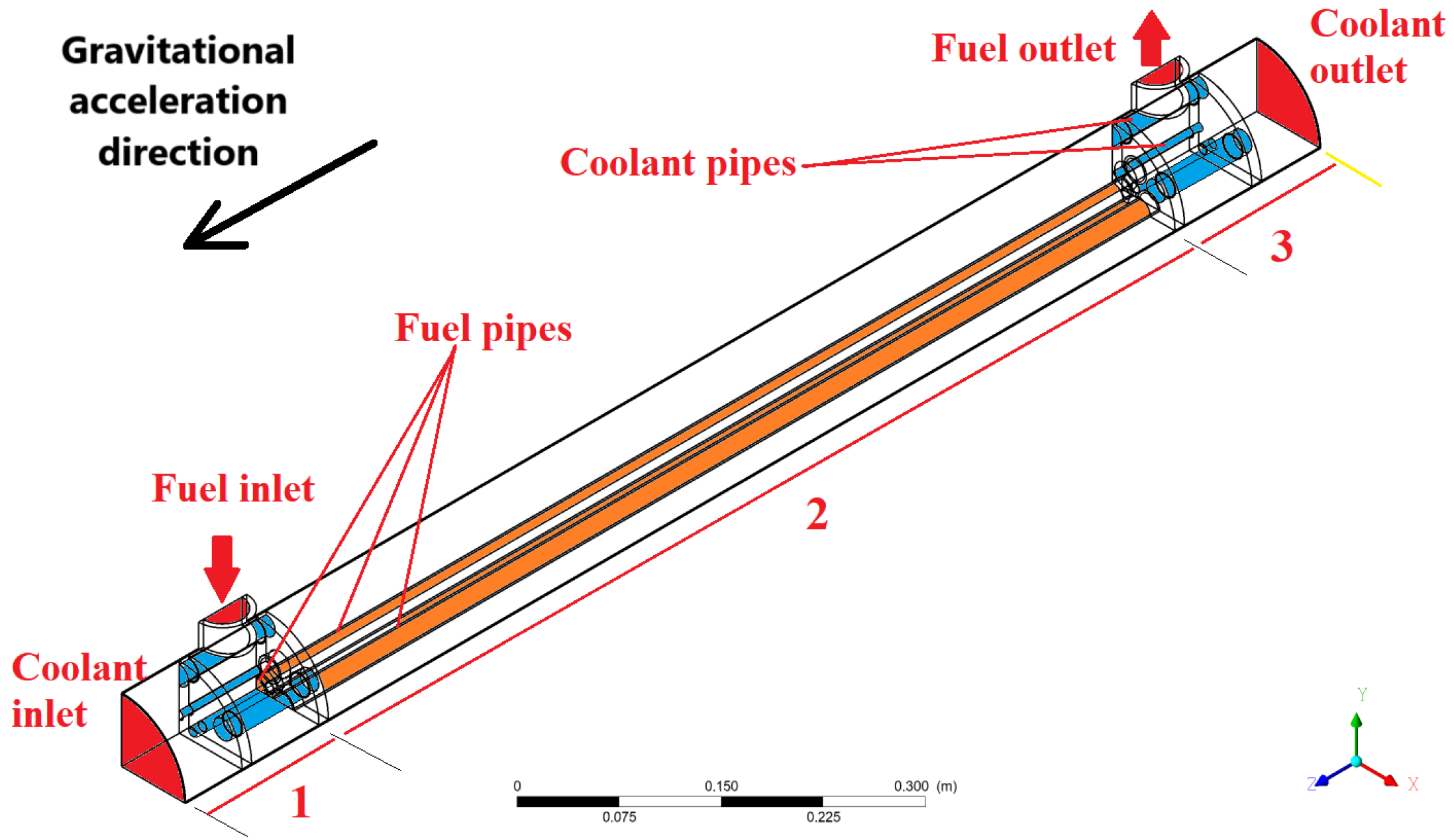
2.1. Description of Test Case

The mini demonstrator (MD) [11] is a simplified model designed to study the thermal hydraulics of the dual fluid reactor (DFR). It comprises two loops—fuel and coolant—each utilising molten lead to simulate the heat transfer processes within the DFR. This setup allows for in-depth analysis of the flow dynamics and heat transfer between the fuel and coolant regions, with several control and measuring devices ensuring accurate data acquisition.

In this study, both loops use molten lead to facilitate operational simplicity, avoiding the complexities associated with radioactive materials. Two magneto-hydraulic pumps (MHD) [20,21], commonly used in liquid metal-cooled reactors [22,23,24], are responsible for driving the flow in both loops. Each loop includes a storage tank with internal heaters, ensuring a reliable lead supply during operation.

The MD core, consisting of seven pipes with metallic liquid fuel, is divided into three main zones—distribution, middle core, and collection—provides insights into the heat transfer process (see Figure 1). The middle core zone is where most heat exchange occurs between the fuel pipes, surrounded by coolant. While detailed structural information and the whole computational model are available in our previous work, this paper focuses on the core’s thermal-hydraulic performance without addressing other components in the loop. Further details about the structural configuration and the specific operational mechanics of the MD can be found in our earlier publication [11].

Figure 2, Figure 3 and Figure 4 show the chosen planes (domain sections) for analysis. These planes include the longitudinal plane marked as A, the core transverse planes marked as B1–B4, and the Inlet/Outlet transverse planes denoted as C1 and C2. Figure 5 provides a detailed view beneath the demonstrator casing, highlighting the internal layout of the coolant and fuel domains within the distribution zone.

2.2. Governing Equations and Heat Transfer Model

The time-averaged mass, momentum, and energy conservation equations are

$${\displaystyle \frac{\partial \rho }{\partial t}}+{\displaystyle \frac{\partial \left(\rho U_i\right)}{\partial x_i}}=0$$

(1)

$${\displaystyle \frac{\partial \left(\rho U_i\right)}{\partial t}}+{\displaystyle \frac{\partial \left(\rho {U_{j}U}_i\right)}{\partial x_j}}=-{\displaystyle \frac{\partial P}{\partial x_i}}+{\displaystyle \frac{\partial }{\partial x_j}}\left[\mu \left({\displaystyle \frac{\partial U_i}{\partial x_j}}+{\displaystyle \frac{\partial U_j}{\partial x_i}}\right)-\rho \overline{u_i^{’}{u}_j^{’}}\right]+\rho g_i$$

(2)

$${\displaystyle \frac{\partial \left(\rho T\right)}{\partial t}}+{\displaystyle \frac{\partial \left(\rho U_{j}T\right)}{\partial x_j}}={\displaystyle \frac{\partial }{\partial x_j}}\left({\displaystyle \frac{\mu }{Pr}}{\displaystyle \frac{\partial T}{\partial x_j}}-\rho \overline{u_j^{’}{T}^{’}}\right)$$

(3)

where U_i, P, and T are the mean velocity components, pressure, and temperature, respectively. ρ is the fluid density, μ is the molecular dynamic viscosity, and Pr is the molecular Prandtl number. $g_i=\left(\mathrm{0,0},g\right)$ is the component of the gravitation acceleration vector in the i-th direction. The components of the modelled stress tensor are given by $-\rho \overline{u_i^{’}{u}_j^{’}}={\mu }_t\left({\displaystyle \frac{\partial U_i}{\partial x_j}}+{\displaystyle \frac{\partial U_j}{\partial x_i}}\right)-2/3\rho k{\delta }_{ij}$ with ${\mu }_t$ and k denoting the dynamic, turbulent viscosity and turbulent kinetic energy, respectively.

The Standard Gradient Diffusion Hypothesis (SGDH) model is applied for the prescription of the turbulent heat flux $-\overline{{u^{’}}_j{T}^{’}}$ in the energy Equation (3), utilising either constant or variable turbulent Prandtl number:

$$-\overline{{u^{’}}_j{T}^{’}}\cong {\displaystyle \frac{{\nu }_t}{P{r}_t}}{\displaystyle \frac{\partial T}{\partial x_j}}$$

(4)

with ${u^{’}}_j \text{and} T^{’}$, denoting the fluctuating velocity components and fluctuating temperature, respectively. The experimental and Direct Numerical Simulation (DNS) simulation studies [13,25] show that the turbulent Prandtl number attains values higher than unity in the low Prandtl flows. To address this, the empirical correlation by Kays [14] is adopted here:

$$P{r}_t=0.85+{\displaystyle \frac{0.7}{P{e}_t}}$$

(5)

with Pe_t denoting the turbulent Peclet number:

$$P{e}_t={\displaystyle \frac{{\nu }_t}{\nu }}Pr$$

(6)

In the formula (6), ν = μ/ρ is the molecular kinematic viscosity, and ν_t is the turbulent kinematic viscosity. The following section will show the model’s validation results.

Various k-ε and k-ω type turbulence models have been tested. However, the differences in the results were found to be small. Consequently, the k-ω SST model with active thermal buoyancy production term in the k-equation was selected for the flow simulation due to its robustness and superior performance in capturing flow characteristics near the walls and regions with adverse pressure gradients [26,27].

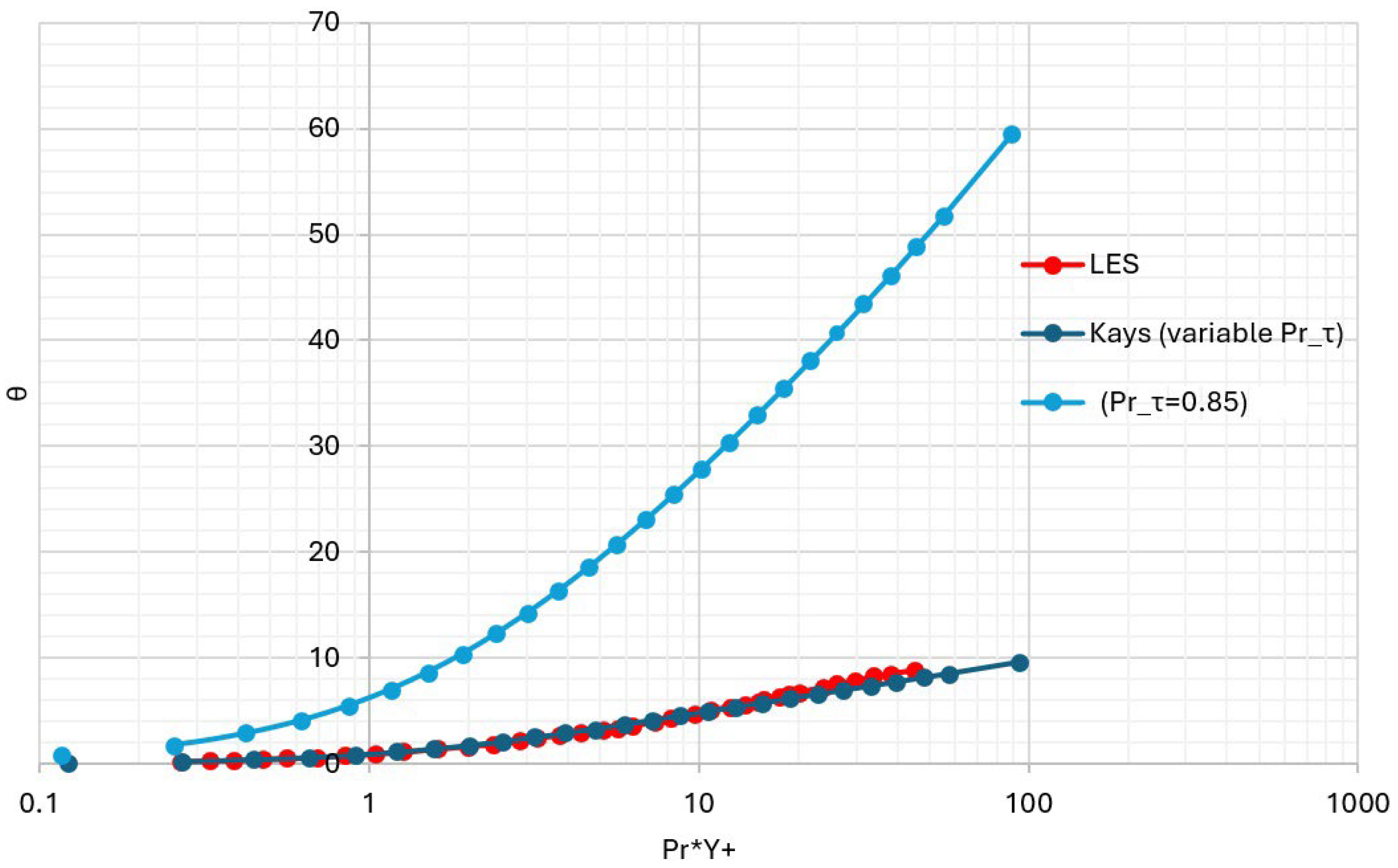
2.3. Validation of Heat Transfer Model

Due to the lack of available Direct Numerical Simulation (DNS) data that capture the turbulent Prandtl number within the specified range of Reynolds and Prandtl numbers, the Large Eddy Simulation (LES) data were utilised for thermal model validation in this study. The LES data were sourced from [14]. Knowing that $T_w$ is the mean wall temperature, and $T$ is the mean temperature; the non-dimensional mean temperature is defined as

$${\mathrm{\theta }}^{+}={\displaystyle \frac{T_w-T}{T_{\tau }}}$$

(7)

with $T_{\tau }$ the mean friction temperature:

$$T_{\tau }={\displaystyle \frac{q_w}{\rho c_p{\mathrm{u}}_{\tau }}}$$

(8)

In Equation (8), $q_w$ represents the heat flux, $c_p$ is the specific heat at constant pressure, and ${\mathrm{u}}_{\tau }$ is the friction velocity.

Figure 6 compares the non-dimensional temperature profiles for the simulation of fully developed channel flow at friction Reynolds number equal to $R{e}_{\tau }=2000$ [28]. The k-ω SST model simulation results are compared with reference LES, employing the constant (Pr_t = 0.85) and variable turbulent Prandtl numbers (Equation (5)). A significant difference between the LES and the k-ω SST results using the constant value of the turbulent Prandtl number is noted. However, there is a good agreement between Kay’s correlation (5) and LES. This is because the increased turbulent Prandtl number provided by Equation (5) leads to reduced turbulent heat flux in Equation (4).

These findings highlight the effectiveness of the SGDH model, combined with Kays’s correlation, for the estimation of the turbulent Prandtl number in the context of the MD case where heat transfer is a key factor.

2.4. Computational Details and Boundary Conditions

The computational model for the DFR demonstrator core comprises seven fuel pipes and twelve coolant pipes, with six large-diameter and six small-diameter pipes. Owing to the geometric symmetry of the core, only a quarter of the domain was simulated, optimising computational efficiency. The core’s design parameters were selected to align with those of the actual DFR to enhance the accuracy of experimental outcomes. The fuel and coolant pipes have wall thicknesses of 4 mm and 2 mm, respectively, and the entire solid structure is made of silicon carbide (SiC). In the simulation, the casing is assumed to be adiabatic to prevent heat exchange with the environment. Heat transfer within the pipe walls and separation discs was modelled in Fluent by defining temperature-dependent material properties, including a piece-wise linear function for specific heat capacity (C_p), a temperature-dependent function for thermal conductivity (κ), and a constant density (

Table 1. Thermo-physical properties of silicon carbide (solid structure).

Property	Interpolation/Value
Thermal Conductivity (W/(m K))	(611/(T − 115)) × 100
Density (kg/m3)	3210

). The physical properties of silicon carbide were obtained from Nilsson et al. [29]. Silicon carbide-specific heat was added to Ansys Fluent as piece-wise linear values (

Table 2. Specific heat of silicon carbide.

Temperature	Specific Heat (J/(kg K))
880	500
1060	625
1100	750
1220	1000
1280	1250

).

The properties of molten lead were incorporated using empirical correlations [30] appropriate for the relevant temperature ranges. The properties are summarised in

Table 3. Thermo-physical properties of liquid lead based on the temperature, T (K).

Property	Interpolation Function
Density (kg/m3)	11,463 − (1.32 × T)
Heat Capacity (J/(kg K))	175.1 − (4.961 × 10−2 × T) + (1.985 × 10−5 × T2) − (2.099 × 10−9 × T3) − (1.524 × 106 × T2)
Viscosity (Pa s)	EXP [(1032.2/T) − 7.6354]

.

The simulations have been performed with Ansys Fluent Solver ver. 2020 R1 [31]. The governing Equations (1)–(3) have been solved using the pressure-based segregated solver. The energy equation was activated to facilitate the prediction of the heat transfer phenomena. As mentioned, the k-ω SST model was employed for turbulence modelling. The value of the molecular Prandtl number was equal to 0.025. The variable turbulent Prandtl number (see Equation (5)) was introduced using the User Defined Function (UDF) functionality. The gravitational acceleration was activated towards the positive z-axis direction (Figure 1). Note that the MD, as well as the DFR design, is positioned vertically (along the z-direction) during operation, with the fuel inlet zone put closer to the ground than the fuel outlet zone.

Boundary conditions (

Table 4. Inlet boundary conditions for simulation of the Mini Demonstrator.

Name	Variable	Value	Unit
Fuel Inlet	Velocity magnitude	0.1	m/s
	Total temperature	1473	K
	Turbulent intensity	4	%
	The ratio of turbulent to molecular viscosity	100	-
Coolant Inlet	Velocity magnitude	0.5	m/s
	Total temperature	873	K
	Turbulent intensity	4	%
	The ratio of turbulent to molecular viscosity	100	-

) were set for fuel and coolant, similar to the previously published work [11]. Constant values of the velocity and temperature were imposed at the inlets. The fuel was introduced at an inlet velocity of 0.1 m/s and the coolant at 0.5 m/s, with atmospheric pressure conditions applied at the outlets. The turbulent intensity and the turbulent-to-molecular viscosities ratio were equal to 4% and 100, respectively. The MD outside casing boundary condition was considered adiabatic.

A sufficient quality grid was made with a y+ value of less than 5 in areas of significant heat transfer and velocity gradients, particularly at the interfaces of the fuel and coolant pipes.

A total of 25 million elements were generated to encompass the model’s quarter. Figure 7 shows the mesh resolution in the collection and distribution zones as well as a part of the coolant domain in the middle core zone and fuel in the fuel pipes.

A hybrid meshing approach was employed, using prismatic and tetrahedral cells tailored to specific regions. Inflation layers with high resolutions were applied in areas with high gradients of flow velocities, temperature changes, and heat transfer to ensure accurate predictions. Tetrahedral cells were used in complex regions where structured meshing was impractical. This approach optimised computational efficiency while capturing critical physical phenomena in high-gradient areas.

Numerical discretisation of the convective terms in the governing and transport equations was achieved using a second-order upwind scheme [32], with normalised residuals lowered to a 10⁻⁵ level.

The simulations were conducted in the Świerk Computing Centre at the National Centre for Nuclear Research (NCBJ) in Poland. A total of 25 compute nodes were utilised, each equipped with 40 processors, amounting to 1000 processors in total. This high-performance computing infrastructure facilitated the complex computations required for our study.

3. Results and Discussion

Due to the flow complexity in the distribution zone, the results obtained will first be shown in three x–y planes (see Figure 8). Figure 9 shows the outlines of fuel and cooler pipes in the x–y plane for comparison purposes in Figure 10 and Figure 11.

Figure 10 and Figure 11 show the contour plots of the velocity magnitude and static temperature in three x–y planes (Figure 8) of the distribution zone. The present results, obtained with variable turbulent Prandtl number (Equation (5)) and Pr = 0.025, are compared to the results obtained in previous work [11] with a constant value of the turbulent Prandtl (Pr_t = 0.85) and Pr = 0.025. The same turbulence model is employed in the present and previous studies, namely the k-ω SST model. The previous results obtained with the constant value of the turbulent Prandtl number (Figure 10, right) show a much stronger spreading of the incoming pipe flow in the inlet section due to a more uniform temperature distribution (Figure 11, right). Note that the liquid lead’s density, molecular viscosity, and heat capacity depend on the temperature field, as shown in Table 3. The increased temperature reduces the fluid density and viscosity, so changes the momentum transfer. The temperature becomes more uniform with the constant value of the turbulent Prandtl number due to the enhanced activity of the turbulent heat flux. Turbulence spreads the fluctuating momentum towards smaller scales. The simulation with the constant Pr_t interprets this process as intense temperature redistribution towards fluctuating temperature components. This significantly reduces the mean temperature gradient due to density and viscosity dependence on the temperature. This is not what happens in reality. In liquid metals, which are the low molecular Prandtl number fluids (Pr = 0.025), the fluctuating momentum does not significantly influence the fluctuating temperature fluxes. Molecular diffusion essentially governs the temperature field, while the flow is entirely turbulent [27]. The simulation results obtained with variable turbulent Prandtl number show much stronger mean velocity gradients (Figure 10, left) and the mean temperature gradients (Figure 11, left) in the distribution zone. This is due to the reduced effect of turbulent fluctuations on fluctuating energy fluxes. This results in reduced spreading of the high-velocity and high-temperature zones in Figure 10 (left) and Figure 11 (left) into the mixed-flow region. Consequently, the high-velocity and high-temperature flow can penetrate more effectively upwards towards one of the fuel pipes close to the bottom symmetry plane (Figure 10, Plane C, left) due to the buoyancy effect. It results in a much higher velocity than the case with a constant value of the turbulent Prandtl number (Figure 10, Plane C, right). Similar conclusions can be drawn by analysing the temperature field in Figure 11 (Plane C) The results show the importance of the variable turbulent Prandtl number on energy and momentum balance in MD.

In the following sections, the analysis of flow and temperature fields will be presented in simulation with variable turbulent Prandtl number.

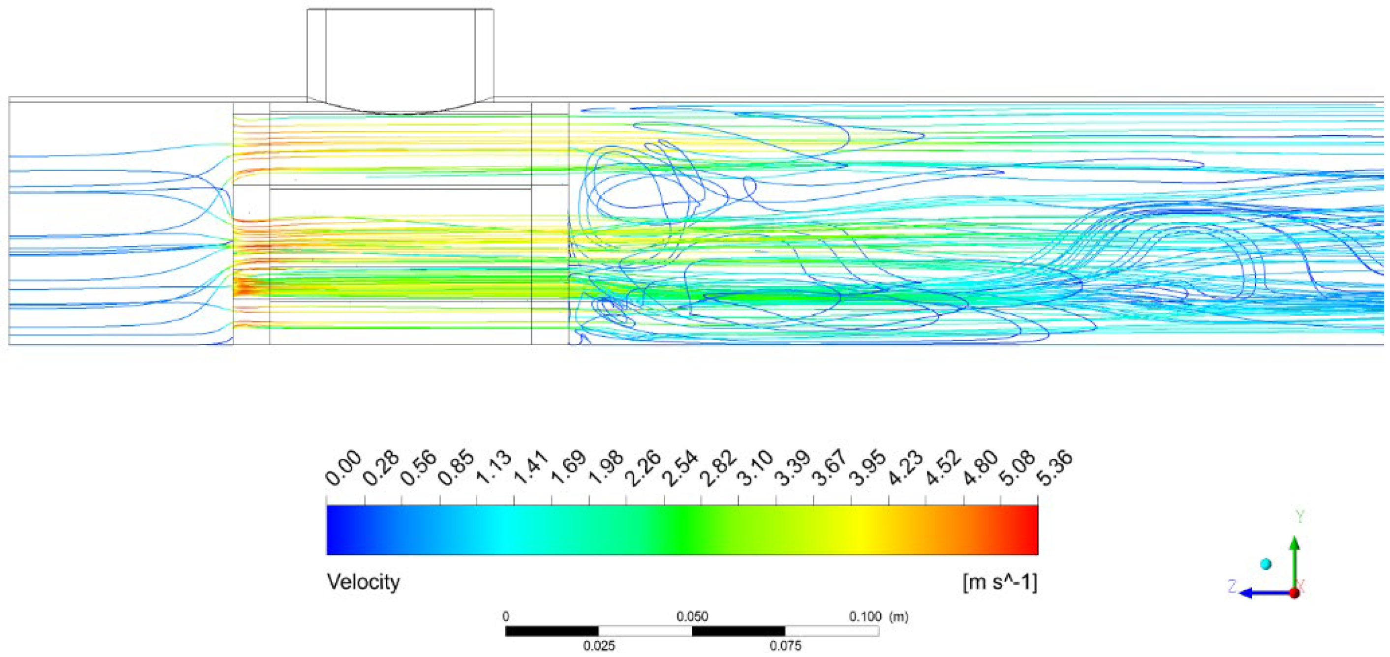
3.1. Velocity Field in the Fuel Region

As discussed, the fuel enters the distribution zone through two opposing inlets before proceeding into the middle core zone. Upon entering the middle part, the fuel encounters 12 coolant pipes, arranged as depicted in Figure 1. The coolant pipes, positioned directly in the path of the fuel, divide the flow into two distinct streams, as illustrated in Figure 12. This figure provides a cross-sectional view in the C-1 plane, previously depicted in Figure 4 and Figure 5. The interaction between the coolant pipes and the fuel flow results in a significant increase in fuel velocity within this region compared to other areas of the MD.

The fuel is directed through the fuel pipes in the core, necessitating a 90-degree shift in the flow direction. It gradually aligns with the direction of the fuel pipes, resulting in a diagonal flow pattern in the upper half of the zone, as illustrated in Figure 13. As discussed, this diagonal shape arises because the high temperature of the inlet fuel reduces its density and viscosity, causing the flow to move upward toward the fuel pipes without significant mixing with surrounding fluid elements.

In contrast, the flow in the lower half of the corner experiences significantly lower velocities. In this region, the flow separates from the stream and circulates within the zone’s lower half.

In the middle core zone, the fuel velocity varies across the pipes. Figure 14 illustrates the axial mean velocity component (denoted as w) in the B-1 plane (Figure 3) using an inverse rainbow colour scheme to represent the negative velocity components. The mass flow rates are also depicted in the figure in per cent of the total mass flow rate of the fuel. As shown, pipes #5 and #6 exhibit higher velocities, indicating a greater mass flow rate through these pipes. This is the result of flow non-uniformity in the fuel distribution zone, discussed earlier.

In the collection zone (Figure 15), the flow enters from the middle core region with higher velocities in pipes #5 and #6. The remaining pipes exhibit lower velocities (see also Figure 14). The elevated velocity in pipes #5 and #6 creates a jet-like effect. This concentrated flow strikes the separation disc at high velocity before redirecting toward the fuel exit, maintaining a relatively high speed between 0.1 and 0.2 m/s. The velocity increases at the fuel exit due to the reduced outlet area caused by flow separation.

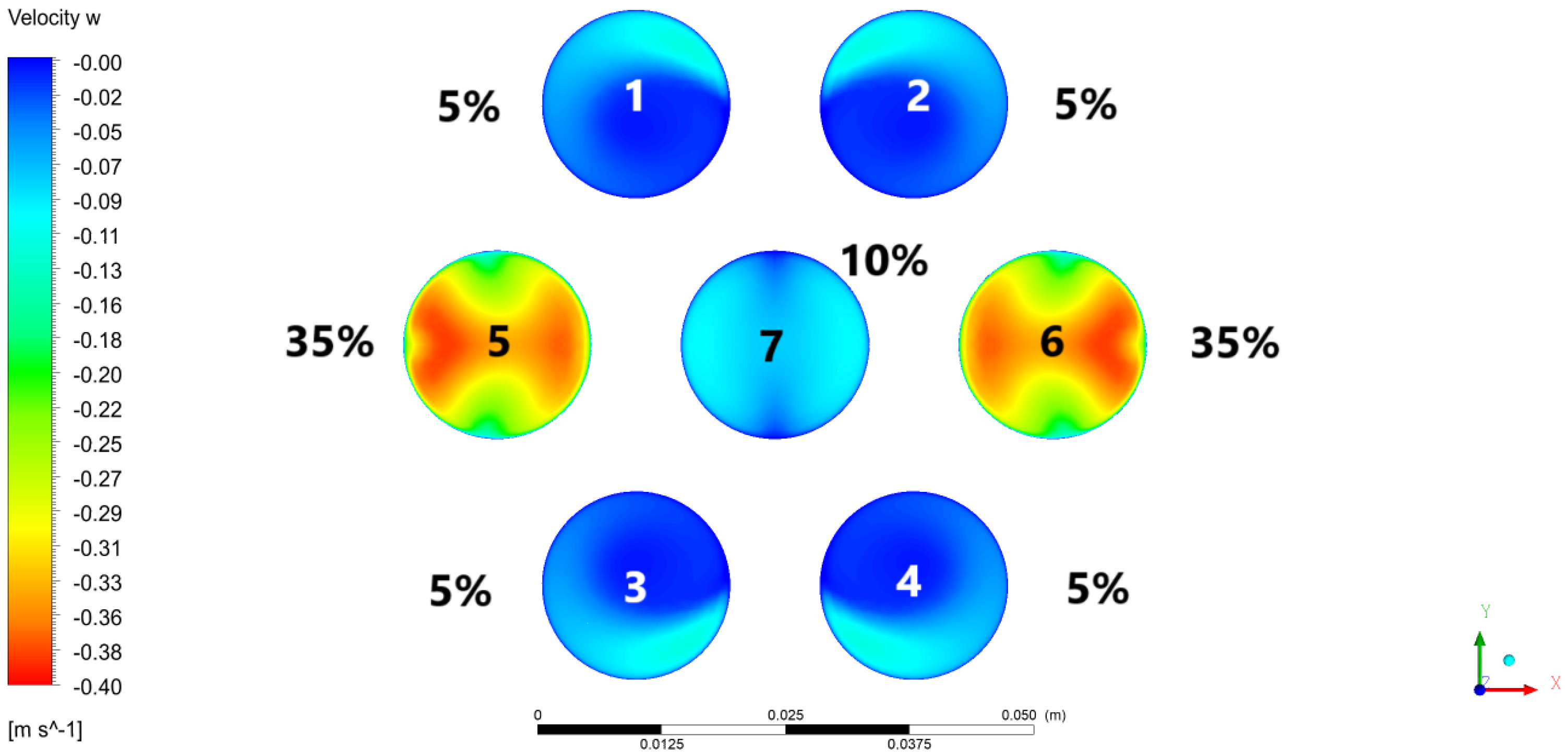
3.2. The Velocity Field in the Coolant Region

Next, an analysis of the mean velocity contours in the coolant region is reported. Despite the varying diameters of the coolant pipes in this zone, the mean velocity streamlines are primarily aligned in the axial z-direction (Figure 16). Only some flow perturbations are reported behind the fuel zone in the first quarter of the middle zone. This uniformity is expected since the coolant inlet flow direction is parallel to the pipes. This contrasts with the fuel flow, discussed in Section 3.1, where the presence of coolant pipes and sharp changes in flow direction in fuel distribution and collection zones created a more complex flow pattern.

Figure 17 presents the coolant velocities in the pipes within the C-1 plane (Figure 4), along with the percentage of the mass flow rate for each pipe related to the total mass flow rate of the coolant. In contrast to the fuel zone, the mass flow rates of the cooler region were almost the same for pipes of the same diameter. Interestingly, in the higher-diameter pipes, higher velocities were reported in the outer regions of the pipes.

As said, the coolant experiences some disturbances in the first quarter of the middle core zone. This effect is shown in Figure 16. These changes arise due to abrupt changes in the flow cross-sectional area and the presence of fuel pipes in the distribution zone, as shown in Figure 18. The flow is mostly driven upwards, visualised by negative w velocity components. However, some positive w velocity (reversed flow) is reported in the first zone of the middle core section due to the obstruction caused by the fuel pipes.

Not surprisingly, in the collection zone (Figure 19), the coolant exhibits the maximal values of the mean velocity comparable to those observed in the distribution zone (Figure 17). However, the velocity distribution within the larger-diameter pipes takes on a crescent shape in Figure 19, in contrast to the distribution zone, where higher velocities were concentrated in the outer region of the larger-diameter pipes (Figure 17). This indicates the flow circulation within the larger-diameter pipes in Figure 19.

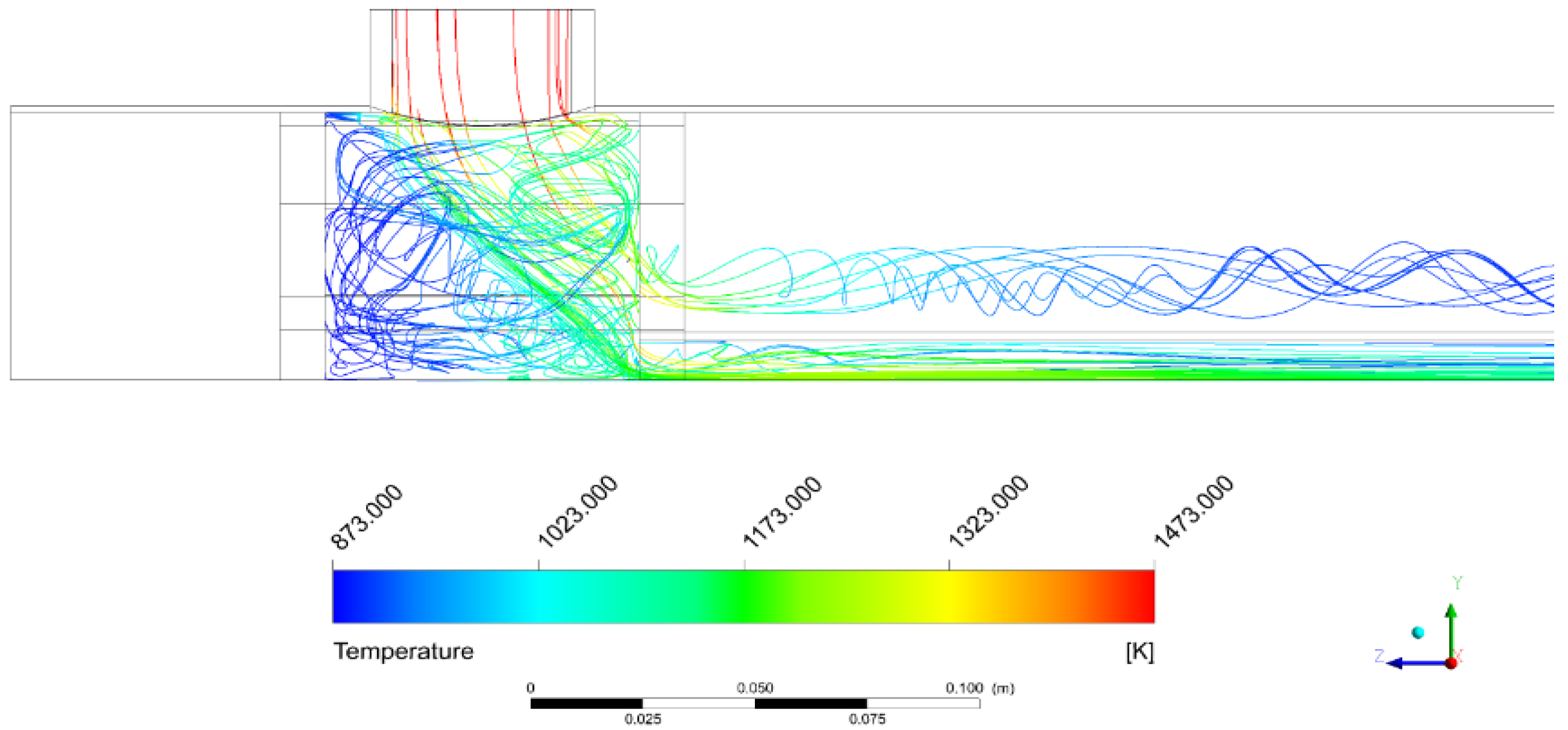
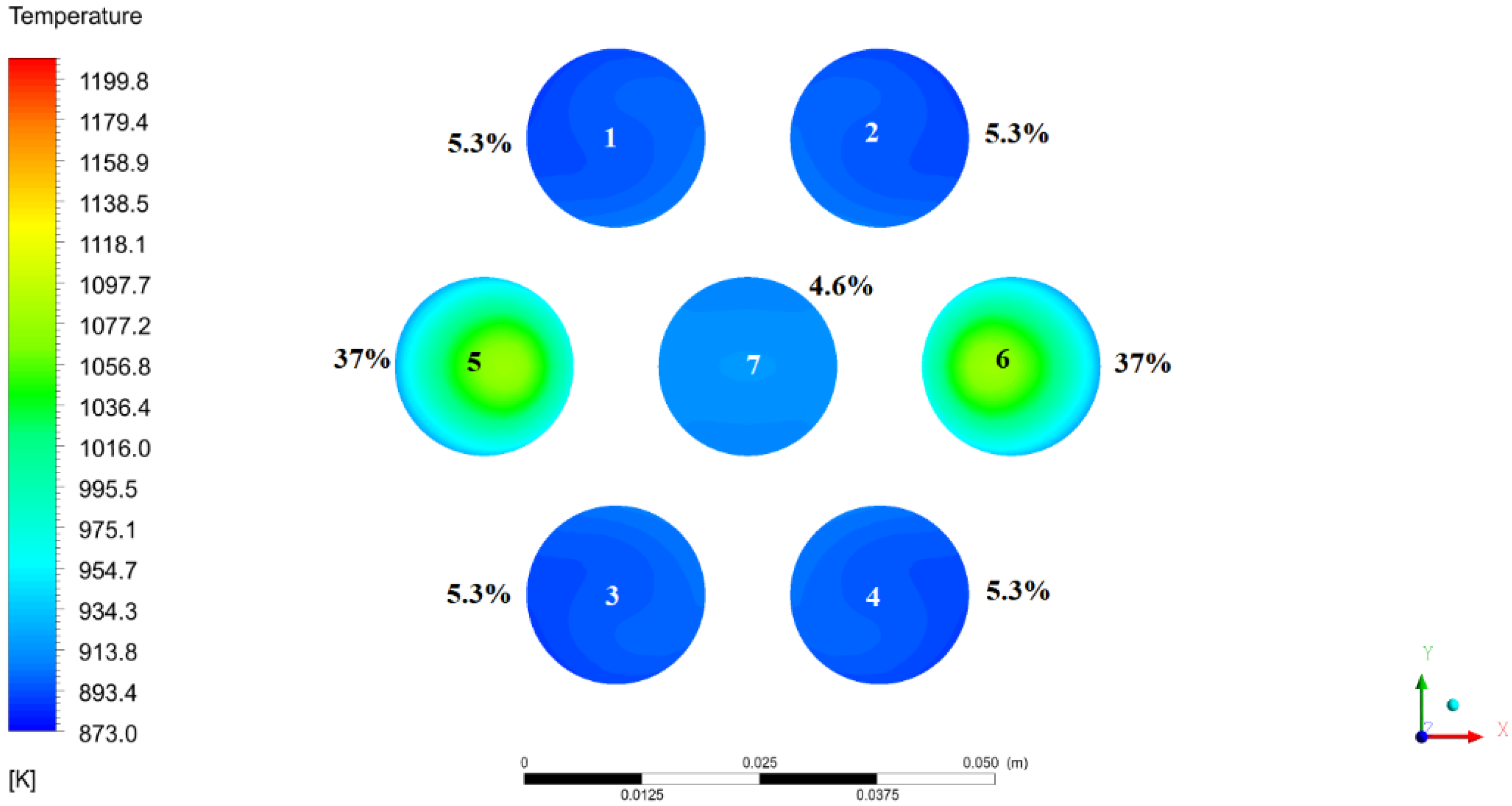
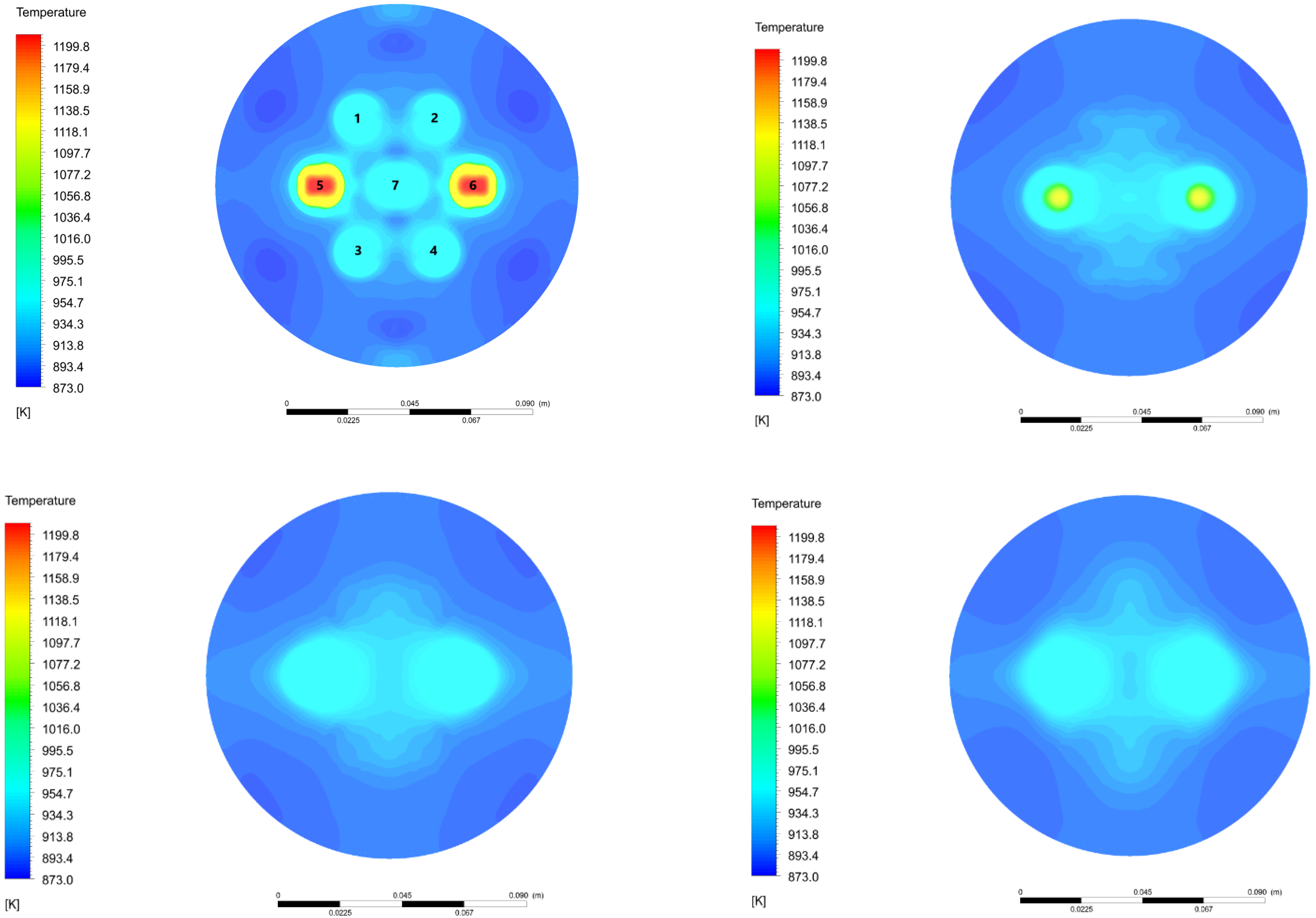
3.3. Heat Transfer in the Fuel Region

Heat transfer from fuel to coolant is the main target in any heat exchanger and has, in many cases, a complex mechanism [33]. In the fuel distribution zone, the incoming fuel flow is directed into the fuel pipes that are present in the core section of the MD (see Section 3.1). In this region, the fuel has its highest temperature while being in close contact with coolant pipes carrying coolant at its lowest temperature. This proximity results in significant heat transfer between the two mediums.

As shown in Figure 20, the flow within the distribution zone is characterised by two distinct regions with a notable temperature gradient. The high-temperature fuel enters from the MD inlet and redirects toward the fuel pipes due to its lower density and viscosity (buoyancy effect). It can be seen that an area of reduced temperature and velocity is established in the remaining part of the inlet section. We refer to the work by Todreas and Kazimi [34] for a discussion of the role of temperature-induced unsteadiness on flow and heat transfer in reactor systems.

In the collection zone (Figure 21), the fuel temperature is close to that of the coolant inlet, around 873 K. This indicates that most of the fuel’s heat has been effectively transferred to the coolant before reaching the collection zone.

Figure 22 shows the contour plots of temperature in the B-1 plane (Figure 3) of the fuel zone, together with the percentage of the heat transfer rate through the surfaces of the pipes. The temperature distribution is not uniform, similar to the velocity field discussed in earlier Figure 14. Surprisingly, 74% of heat flux occurs through the surfaces of only two pipes (#5 and #6 in Figure 22), leaving 26% to the remaining five pipes. Note that the strong flow and temperature non-uniformity were not expected at the beginning of this study, assuming the variable turbulent Prandtl number. One cannot expect a non-even distribution of the heat transfer rates on surfaces of pipes adopting some experimental correlations. So, this result justifies the selection of the CFD analysis of MD flow and heat transfer.

3.4. Heat Transfer in the Coolant Region

Figure 23 shows the contour plots of temperature on the coolant’s surfaces together with the fuel’s streamlines coloured by temperature. As the coolant enters the bottom side of the MD at 873 K, it absorbs a large amount of heat before leaving the distribution zone, primarily due to the presence of high-temperature fuel (1473 K) in this region. The figure shows the interaction between the fuel flow and cooler pipes and the rise in temperature on the surfaces of the cooler due to the high temperature of the impacting fuel. The coolant in the pipe directly facing the fuel inlet exhibits the highest temperature within the coolant domain.

In the region of the collection zone (Figure 24), the coolant temperature ranges from 886 to 920 K. The temperature increase is primarily a result of the heat absorbed in the earlier zones, specifically the distribution and middle core zones. The heat transfer occurring within this zone, however, is minimal.

3.5. Global Heat Transfer Characteristics

The heat transfer in the whole MD is greatly influenced by the temperature distribution and mass flow rates in each pipe. As demonstrated in Figure 14 and Figure 22, fuel pipes #5 and #6 exhibited the highest values of the mass flow rate and highest heat transfer rates through the surfaces of the pipes. Figure 25 presents the contour plots of temperature in four sections, B1–B4 (Figure 3). One can see that the highest temperature changes are reported next to pipes #5 and #6.

As discussed, the majority of heat transfer in the MD occurs within the initial quarter of the middle core zone (defined in Figure 1), followed by notable heat transfer in the distribution zone. In contrast, the collection zone demonstrates minimal heat transfer. To provide a more global picture of the heat transfer process, the heat transfer in each zone was calculated using the mass flow rate and the average temperature at both the inlet and outlet of the respective zones. For zones with multiple inlets, such as the pipes in the middle core zone, the average inlet conditions across the pipes were considered.

Table 5. Heat transfer in each zone in case of parallel flow.

Zone	Total Heat Transfer Rate Per Zone [kW]	Percentage of Heat Transfer [%]
Distribution zone	19	41.6
Middle Core zone	24.76	54.3
Collection zone	1.84	4.0
Total	45.6	100

provides a summary of the heat transfer in each zone, expressed in kilowatts (kW) and as a percentage of the total heat transfer occurring in analysed zones. The analysis shows that 41.6% and 54.3% of heat transfer is realised in the distribution and middle core regions, respectively. The collection zone has almost no role in the heat transfer process.

Next, the area-averaged temperature variations of the fuel and coolant were measured across six different planes: Inlets, B-1, B-2, B-3, B-4, and Outlets. Figure 26 illustrates the temperature distribution along these selected planes separately for fuel and cooler, highlighting the changes in temperature as the flow progresses through the system. The heat transfer distribution results in a sharp decline in fuel temperature during the first fifth of the heat exchange process within the MD core, where it drops from 1473 K to 990 K. This is followed by a substantial amount of heat transfer in the second fifth of the core, as reflected in the further reduction of fuel temperature from 990 K to 920 K.

The coolant temperature rises from 873 K to 895 K in the first fifth of the core (from the coolant inlet to plane B-1) but shows minimal further increase from B-1 to the coolant outlet.

The quantitative findings presented above highlight critical performance aspects, such as improved heat transfer and turbulence management, which are directly applicable to the optimisation of reactor designs. Building on these insights, this modelling approach offers significant potential for guiding advancements in DFR technology.

This modelling approach, incorporating the variable turbulent Prandtl number, provides a robust framework for guiding the design of future Dual Fluid Reactors (DFRs). By accurately capturing the thermal-hydraulic behaviour in critical regions, this methodology can aid in optimising coolant flow distribution to minimise hotspots, enhancing heat transfer efficiency in the reactor core. Furthermore, the insights into temperature gradients and turbulence effects can inform material selection and structural design, ensuring better resistance to thermal stresses. These advancements contribute to improving the safety and performance of next-generation DFRs while enabling scalability for industrial applications.

4. Conclusions

This study addressed critical gaps in the thermal-hydraulic modelling of Dual Fluid Reactors (DFRs) by implementing the Kays correlation to incorporate a variable turbulent Prandtl number into RANS simulations. This approach significantly improved the accuracy of heat transfer predictions for low-Prandtl-number liquids, overcoming the limitations of traditional models using a constant turbulent Prandtl number. The study applied this methodology to Reynolds numbers ranging from 15,000 to 250,000, with molecular Prandtl numbers of 0.025, enabling a detailed analysis of flow dynamics and heat transfer behaviour in the DFR mini demonstrator.

The results revealed uneven flow distributions within the fuel pipes, leading to variable temperature distribution across the reactor core. In some cases, hotspots exhibited very high-temperature gradients, with temperature changes of up to 200 °C within small areas. These findings highlight the importance of accurately modelling these localised variations, as such rapid temperature fluctuations can significantly affect reactor performance and safety. Furthermore, the mass flow rate in the fuel pipes was shown to vary significantly, with differences ranging from 5% to 35% between individual pipes, emphasising the need for precise modelling to capture the effects of flow imbalances on heat transfer and thermal efficiency.

The inclusion of a variable turbulent Prandtl number improved the prediction of thermal performance, yielding an enhancement in heat transfer accuracy over models with a constant Prandtl number. These insights provide a validated framework for addressing challenges in DFR thermal-hydraulic design and operational strategies. By identifying areas of potential structural stress and guiding the optimisation of flow dynamics, this study contributes to safer and more efficient next-generation nuclear systems. Future work will extend this modelling approach to more complex geometries and flow conditions, further enhancing its applicability to advanced reactor technologies.

References

1. Muellner, N.; Arnold, N.; Gufler, K.; Kromp, W.; Renneberg, W.; Liebert, W. Nuclear Energy—The Solution to Climate Change? Energy Policy 2021, 155, 112363. [Google Scholar] [CrossRef]
2. Nuclear Energy Agency (NEA). Technology Roadmap Update for Generation IV Nuclear Energy Systems; Technical Report; U.S. DOE Nuclear Energy Research Advisory Committee and the Generation IV International Forum: Washington, DC, USA, 2014. [Google Scholar]
3. Wang, X.; Macian-Juan, R. Comparative Study of Basic Reactor Physics of the DFR Concept Using U-Pu and TRU Fuel Salts. In Proceedings of the International Conference on Nuclear Engineering, Shanghai, China, 2 July 2017; ASME International: New York, NY, USA, 2017. [Google Scholar]
4. Huke, A.; Ruprecht, G.; Weißbach, D.; Czerski, K.; Gottlieb, S.; Hussein, A.; Herrmann, F. Dual-Fluid Reactor. In Molten Salt Reactors and Thorium Energy; Elsevier: Amsterdam, The Netherlands, 2017; pp. 619–633. ISBN 9780081012437. [Google Scholar]
5. Wang, X.M. Analysis and Evaluation of the Dual Fluid Reactor Concept. Ph.D. Thesis, Technischen Universität München, Munich, Germany, 2017. [Google Scholar]
6. Singh, O.P. Nuclear Reactors of the Future. In Physics of Nuclear Reactors, 1st ed.; Elsevier: Amsterdam, The Netherlands, 2021. [Google Scholar]
7. Roelofs, F. Liquid Metal Thermal Hydraulics: State-of-the-Art and Future Perspectives. Nucl. Eng. Des. 2020, 362, 110590. [Google Scholar] [CrossRef]
8. Grötzbach, G. Challenges in Low-Prandtl Number Heat Transfer Simulation and Modelling. Nucl. Eng. Des. 2013, 264, 41–55. [Google Scholar] [CrossRef]
9. Wang, X.; Liu, C.; Macian-Juan, R.; Wang, X.; Liu, C.; Macian-Juan, R. Preliminary Hydraulic Analysis of the Distribution Zone in the Dual Fluid Reactor Concept. In Proceedings of the International Topical Meeting on Nuclear Reactor Thermal Hydraulics, Xi’an, China, 3–8 September 2017. [Google Scholar]
10. Toki, T.; Teramoto, S.; Okamoto, K. Velocity and Temperature Profiles in Turbulent Channel Flow at Supercritical Pressure. J. Propuls. Power 2020, 36, 3–13. [Google Scholar] [CrossRef]
11. Elgendy, H.; Czerski, K. Numerical Study of Flow and Heat Transfer Characteristics in a Simplified Dual Fluid Reactor. Energies 2023, 16, 4989. [Google Scholar] [CrossRef]
12. Shams, A.; De Santis, D.; Padee, A.; Wasiuk, P.; Jarosiewicz, T.; Kwiatkowski, T.; Potempski, S. High-Performance Computing for Nuclear Reactor Design and Safety Applications. Nucl. Technol. 2020, 206, 283–295. [Google Scholar] [CrossRef]
13. Kays, W.-M. Turbulent Prandtl Number. Where Are We? ASME J. Heat Transf. 1994, 116, 284–295. [Google Scholar] [CrossRef]
14. Weigand, B.; Ferguson, J.R.; Crawford, M.E. An Extended Kays and Crawford Turbulent Prandtl Number Model. Int. J. Heat Mass Transf. 1997, 40, 4191–4196. [Google Scholar] [CrossRef]
15. Huang, J.; Nicholson, G.L.; Duan, L.; Choudhari, M.M.; Bowersox, R.D. Simulation and Modeling of Cold-Wall Hypersonic Turbulent Boundary Layers on Flat Plate. In Proceedings of the AIAA Scitech 2020 Forum, Orlando, FL, USA, 6–10 January 2020; American Institute of Aeronautics and Astronautics: Reston, VA, USA, 2020. [Google Scholar]
16. Shams, A.; De Santis, A. Towards the Accurate Prediction of the Turbulent Flow and Heat Transfer in Low-Prandtl Fluids. Int. J. Heat Mass Transf. 2019, 130, 290–303. [Google Scholar] [CrossRef]
17. De Santis, D.; De Santis, A.; Shams, A.; Kwiatkowski, T. The Influence of Low Prandtl Numbers on the Turbulent Mixed Convection in an Horizontal Channel Flow: DNS and Assessment of RANS Turbulence Models. Int. J. Heat Mass Transf. 2018, 127, 345–358. [Google Scholar] [CrossRef]
18. Liu, C.; Li, X.; Luo, R.; Macian-Juan, R. Thermal Hydraulics Analysis of the Distribution Zone in Small Modular Dual Fluid Reactor. Metals 2020, 10, 1065. [Google Scholar] [CrossRef]
19. Huke, A.; Ruprecht, G.; Weißbach, D.; Gottlieb, S.; Hussein, A.; Czerski, K. The Dual Fluid Reactor—A Novel Concept for a Fast Nuclear Reactor of High Efficiency. Ann. Nucl. Energy 2015, 80, 225–235. [Google Scholar] [CrossRef]
20. Al-Habahbeh, O.M.; Al-Saqqa, M.; Safi, M.; Abo Khater, T. Review of Magnetohydrodynamic Pump Applications. Alex. Eng. J. 2016, 55, 1347–1358. [Google Scholar] [CrossRef]
21. Nowak, M.; Spirzewski, M.; Czerski, K. Optimization of the DC Magnetohydrodynamic Pump for the Dual Fluid Reactor. Ann. Nucl. Energy 2022, 174, 109142. [Google Scholar] [CrossRef]
22. Smith, C.F.; Halsey, W.G.; Brown, N.W.; Sienicki, J.J.; Moisseytsev, A.; Wade, D.C. SSTAR: The US Lead-Cooled Fast Reactor. J. Nucl. Mater. 2008, 376, 255–259. [Google Scholar] [CrossRef]
23. Smith, C.F.; Cinotti, L. Lead-Cooled Fast Reactors. In Handbook of Generation IV Nuclear Reactors, 2nd ed.; Pioro, I.L., Ed.; Woodhead Publishing: Cambridge, UK, 2022. [Google Scholar]
24. Smith, C. Lead-Cooled Fast Reactor (LFR) Design: Safety, Neutronics, Thermal Hydraulics, Structural Mechanics, Fuel, Core, and Plant Design; U.S. Department of Energy, Office of Scientific and Technical Information: Oak Ridge, TN, USA, 2010.
25. Kawamura, H.; Ohsaka, K.; Abe, H.; Yamamoto, K. DNS of Turbulent Heat Transfer in Channel Flow with Low to Medium-High Prandtl Number Fluid. Int. J. Heat Fluid Flow 1998, 19, 482–491. [Google Scholar] [CrossRef]
26. Menter, F.R. Two-Equation Eddy-Viscosity Turbulence Models for Engineering Applications. AIAA J. 1994, 32, 1598–1605. [Google Scholar] [CrossRef]
27. Hanjalić, K.; Launder, B. Modelling Turbulence in Engineering and the Environment; Cambridge University Press: Cambridge, UK, 2022; ISBN 9781108875400. [Google Scholar]
28. Duponcheel, M.; Bricteux, L.; Manconi, M.; Winckelmans, G.; Bartosiewicz, Y. Assessment of RANS and Improved Near-Wall Modeling for Forced Convection at Low Prandtl Numbers Based on LES up to ReT = 2000. Int. J. Heat Mass Transf. 2014, 75, 470–482. [Google Scholar] [CrossRef]
29. Nilsson, O.; Mehling, H.; Horn, R.; Fricke, J.; Hofmann, R.; Müller, S.; Eckstein, R.; Hofmann, D. Determination of the Thermal Diffusivity and Conductivity of Monocrystalline Silicon Carbide (300–2300 K). High Temp. High Press. 1997, 29, 73–79. [Google Scholar] [CrossRef]
30. Nuclear Energy Agency. Handbook on Lead-Bismuth Eutectic Alloy and Lead Properties, Materials Compatibility, Thermal-Hydraulics and Technologies; Organisation for Economic Co-Operation and Development: Paris, France, 2015. [Google Scholar]
31. ANSYS, Inc. ANSYS Fluent Theory Guide; ANSYS, Inc.: Canonsburg, PA, USA, 2021. [Google Scholar]
32. Ferziger, J.H. High-Order Methods for Computational Physics, 3rd ed.; Springer: Berlin, Germany, 2002. [Google Scholar]
33. Incropera, F.P.; Dewitt, D.P.; Bergman, T.L.; Lavine, A.S. Fundamentals of Heat and Mass Transfer, 6th ed.; John Wiley & Sons: Hoboken, NJ, USA, 2006. [Google Scholar]
34. Todreas, N.E.; Kazimi, M.S. Nuclear Systems: Thermal Hydraulic Fundamentals, 2nd ed.; CRC Press: Boca Raton, FL, USA, 2011; Volume 1. [Google Scholar]
Figure 1. MD core zones and elements: 1 is the distribution zone, 2 is the middle core zone, and 3 is the collection zone.
Energies 18 00396 g001
Figure 2. Longitudinal plane A.
Energies 18 00396 g002
Figure 3. In-core Transverse planes B1–B4.
Energies 18 00396 g003
Figure 4. Transverse Inlet/Outlet planes C1, C2.
Energies 18 00396 g004
Figure 5. Distribution zone (quarterly sliced): blue represents the coolant, and red represents the fuel.
Energies 18 00396 g005
Figure 6. Temperature profiles normalised by friction temperature for simulation of the fully developed channel flow with Pr = 0.025. LES ( R e τ = 2000 ), Kays (variable Prt) and constant value of the turbulent Prandtl number (Prt = 0.85).
Energies 18 00396 g006
Figure 7. Details of computational mesh in distribution/collection zones: y–z plane (top), x–z plane (bottom).
Energies 18 00396 g007
Figure 8. Three planes in the distribution zone.
Energies 18 00396 g008
Figure 9. The side view in the distribution zone shows fuel pipes (orange), coolant pipes (blue) and fuel entrance direction.
Energies 18 00396 g009
Figure 10. Contour plots of velocity magnitude [m/s] in the distribution zone for plans (AC) obtained with variable (left) and constant (right) values of the turbulent Prandtl numbers.
Energies 18 00396 g010
Figure 11. Contour plots of static temperature [K] in the distribution zone for plans (AC) obtained with variable (left) and constant (right) values of the turbulent Prandtl numbers.
Energies 18 00396 g011
Figure 12. Contour plot of velocity magnitude [m/s] in C-1 plane (distribution zone).
Energies 18 00396 g012
Figure 13. Flow streamlines coloured by velocity magnitude in the distribution zone.
Energies 18 00396 g013
Figure 14. Contour plot of w velocity component (z-direction) in B-1 plane with the percentage of the fuel mass flow rate in each pipe. An inverse rainbow colour code is used due to the negative z velocity component.
Energies 18 00396 g014
Figure 15. Streamlines coloured by velocity magnitude in the collection zones.
Energies 18 00396 g015
Figure 16. Streamlines coloured by velocity magnitude in the distribution zone of the coolant.
Energies 18 00396 g016
Figure 17. Contour plot of coolant in C-1 plane with percentage of the mass flow in each pipe.
Energies 18 00396 g017
Figure 18. Contour plots of w velocity component in the coolant domain. An inverse rainbow colour code is used to denote the velocity component opposite to the z-direction.
Energies 18 00396 g018
Figure 19. Contour plots of velocity magnitude in the C-2 plane (Figure 4) in the coolant region (collection zone).
Energies 18 00396 g019
Figure 20. Flow streamlines of fuel coloured by static temperature in the distribution zone.
Energies 18 00396 g020
Figure 21. Flow streamlines of fuel in the collection zone with temperature-coded colour.
Energies 18 00396 g021
Figure 22. Contour plots of temperature in the B-1 plane in the fuel zone with heat transfer percentage in each pipe along the middle core zone.
Energies 18 00396 g022
Figure 23. Contour plot of coolant temperature on surfaces of MD in the distribution zone together with temperature-colour-coded fuel streamlines.
Energies 18 00396 g023
Figure 24. Flow streamlines coloured by static temperature in the collection zone of MD.
Energies 18 00396 g024
Figure 25. Fuel-pipe-coolant temperature contours in the middle core zone in planes B-1 to B-4 (From top-left, through top-right, bottom-left to bottom-right).
Energies 18 00396 g025
Figure 26. Area averaged temperature profile in case of parallel flow.
Energies 18 00396 g026