Optimization of Well Locations and Trajectories: Comparing Sub-Vertical, Sub-Horizontal and Multi-Lateral Well Concepts for Marginal Geothermal Reservoir in The Netherlands

Abstract

Scaling up the direct use of geothermal heat in urban areas comes with the challenge of enabling the development of projects in geological settings where geothermal reservoir flow properties may be poor, resulting in low well flow performance. Cost-effective field development strategies and well designs tailored to such reservoirs can ensure the deliverability of geothermal energy in economic terms. This study presents a framework based on computer-assisted optimization to support practitioners in selecting the most suitable well concept for the exploitation of such marginal geothermal reservoirs. The proposed methodology is illustrated in a real-life case study of a geothermal development prospect in an urban area in The Netherlands, where the performance of sub-vertical, sub-horizontal and multi-lateral wells is compared. The obtained results indicate that the techno-economic performance of the geothermal doublet can be significantly improved by optimization, for all considered well concepts, and that, despite the importance of selecting the well concept, well location is still the main determinant of an effective field development strategy. The sub-horizontal and multi-lateral well concepts appear to be the most suitable for the target case study, outperforming the sub-vertical doublets, with a higher expected net present value and a lower economic variability risk for the multi-lateral solution.

1. Introduction

The success of the energy transition in our society heavily depends on our capacity to improve the cost-effectiveness of the technologies involved. Renewable heat provision can be strongly facilitated by subsurface resources [1], both as a source of geothermal energy and for seasonal storage purposes [2]. Scaling up the direct use of geothermal heat requires developing resources close to existing areas of demand or available heat transport infrastructure. From this perspective, a particular technological challenge refers to the ability of enabling the techno-economic feasibility of geothermal developments in areas where the subsurface properties might be sub-optimal for geothermal energy extraction [3], typically with a mismatch between locations of heat demand and those with the best-quality geothermal resources. Figure 1 highlights this notion for The Netherlands, a densely populated country in Northern Europe with over 25 cities, with a population of over 100,000, with significant urban heat demand in the order of 800 PJ/year, and an associated wide areal distribution of district heat networks. These could potentially be sourced by geothermal energy. However, extensive analysis of geothermal resource potential in the past decade, as supported by a wealth of subsurface data from past hydrocarbon exploration and production ([4,5,6]; https://thermogis.nl, accessed on 20 September 2024), has demonstrated that geothermal resource quality is spatially diverse, and as a consequence, marginal or poor reservoir quality hinders the development of geothermal district heating in many cities.

In this context, the choice of fit-for-purpose field development strategies and, more importantly, effective well designs play a pivotal role to ensure the provision of geothermal energy in economic terms. In addition to being geared to poor reservoir performance, well designs should take into account the limited availability of surface locations, which will raise further challenges for selecting the most suitable well designs, honoring both constraints on surface locations for well drilling platforms and technically feasible and cost-effective well engineering options.

Several reservoir engineering studies have focused on the assessment and optimization of well placement and well trajectory configurations, mostly in the oil and gas sector [7,8,9], but with an increasing number of applications in other geo-energy settings, like the geothermal energy domain [10,11,12,13,14]. The optimization of well locations and trajectories are typically guided by techno-economic performance indicators to compare various configurations for the identification of the most cost-effective solutions. While this kind of optimization usually aims to maximize the cost-efficiency of geothermal energy production, in some cases it is also applied as a means to ensure the safety and viability of the geothermal project by minimizing undesired effects, such as induced seismicity or fault reactivation [15,16]. In order to employ numerical optimization, the problem also must be formulated mathematically in terms of parametrization of optimization variables to represent possibly complex well trajectories [9]. Another aspect to be taken into account is the uncertainty associated with the subsurface flow properties, which have a direct impact on the expected effectiveness of selected well locations and designs [12,14,17,18].

Most of the reported studies narrow down the scope of optimization to a given type of well, e.g., vertical wells and horizontal wells. And few of those have investigated the use of optimization in more complex well designs, e.g., multi-lateral wells. In this work, we present a more comprehensive well design optimization study where we employ computer-assisted optimization (based on the stochastic gradient method) to three types of wells to provide geothermal practitioners with the quantitative and comparative insights needed to support their choice of well concept for a real-life target case study.

This paper is structured as follows. In Section 2, we introduce the optimization methodology tailored to complex well designs for marginal reservoirs, including a brief theoretical background of the numerical optimization techniques applied and a description of the computational workflow with the extensions to support the optimization of multi-lateral wells. In Section 3, we delineate the case study reservoir parameters in terms of the concept select context, modeling assumptions, and boundary conditions for the optimization experiments. In Section 4, we analyze the results of the optimization study and contrast the performance of the various well concepts. Finally, in Section 5, we summarize the main findings of the work with concluding remarks and directions for future work.

2. Methodology

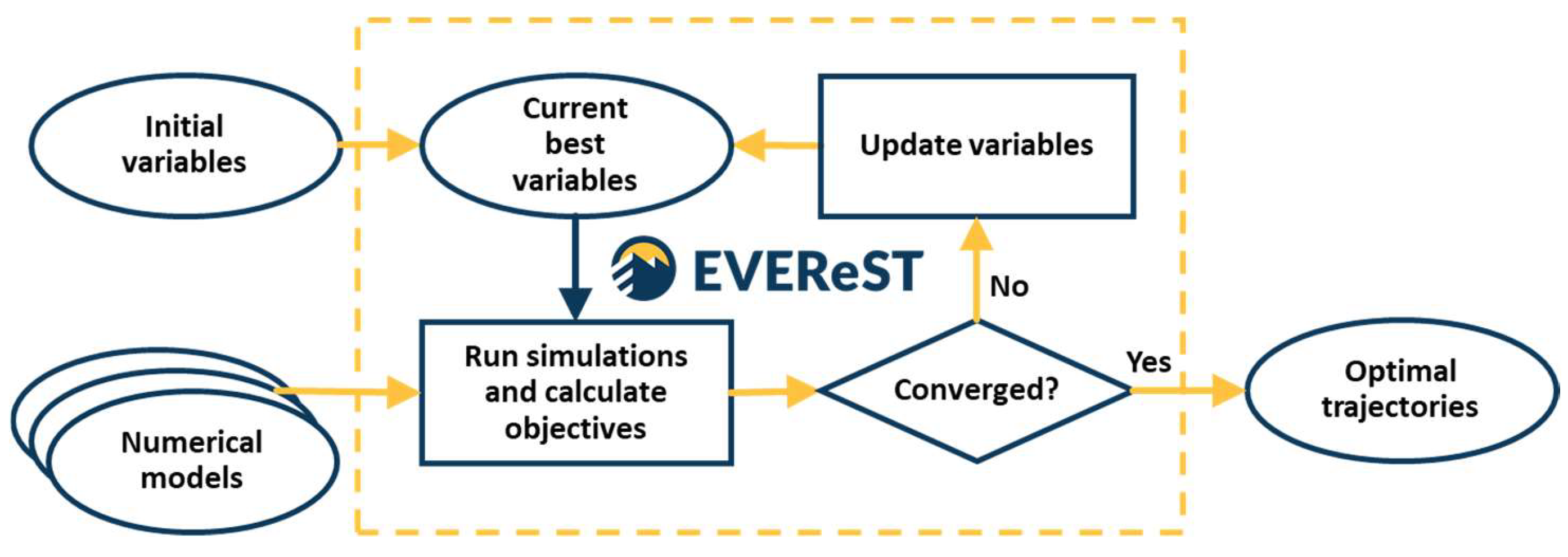
2.1. Optimization Approach

The aim is to provide project developers with an objective insight into the most suitable well concept to develop a geothermal reservoir. To this end, we have devised a methodology to quantitatively analyze and rank the potential techno-economic performance of various well concepts. The proposed methodology is supported by computer-assisted optimization, which allows for a broader exploration of possible well configurations and for accounting for the impact of geological uncertainty, as well as surface constraints for engineering. The idea is to optimize doublet configurations (i.e., well trajectories and locations) for each well concept considered and identify the best performing optimized configuration across the different concepts. The rationale is that the fairest and most meaningful way of contrasting well concepts to select or discard them is by comparing optimized configurations—contrasting concepts based on arbitrarily (and most likely sub-optimally) chosen configurations could lead to wrong decisions.

In order to achieve the abovementioned goal, the work carried out consists of the following steps.

• Generate an ensemble of base case (dynamic) simulation models of the geothermal reservoir to represent the inherent uncertainty associated with geological parameters:

  a.

  Construct a 3D static geological model accounting for uncertain reservoir flow properties;

  b.

  Assemble an ensemble of reservoir model realizations following prescribed production constraints.

• Define the well trajectory optimization problem:

  a.

  Specify the optimization variables (here, well trajectories and locations) and their optimization constraints;

  b.

  Set economic parameters of techno-economic objective function.

• Perform well trajectory optimization experiments for different well concepts:

  a.

  Experiment 1: sub-vertical wells;

  b.

  Experiment 2: sub-horizontal wells;

  c.

  Experiment 3: multi-lateral wells (with 3 branches).

• Analyze and compare the results of the optimization experiments performed in (3) to derive case-specific insights and recommendations for well concept selection.

Next, we describe the optimization framework employed in this work by briefly outlining the numerical optimization techniques and iterative procedure adopted and by presenting the workflow for optimizing well trajectories.

2.2. Numerical Optimization Framework

Model-based optimization methods can be grouped into two types: derivative-free and derivative (gradient)-based approaches. Derivative-based methods are the most computationally efficient for problems with expensive objective functions, but they require access to the analytical derivatives from the numerical simulator. As a result, these methods have limited practical applicability due to the need to alter the simulator code. To circumvent this, recent studies have increasingly focused on the use of stochastic gradients [9,19,20,21,22,23,24,25,26], which are easy to implement and provide flexibility, since the simulator can be used as a black box. This allows for any type of objective function (derived from outputs of a simulation model) and optimization variables to be incorporated with minimal effort. Stochastic gradient methods are also computationally attractive for robust optimization applications, where uncertainty is accounted for throughout the entire optimization procedure. Stochastic gradients can be regarded as a sort of hybridization of derivative-free and traditional gradient-based techniques, benefiting from the strengths of both classes of methods whilst addressing their drawbacks.

In this work, we employ the Stochastic Simplex Approximate Gradient (StoSAG) technique [19], an approach for robust optimization supported by an ensemble of model scenarios. To calculate the approximate gradient of the objective function with respect to the optimization variables (or controls), a set of statistical perturbations around the initial controls is generated by simultaneously sampling all the control variables based on a Gaussian distribution centered in the original control. The perturbed control points are then evaluated in terms of their objective function (by running reservoir simulations and calculating techno-economic indicators). Next, a linear regression step is performed on this collection of perturbed points (i.e., control and objective values) to estimate an approximate gradient. This stochastic gradient supplies a direction for updating the controls towards solutions with improved values for the objective function in the iterative optimization procedure (Figure 2). The StoSAG technique is available within our open-source optimization framework, EVEREST™ (www.everest.tools; https://www.github.com/equinor/everest, accessed on 16 December 2024).

When uncertainty is represented through an ensemble of model realizations, it is possible to pair each model realization with a single control perturbation [19], inspired by the approach followed by [27]. This significantly reduces the number of (typically expensive) function evaluations required to estimate the gradient and, in turn, the computational cost of the optimization procedure in large-scale problems. In this paper, the focus is on the application of the EVEREST framework using the StoSAG method for well trajectory optimization in a real-life case with the purpose of comparing and screening well concepts. In light of this, the StoSAG method is only briefly described in its essence here—for more details, refer to [19].

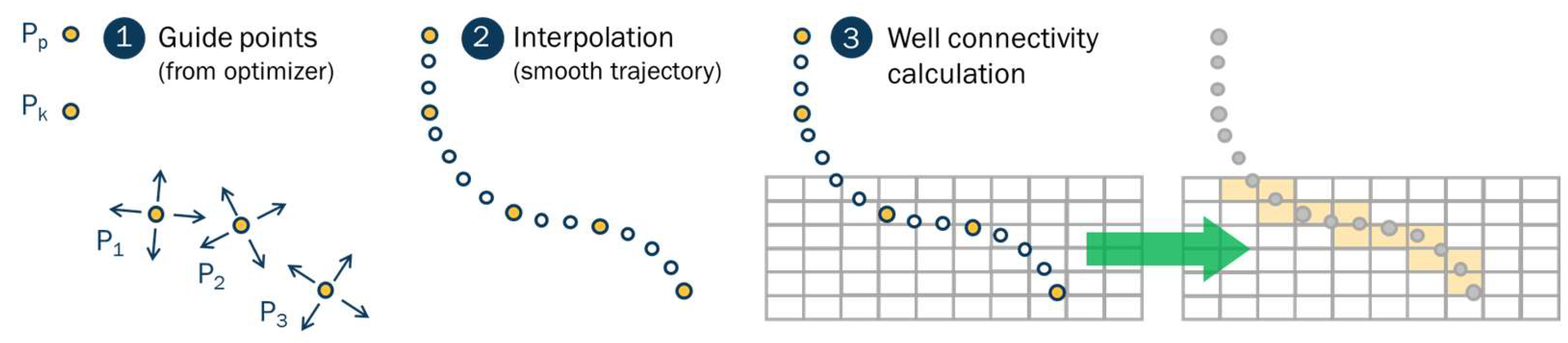
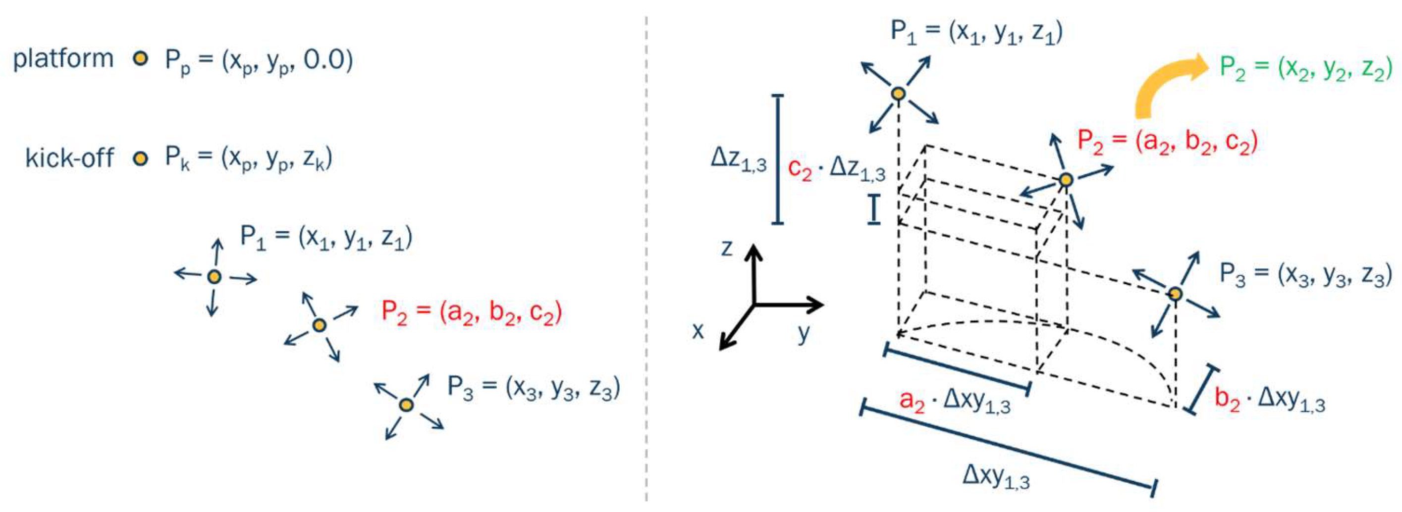
2.3. Parametrization of Well Trajectories

An important part of the workflow based on computer-assisted optimization consists of mathematically representing the variables to be optimized. In the following sub-sections, we describe the approach adopted within the EVEREST optimization framework to parametrize complex well trajectories with a reduced number of control variables.

2.3.1. Standard Wells

Standard wells consist of wells with a single branch (or leg). Trajectories of standard wells may range from perfectly vertical to fully straight horizontal wells within the reservoir section, including any type of curvilinear deviated configurations in between. In order to realistically represent various types of standard well trajectories, we adopt a general parametrization proposed by [9], based on prescribing the coordinates of a small number of target points. This is desirable because it simplifies the number of variables to be handled by the optimizer, which, in general, contributes to improving the optimization performance. The target points control the overall span of the trajectories, and the minimum curvature method [28] (here accomplished with functionality available in the open-source post-processing tool ResInsight: https://resinsight.org/, accessed on 13 October 2024) is used to reconstruct smooth drillable well paths connecting the target points while honoring the imposed constraints on the maximum allowed dogleg severity. Each well trajectory is parametrized by a platform location (x, y) (P_p in Figure 3), a kick-off depth (z) (P_k in Figure 3) and 3 reservoir target points (x, y, z) (P₁, P₂ and P₃ in Figure 3). See all the points shown as yellow dots in Figure 3. This means that each well is characterized by a total of 12 variables to describe its 5 target points: P_p, P_k, P₁, P₂ and P₃. The smooth well paths are characterized by a larger amount of interpolated points (white points in Figure 3), describing the geometry of the well via high-resolution piece-wise linear segments, as commonly specified by drilling engineers in terms of well deviation data.

The calculation of the well connection factors is a key step in the well trajectory optimization workflow, as these values determine the inflow between the well and the reservoir. This requires access to the well path information (x, y, z coordinates of points sampling three-dimensional drilling path of the wells) and grid information of the reservoir simulation model to determine (1) the grid blocks intercepted by the well trajectories and (2) the well connection factors at those grid blocks. Even though the workflow is equipped with capabilities to filter out grid cell connections based on grid properties (e.g., depth, permeability, temperature), this was not the case in this work—thus, in this study, wells are assumed to be perforated and connected to all grid cells intercepted by their trajectories. Figure 4 illustrates the geometric parametrization in more detail. In order to constrain the monotonicity of the well trajectories, the coordinates of P₁ and P₃ are parametrized independently, while the coordinates of P₂ are defined through projection values (a₂, b₂, c₂) as a function of P₁ and P₃. a₂ is the scaled projection parameter controlling the horizontal deviation between P1 and P3: when a₂ → 0, P₂ is positioned closer to P₁; when a₂ → 1, it is closer to P₃. b₂ is the scaled deflection parameter controlling the lateral bending of the trajectory between P₁ and P₃: when b₂ → 0, the trajectory is a straight line; otherwise, the trajectory is bended (the sign b₂ indicates the bending side). c₂ is the scaled projection parameter controlling the vertical elevation of P₂ with respect to P₁ and P₃: when c₂ → 0, P₂ is positioned closer to P₃; when c₂ → 1, it is closer to P₁. a₂ and c₂ combined determine the vertical bending of the trajectory between P₁ and P₃: in a situation where P₃ is deeper than P₁, the trajectory will be concave upward for low values of a₂ and c₂, and concave downward for high values of a₂ and c₂. Based on the x, y and z coordinates of P₁ and P₃ and the projection values a₂, b₂ and c₂, the x, y and z coordinates of P₂ are calculated and the workflow can then proceed to the interpolation step.

We note that this mathematical parametrization of well trajectories is completely grid-independent. None of the target points have their coordinates defined relatively to the geometry of the grid of the reservoir model (e.g., top/bottom of reservoir formation). As a result, well trajectories have the freedom to move out of the reservoir model during optimization, allowing the optimizer to determine the optimal well–reservoir contact, and, in case of multiple wells, to identify potentially unnecessary wells that should not be drilled.

2.3.2. Multi-Lateral Wells

In order to handle the optimization of multi-lateral wells, the workflow for standard wells described above needs to be extended. The steps of the workflow remain essentially the same as depicted in Figure 3, but the mathematical parametrization has to be expanded with additional variables, and the interpolation and connectivity calculations must be performed for all branches or legs of the multi-lateral well.

The expanded parametrization for multi-lateral wells follows the same approach of the parametrization of the standard wells. First, the main branch of the multi-lateral is parametrized as a standard well (i.e., with the 5 target points from Figure 4). Next, one by one, the additional branches are parametrized by 3 target points each, equivalent to P₁, P₂ and P₃ from the standard well parametrization. However, the first target point of each branch (i.e., the one analogous to P₁) determines the branching out point and is described by a single variable controlling its position in terms of measured depth (or along-hole depth) along the trajectory of the main branch, from which it is possible to calculate its x, y and z coordinates. The other two points follow the exact same logic of P₂ and P₃ in the standard well parametrization. In this work, the number of multi-lateral legs is fixed to 3 (i.e., 1 main branch, plus 2 additional legs). Here, it is also assumed that both additional legs branch out at the same point along the main branch. Figure 5 illustrates the expanded parametrization. In this case, each multi-lateral well with 3 legs is described by a total of 10 target points and 25 variables: (i) 5 points for the main branch (P_p, P_k, P₁, P₂, P₃) with 12 variables, (ii) 3 points for the first leg (P₄, P₅, P₆) with 7 new variables (1 × MD for P4 and 2 × (x, y, z) for P₅ and P₆) and (iii) 3 points for the second leg (P₄, P₇, P₈) with 6 new variables (2 × (x, y, z) for P₇ and P₈–P₄ is already characterized).

In order to ensure the feasibility of the multi-lateral leg drilling in terms of the maximum allowed curvature (i.e., dogleg severity), the interpolation step is applied, assuming each leg, to form a single continuous trajectory from the surface location to the last target point, i.e., P_p, P_k, P₄, P₅, P₆ for the first leg, and P_p, P_k, P₄, P₇, P₈ for the second leg. Note that no explicit geometric constraints are imposed to avoid collision or cross-over between the individual legs, although such geometric constraints could be defined. The cost for well length included in the objective function ensures implicitly that the legs increase contact with the reservoir, which is not the case if they cross.

3. Case Study

3.1. Surface Drilling Location

This study concerns a geothermal doublet to serve the future heat demand of an urban area. Because it is situated in a relatively densely occupied area, there is a limited number of lots potentially available for the deployment of a drilling wellsite in the vicinity of the municipality. Combined with the drilling risks associated with long wellbores and large outsteps, this restriction in available surface locations poses a technical challenge to the placement of wells to reach subsurface targets in the geothermal reservoir.

A candidate wellsite location for this geothermal project was identified prior to this study. That surface drilling location (P_p as defined within our adopted parametrization described in Section 2.3) is kept fixed throughout our well trajectory optimization. The other target points characterizing the well trajectory remain as degrees of freedom available for optimization. As a starting point for the optimization, the wells penetrate the reservoir area just below the designated surface drilling location. Throughout the techno-economic optimization exercise, longer wells are penalized by higher costs, and the total outstep of the wells is monitored to ensure it remains within the acceptable range (approx. 3000 m, as defined prior to this study based on typically feasible well geometry assumptions for a well reaching the depth of the target reservoir, ~2500 m). In the case that total well lengths and outsteps exceed the values accepted as feasible, another surface location is needed. The maximum allowed dogleg severity value in this work was 4°/100 ft.

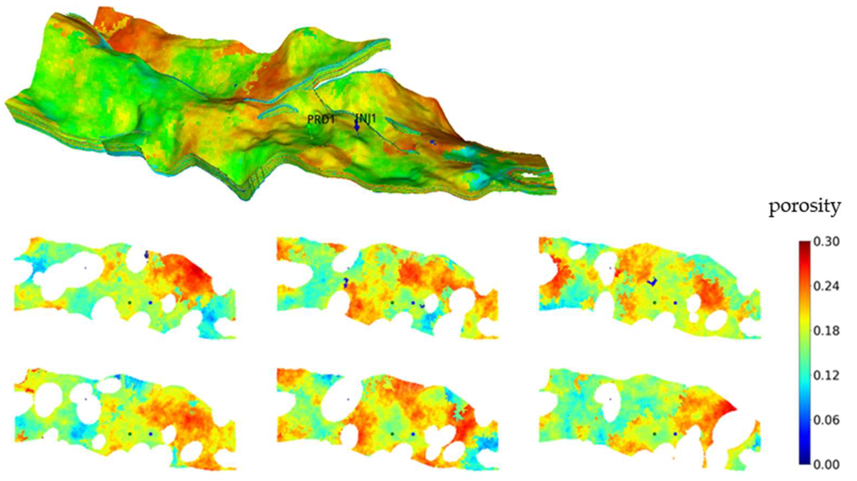
3.2. Geological Characterization

In order to provide the information required to assess the viability of well concepts in the area of interest, a conventional subsurface characterization study was performed by combining insights from structural, geological, petrophysical and fluid analysis to understand the expected subsurface properties and uncertainties associated with the reservoir flow performance.

The Rotliegend reservoir in the area of interest is usually composed of conglomerates at the base, with a sequence of dune sands decreasing in grain size upwards, on the top. Some ponded lake sediments are also identified. The reservoir quality (permeability) of the sands is generally average to good; however, local cementation resulting from detrital anhydrite has taken place [29,30,31]. These secondarily developed cemented bodies are impermeable, affecting all analog wells. Cementation has been observed mostly in the lower depths of the wells; however, predicting both the spatial and vertical occurrence of the bodies remains difficult. Due to the rather limited amount of data available on these cemented bodies, the best assumption was to consider them to be randomly distributed.

A static model has been constructed assuming a zonation scheme based on lithological interpretation and facies identified from the available description of the cores, cuttings and logs of existing wells. From seismic interpretation, several faults have been mapped within the region, along with reservoir thickness estimates. The transmissivity trends have been determined from horizontal permeability values measured in the existing wells, but without accounting for the impact of cementation (following the previously discussed assumption that the cemented bodies cannot be predicted). A background facies model was generated with a sequential indicator simulation for each zone mapped, which was then used to populate various geological realizations, including cemented bodies with varied locations and sizes. Uncertainty on the permeability and porosity fields has also been considered through co-kriged random Gaussian simulation for each realization of the facies model. The modeled porosity in the good sand zone varies between 8 and 30%. The porosity in the poor zone ranges between 1 and 19%. The porosity for the cemented parts was set at a constant of 0. Permeability linked to porosity based on regional porosity–permeability relationships. The horizontal permeability for the cemented deposits was set at a constant of 0.01 mD. For more information about the geological characterization and the generated static model, please refer to [31].

3.3. Reservoir Simulation Model

The numerical model is a representation of the target reservoir at the Rotliegend formation in the area of interest. The geological static model was generated based on all the available information about the geology of the area of interest. A number of scenarios have been considered concerning the cementation assumptions, and the best-guess scenario has been provided by the operator. In order to represent geological uncertainties, the static model was used to create an ensemble of 50 realizations of the spatially heterogenous static properties (i.e., porosity and permeability fields). The models consist of a grid with 219 × 101 × 169 grid cells covering an area of approximately 45 km² (= 11 km × 4 km) at an average depth of 2400 m and a thickness ranging from 50 to 80 m, with a total of about 950,000 active cells. The inactive cells are mostly a result of the presence of the cemented bodies discussed in Section 3.2, which lead to areas with porosity and permeability close to zero, with a large impact on reservoir and well flow performance. The lateral extent and thickness of these cemented bodies may vary significantly, which explains the need to consider a model grid with a relatively high vertical resolution (169 grid cells with average thickness in the order of 0.5 m) to properly capture the displacement of injected cold water in the reservoir. Figure 6 depicts several model realizations randomly selected from the ensemble of 50 realizations.

The dynamic reservoir simulation model was created by introducing typical thermo-dynamic properties for the fluids present in the reservoir, along with rock–fluid interaction, rock compressibility, and thermal properties, and the initialization of reservoir pressure (240–250 bar) and temperature conditions (85–90 °C). In addition, a geothermal doublet was inserted by placing a production well and an injection well (both vertical) in one of the central sectors of the model—these serve as the starting point for the optimization exercises described next. The producer is operated at a prescribed target flow rate of 7000 m³/day (~300 m³/h) with a minimum bottom-hole pressure limit of 190 bar. The injector is assumed to operate in voidage replacement mode, where all produced volume is re-injected, with a maximum allowed bottom-hole injection pressure of 300 bar and a fixed injection temperature of 45 °C. The volumetric flow rate targets/limits were selected based on typical flow rates for existing geothermal doublets in The Netherlands and reflected achievable limits with pumping technologies given typical well diameters. The open-source reservoir simulator OPM-Flow was used to perform the dynamic flow simulations [32].

3.4. Economic Model

In this study, the goal of the optimization is to maximize the economics of a geothermal project with a production life-cycle of 30 years. The NPV formulation for geothermal doublets from [4,5,6,16] is used. The cashflow of the project combining the revenue of heat production and the associated (investment and operational) costs is discounted to reflect the time-value of money, expressed as follows:

$$J_{\mathrm{N}\mathrm{P}\mathrm{V}}(\mathbf{u})={\sum }_{k=1}^{N_{\mathrm{t}}}{\displaystyle \frac{\left(r_{\mathrm{h}}·e_{\mathrm{p}\mathrm{r}\mathrm{o}\mathrm{d},k}\left(\mathbf{u}\right)·{∆t}_k-r_{\mathrm{p}}·{\left(e_{\mathrm{p}\mathrm{u}\mathrm{m}\mathrm{p},k}^{\mathrm{p}\mathrm{r}\mathrm{o}\mathrm{d}}\left(\mathbf{u}\right)+e_{\mathrm{p}\mathrm{u}\mathrm{m}\mathrm{p},k}^{\mathrm{i}\mathrm{n}\mathrm{j}}\left(\mathbf{u}\right)\right)·{∆t}_k-c}_k\left(\mathbf{u}\right)\right)}{{(1+b)}^{\raisebox{1ex}{$t_k$}\!\left/ \!\raisebox{-1ex}{$\tau $}\right.}}},$$

(1)

where u is the set of control variables, e_prod,k is the geothermal energy production [J/s] during the kth time-step of the reservoir simulation, e_pump,k is the power used by the pumps [J/s], t_k and ∆t_k are the time and duration of the kth time-step [s], and c_k corresponds to the CAPEX and OPEX costs, r_h to the geothermal energy selling price [EUR/GJ], r_p to the cost of electricity for the operations [EUR/GJ], b to the discounting factor (%), and τ to the reference time for the discount factor (here, yearly), and N_t is the total number of time-steps in the reservoir simulation.

The produced geothermal power e_prod,k [J/s] at each simulation time-step k is calculated as the product of the volumetric production rate q_k [m3/s], the difference between injection and production temperature ΔT_k [K], the water density ρ_w [kg/m³] and the water specific heat capacity c_w [J/kg·K]. The OPEX pumping costs for both injection and production wells are a function of the pumping power required, e_pump,k^prod and e_pump,k^inj [J/s], which are calculated as e_pump,k = (q_k·∆P_pump,k)/ε. Producers are equipped with electrical submersible pumps, and injectors are connected to a booster pump at the surface (downstream of the heat exchanger), both with their own assumed efficiencies (ε); the provided pressure delta (ΔP_prod,k and ΔP_inj,k [bar]) and expected life-time are sufficient to cover the entire production life-cycle. The CAPEX term accounts for all costs associated with production facility at the surface, e.g., booster pumps, heat exchanger or separators (when needed). All the CAPEX costs are allocated in the first year of project development and vary as a function of installed power capacity. In this work, the drilling costs depend on the total length of each well.

The well cost model follows a cubic function with the cumulative along-hole depth (z_AHD) of the constructed injector or producer: CAPEX_well = w_b + w_l·z_AHD + w_s·(z_AHD)². Note that this is a simplified way of accounting for the variable cost of wells (which would typically be a direct function of the duration of drilling operations and equipment/material used) in order to steer the optimization towards sensible well lengths and avoid unrealistically long wells. For multi-lateral wells, z_AHD is the sum of the AHD of the main branch and the additional legs measured from the branching points.

Besides NPV, considered an objective function, the levelized cost of energy (LCOE) is also calculated as an additional indicator to track and analyze the effect of optimization on the techno-economic performance of the doublet system. LCOE is computed as

$$\mathrm{L}\mathrm{C}\mathrm{O}\mathrm{E}\left[{\displaystyle \frac{\mathrm{E}\mathrm{U}\mathrm{R}\mathrm{c}\mathrm{t}}{\mathrm{k}\mathrm{W}\mathrm{h}}}\right]=100\times {\displaystyle \frac{{\sum }_{k=1}^{N_{\mathrm{t}}}\left(r_p·{\left(e_{\mathrm{p}\mathrm{u}\mathrm{m}\mathrm{p},k}^{\mathrm{p}\mathrm{r}\mathrm{o}\mathrm{d}}\left(\mathbf{u}\right)+e_{\mathrm{p}\mathrm{u}\mathrm{m}\mathrm{p},k}^{\mathrm{i}\mathrm{n}\mathrm{j}}\left(\mathbf{u}\right)\right)·{∆t}_k+c}_k\left(\mathbf{u}\right)\right)/{(1+b)}^{\raisebox{1ex}{$t_k$}\!\left/ \!\raisebox{-1ex}{$\tau $}\right.}}{{\sum }_{k=1}^{N_{\mathrm{t}}}\left(e_{\mathrm{p}\mathrm{u}\mathrm{m}\mathrm{p},k}^{\mathrm{p}\mathrm{r}\mathrm{o}\mathrm{d}}\left(\mathbf{u}\right)\right)·{∆t}_k/{(1+b)}^{\raisebox{1ex}{$t_k$}\!\left/ \!\raisebox{-1ex}{$\tau $}\right.}}}.$$

(2)

The meaning and the values of all economic parameters used for the NPV and LCOE calculations are indicated in

Table 1. Techno-economic parameters considered in this study.

Parameter	Value	Unit
Electrical submersible pump (ESP)	0.5	million EUR
Injection pump	0.5	million EUR
Pump efficiency	0.65	-
Well cost base (wb)	0.25	million EUR/km
Well cost linear (wl)	1000	EUR/m
Well cost square (ws)	0.25	EUR/m2
CAPEX base	3	million EUR
CAPEX variable	300	EUR/kW
OPEX base	10	kEUR/year
OPEX variable	50	EUR/kW/year
Discount factor	15	%/year
Heat price	5	EUR/GJ
Electricity price	5	EUR/kWh
Economic lifetime	30	years
Injection temperature	45	°C

.

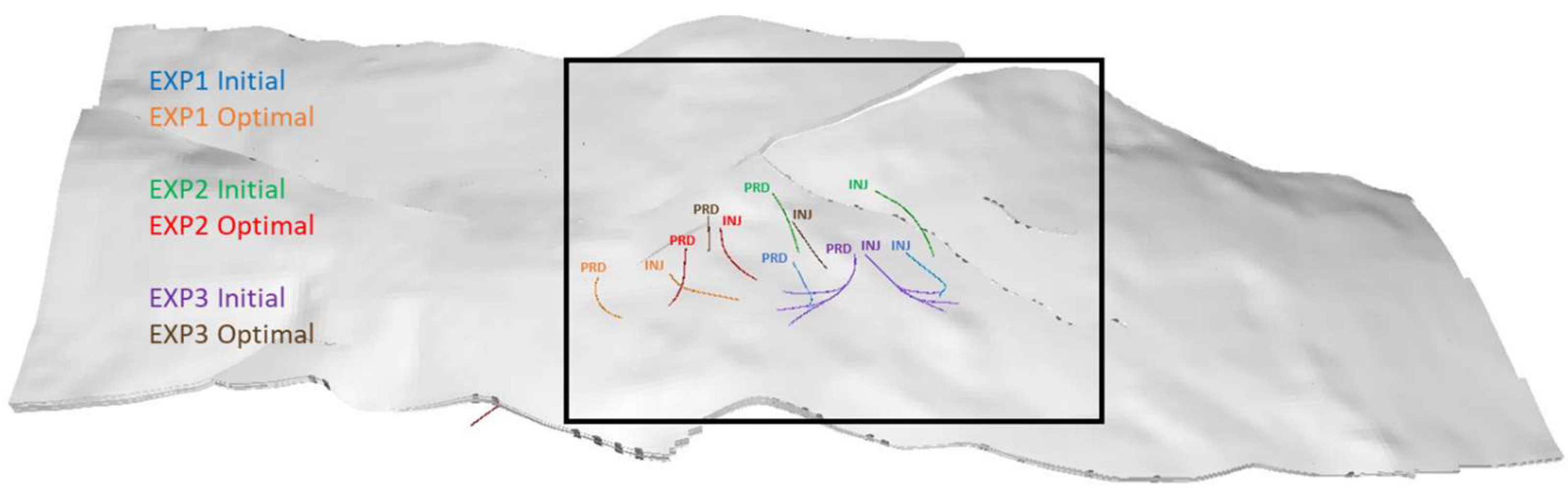
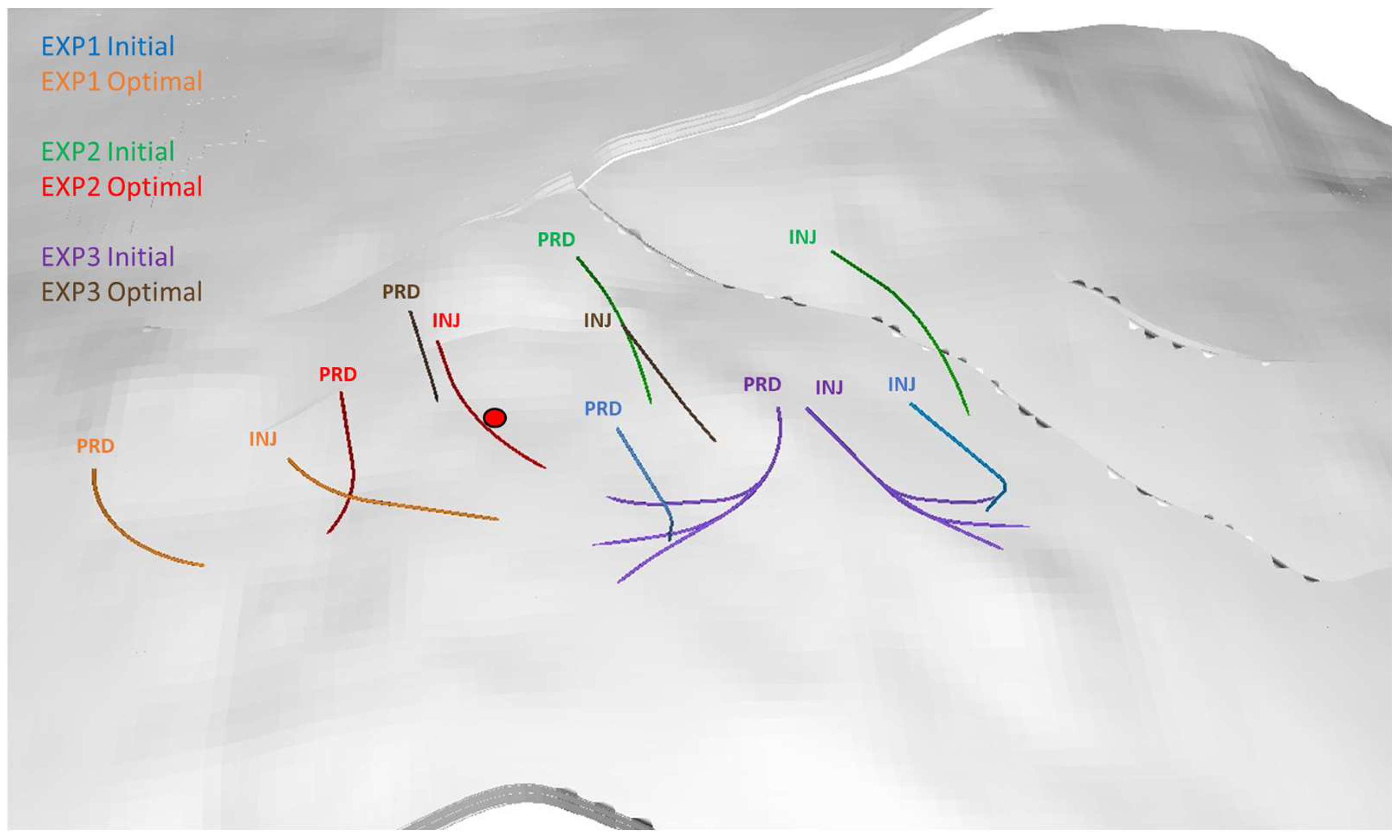
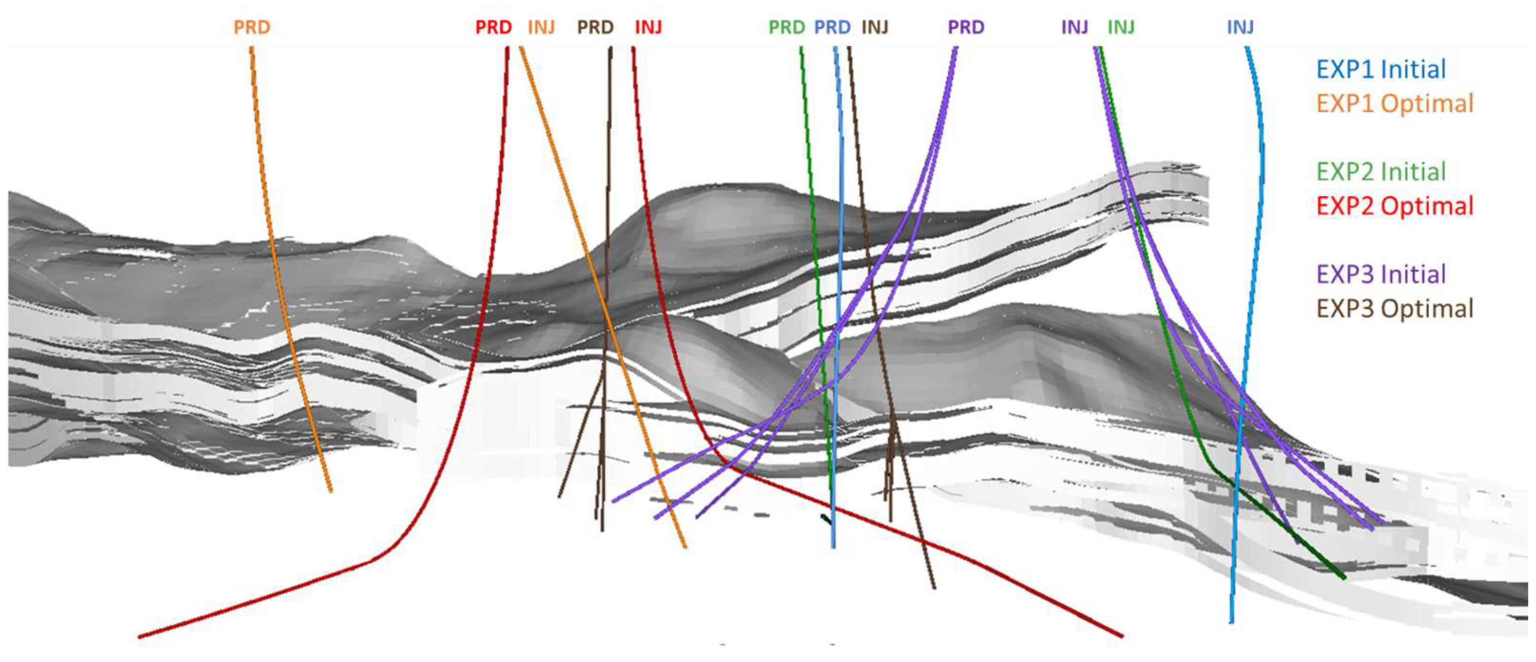
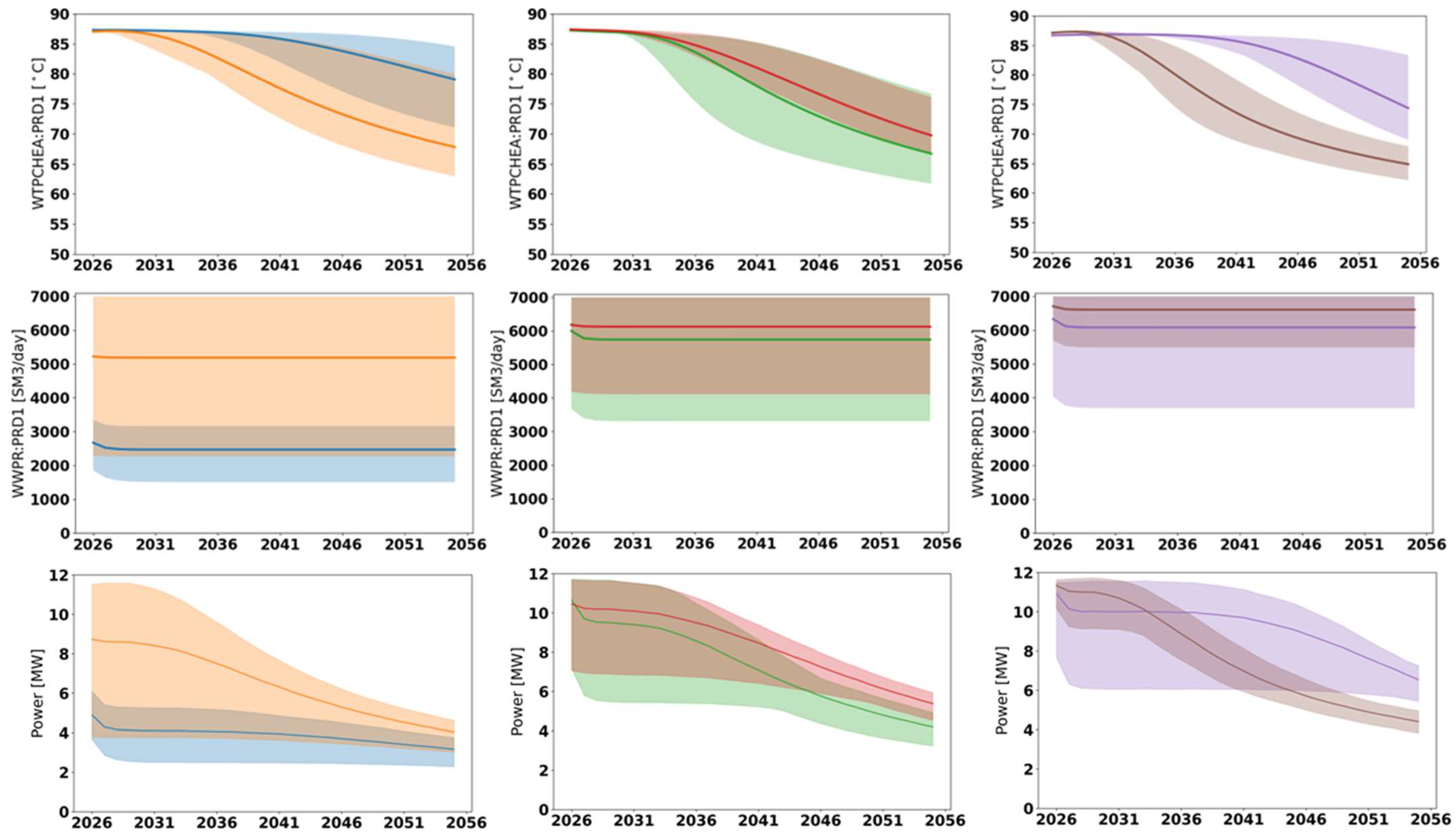
4. Results

4.1. Optimization Experiments

Three numerical experiments have been performed in which well locations/trajectories have been optimized with different initial well concepts: sub-vertical, sub-horizontal and multi-lateral wells. In the first two of the experiments, the optimization has more freedom to explore broadly different types of well shapes (from almost-horizontal to almost-vertical). In Experiment 1, we start with sub-vertical wells. In Experiment 2, we start with sub-horizontal wells. In Experiment 3, we consider multi-lateral wells with two additional legs in addition to the main branch (i.e., three branches in total) of both the injector and the producer. The search space for the shape of multi-lateral wells is constrained by imposing a maximum allowed inclination of 60° for each of the branches (verified for every segment of high-resolution interpolated points of the well trajectory). The starting point of all experiments regarding the location and distance between the injector and producer in the reservoir has been kept similar, i.e., ~1000 m spacing between wells placed right below the fixed surface drilling location. During the optimization, in addition to other economic costs of the project, we also take into account the variable cost per length of each well. In case of multi-lateral wells, this means the sum of the cost of the main branch and the cost of the lateral branches by calculations based on the total combined well length. The initial well locations and trajectories are shown in Figure 7, Figure 8 and Figure 9.

We notice that the optimal locations for the wells for all the three experiments follow a pattern by moving in the same (westerly) direction (Figure 7, Figure 8 and Figure 9) while remaining within the range of feasible outstep from the defined surface drilling location. However, the shapes of the optimized well trajectories differ considerably across the experiments. When starting with sub-vertical wells (Experiment 1), trajectories for both wells stay slightly deviated. On the other hand, when starting with sub-horizontal wells (Experiment 2) and providing more freedom for the well shape to change throughout the optimization, we observe differences in optimal well shapes. Only the trajectory of the producer becomes more vertical, while the shape of the injector remains strongly deviated, as in the initial guess in order to sustain a sufficiently high injection rate (affected by the higher viscosity of cold water) to meet the production rate. For the experiment with multi-lateral wells, the optimal branches are closer to being vertical, and the tie-in point is deeper due to constraint on maximum inclination for each leg.

The optimized doublet configurations in all experiments lead to a noticeable increase in average NPV values (ranging between EUR +4 and +10 million across experiments) and a decrease in LCOE (from 7 to 9 EURct/kWh to 5 EURct/kWh), based on the assumed economic parameters. The highest NPV and lowest LCOE on average (over the ensemble of geological realizations) are achieved by the optimal solution for multi-lateral wells, with slightly worse average values obtained with the optimized sub-horizontal wells (Figure 10). However, the spread or uncertainty on both NPV and LCOE associated with the optimal solution for multi-lateral wells (Experiment 3) is the lowest, even though reducing this spread was not explicitly defined as an objective of the optimization. If we compare the NPV and LCOE of the initial solution of all experiments (also summarized in

Table 2. Overview of optimization results for the three considered well concepts.

	Average NPV (EUR Million)			Min-Max Spread NPV (EUR Million)
Well Concept	Initial	Optimal	Increase	Initial	Optimal
sub-vertical	−5.91	−1.37	4.54	2.73	5.88
sub-horizontal	−4.73	−0.78	3.95	6.11	3.53
multi-lateral	−10.8	−0.55	10.25	5.21	1.91
	Average LCOE (EURct/kWh)			Min-Max spread LCOE (EURct/kWh)
Well Concept	Initial	Optimal	Increase	Initial	Optimal
sub-vertical	8.88	5.59	3.29	4.86	3.92
sub-horizontal	6.52	5.26	1.25	3.36	1.37
multi-lateral	7.95	5.14	2.81	3.87	0.65

), we can also see that an improvement is achieved by simply switching from sub-vertical to sub-horizontal wells; however, this improvement is significantly lower compared to the improvement found by any of the optimization experiments. This provides evidence that it is not only the shape of wells, but the combination of well shape and location that determines the techno-economic performance of the doublet. For multi-lateral wells, the initial solution is less economical due to higher drilling costs, i.e., the achieved well rate and production temperature for initial solution are comparable or better than initial solutions of the other two experiments (Figure 11).

The resulting water injection/production rate, production temperature and generated power generation profiles over time (all calculated by the reservoir simulator) have significant impacts on the project economics. We note that optimization in Experiment 1 (with sub-vertical wells) was able to increase injectivity mostly by finding better well locations. This, however, resulted in a significantly earlier arrival of the cold water front in the producer (Figure 11). In Experiment 2 (initial guess with longer sub-horizontal wells), we started with better injectivity; however, this was also with the earlier cold water breakthrough in the producer. In that scenario, optimization was able to improve upon both aspects (i.e., delaying the arrival of the cold water in the producer and increasing injection/production well rates) by simultaneously determining optimal well locations (including well distance) and adjusting well trajectory shapes. For multi-lateral wells (Experiment 3), we start with relatively high injectivity and late cold water breakthrough. However, in optimal solutions, the increased injectivity comes at the cost of the earlier cold water breakthrough. The generated power profiles of the optimal solutions of each experiment show that optimization favors early power generation, which leads to a higher NPV of the project due to the effects of the assumed discounting factor and the subsidized heat price scheme. These results also show that, despite leading to similar expected NPV and LCOE values for the project, the optimized multi-lateral solution allows for a more aggressive heat power generation than the optimized sub-horizontal at early times (i.e., first 5–7 years). This comes at the expense of a faster decline in heat power generation (driven by the earlier cold water breakthrough) for the optimized multi-laterals when compared to the optimized sub-horizontal case.

4.2. Discussion

One of the main benefits of employing computer-assisted workflows is associated with the reduction in turnaround time to achieve optimized solutions, taking into account a large number of variables and scenarios. The optimization experiments performed for the different well concepts converged in 26, 31 and 32 iterations. Each iteration consisted of 50 flow simulations (one simulation for each geological scenario) to evaluate the current strategy and 50 flow simulations to compute the gradient. This amounts to a total of 2600, 3100 and 3200 reservoir simulations for each experiment, respectively, which, in our case, could be distributed in a high-performance computing server and make the total calculation time equivalent to the simulation runtime of 26, 31 and 32 flow simulations of the Zwolle reservoir model. Since there is a very large number of significantly different well locations and well trajectories, and a large set of geological realizations, an engineering-based optimization approach based on the manual evaluation of all possible strategies is computationally infeasible.

In addition, before drawing conclusions from this study, it is important to underline that the presented results are subject to the assumptions and limitations of the current approach. Besides serving as a reflection on how to appraise the applicability of the reported results, a discussion of these points also provides an outlook of research topics towards further improvements and refinement in the proposed approach to better mirror real-life practical considerations for supporting well concept selection decisions. We highlight the following aspects:

• The optimization experiments performed in this study assume a certain production rate target for the doublet, which was selected based on realistically achievable volumetric rates for the considered reservoir setting with typical wellbore equipment (e.g., completions and ESPs). The obtained results point to the fact that the defined target limit could be too constraining for the case with multi-lateral wells. Future studies should consider investigating the sensitivity of these results to a broader range of realistically achievable rate targets by multi-lateral wells.
• The pressure drop along the well section within the reservoir has not been taken into consideration in this study. This could be included in future studies by activating the multi-segment well option in the OPM-Flow reservoir simulator used here. Depending on flow rate conditions and wellbore geometrical characteristics (e.g., diameter, roughness), this effect could be important, especially for long sub-horizontal wells and multi-lateral well branches.
• Three cases have been considered where both wells of the doublet followed the same well concept, but in principle it would be possible to have cases where the producer and injector have different concepts (e.g., a sub-horizontal producer with a multi-lateral injector).
• The case with multi-lateral wells has assumed multi-laterals with three branches, but in a more general case, the number of branches is also a choice to be made, and therefore potentially an additional variable to optimize.
• While the techno-economic performance of the various well concepts has taken into account the production response of the reservoir, the wellbore stability risks (potentially different for each well concept and well geometry) have not been quantified. If such risks can be modeled and more detailed drilling constraints can be defined, the optimization framework could then be extended to a more holistic and realistic exercise for searching for well designs that satisfy both production and wellbore stability aspects.

5. Conclusions

An optimization-based comparative framework has been proposed to support geothermal practitioners in selecting well concepts. The framework relies on modern state-of-the-art technology for well trajectory optimization under uncertainty. Our existing well trajectory computational workflow has been extended to include the parametrization of multi-lateral wells. Three well concepts (sub-vertical, sub-horizontal and multi-lateral) have been compared for a geothermal doublet planned to be drilled in the West Netherlands Basin based on the optimization results. Geological uncertainty was taken into account by an ensemble of model realizations capturing various scenarios of flow properties of the target reservoir formation.

The main observations derived from the results of the performed experiments in the presented case study are as follows:

• For each well concept, optimization allowed us to significantly improve the techno-economic performance of the doublet system in the Zwolle site by changing the locations and trajectories of both wells (see Table 2).
• Optimized doublet configurations led to a decrease in LCOE from 6.5–9 EURct/kWh to 5–5.5 EURct/kWh, based on the considered economic assumptions.
• The optimized well locations are significantly different to the ones from the engineering-based initial guess and reveal a trend in the location of optimal development areas. This suggests that it is not only the well concept (i.e., the shape or type of wells), but the combination of well concept and well location that determine the techno-economic performance of the doublet.
• The optimized subsurface targets are considered reachable through drilling from the designated surface location.
• Sub-horizontal and multi-lateral well concepts are the most suitable, outperforming the sub-vertical choice in this case.
• The sub-horizontal and multi-lateral concept resulted in similar NPV and LCOE on average across the geological realizations; however, the multi-lateral solution delivers the lowest economic risk (reduced spread in NPV and LCOE).

The approach presented in this paper showcases the added value of optimization technology as a means of improving current best-practices in geothermal field development planning. By accounting for the impact of geological uncertainty while exploring a broad range of well shapes, locations and concepts, the numerical optimization workflow can facilitate and expedite the work of reservoir engineers tasked with identifying the most suitable well solutions in terms of expected performance, feasibility and robustness. By automating the computational steps typically performed manually by engineers when evaluating several scenarios, the workload is shifted towards the analysis and interpretation of the reservoir response, which contributes to a faster turnaround time for a better understanding of the subsurface behavior and improved decisions.

References

- Smith, D.P. Fitting geothermal energy into the energy transition. Neth. J. Geosci. 2019, 98, e6. [Google Scholar] [CrossRef]
- Yang, T.; Liu, W.; Kramer, G.J.; Sun, Q. Seasonal thermal energy storage: A techno-economic literature review. Renew. Sustain. Energy Rev. 2021, 139, 110732. [Google Scholar] [CrossRef]
- European Technology and Innovation Platform on Geothermal (ETIP-G). Strategic Research and Innovation Agenda. 2023. Available online: https://etip-geothermal.eu/front/wp-content/uploads/SRIA_2023_Final_ForWeb_compressed.pdf (accessed on 15 September 2024).
- Van Wees, J.D.; Kronimus, A.; van Putten, M.; Pluymaekers, M.P.D.; Mijnlieff, H.; van Hooff, P.; Obdam, A.; Kramers, L. Geothermal aquifer performance assessment for direct heat production—Methodology and application to Rotliegend aquifers. Neth. J. Geosci. 2012, 91, 651–665. [Google Scholar] [CrossRef]
- Van Wees, J.D.; Veldkamp, H.; Brunner, L.; Vrijlandt, M.; de Jong, S.; van Langen, C.; Heijnen, N.; Peijster, J. Accelerating geothermal development with a play-based portfolio approach. Neth. J. Geosci. 2020, 99, e5. [Google Scholar] [CrossRef]
- Vrijlandt, M.; Struijk, E.L.M.; Brunner, L.H.; Veldkamp, J.G.; Witmans, N.; Maljers, D.; van Wees, J.D. ThermoGIS update: A renewed view on geothermal potential in the Netherlands. In Proceedings of the European Geothermal Congress, The Hague, The Netherlands, 11–14 June 2019. [Google Scholar]
- Yeten, B.; Durlofsky, L.J.; Aziz, K. Optimization of Nonconventional Well Type, Location, and Trajectory. SPE J. 2003, 8, 200–210. [Google Scholar] [CrossRef]
- Jesmani, M.; Bellout, M.C.; Hanea, R.G.; Foss, B.A. Well placement optimization subject to realistic field development constraints. Comput. Geosci. 2016, 20, 1185–1209. [Google Scholar] [CrossRef]
- Barros, E.G.D.; Chitu, A.; Leeuwenburgh, O. Ensemble-based well trajectory and drilling schedule optimization—Application to the Olympus benchmark model. Comput. Geosci. 2020, 24, 2095–2109. [Google Scholar] [CrossRef]
- Akın, S.; Kok, M.V.; Uraz, I. Optimization of well placement geothermal reservoirs using artificial intelligence. Comput. Geosci. 2010, 36, 776–785. [Google Scholar] [CrossRef]
- Ansari, E.; Hughes, R.; White, C.D. Well Placement Optimization for Maximum Energy Recovery from Hot Saline Aquifers. In Proceedings of the 39th Workshop on Geothermal Reservoir Engineering, Stanford, CA, USA, 24–26 February 2014. [Google Scholar]
- Chen, M.; Tompson, A.F.B.; Mellors, R.J.; Abdalla, O. An efficient optimization of well placement and control for a geothermal prospect under geological uncertainty. Appl. Energy 2015, 137, 352–363. [Google Scholar] [CrossRef]
- Zhang, S.; Jiang, Z.; Zhang, S.; Zhang, Q.; Feng, G. Well placement optimization for large-scale geothermal energy exploitation considering nature hydro-thermal processes in the Gonghe Basin, China. J. Clean. Prod. 2021, 317, 128391. [Google Scholar] [CrossRef]
- Schulze-Riegert, R.; Davies, R.; Coronado, J.; Hug, C.; Joonnekindt, J.P.; Mulyani, S.; Pradana, A.; Intani, R.G.; Golla, G.; Gunderson, R.; et al. Well Placement Optimization for Geothermal Reservoir Under Subsurface Uncertainty. In Proceedings of the ECMOR 2022, The Hague, The Netherlands, 5–7 September 2022. [Google Scholar] [CrossRef]
- Hui, G.; Chen, Z.; Schultz, R.; Chen, S.; Song, Z.; Zhang, Z.; Song, Y.; Wang, H.; Wang, M.; Gu, F. Intricate unconventional fracture networks provide fluid diffusion pathways to reactivate pre-existing faults in unconventional reservoirs. Energy 2023, 282, 128803. [Google Scholar] [CrossRef]
- Szklarz, S.P.; Barros, E.G.D.; Khoshnevis Gargar, N.; Peeters, S.H.J.; van Wees, J.D.; van Pul-Verboom, V. Geothermal field development optimization under geomechanical constraints and geological uncertainty: Application to a reservoir with stacked formations. Geothermics 2024, 123, 103094. [Google Scholar] [CrossRef]
- Schulte, D.O.; Arnold, D.; Geiger, S.; Demyanov, V.; Sass, I. Multi-objective optimization under uncertainty of geothermal reservoirs using experimental design-based proxy models. Geothermics 2020, 86, 101792. [Google Scholar] [CrossRef]
- Babaei, M.; Norouzi, A.M.; Nick, H.M.; Gluyas, J. Optimisation of heat recovery from low-enthalpy aquifers with geological uncertainty using surrogate response surfaces and simple search algorithms. Sustain. Energy Technol. Assess. 2022, 49, 101754. [Google Scholar] [CrossRef]
- Fonseca, R.M.; Chen, B.; Jansen, J.D.; Reynolds, A.C. A stochastic simplex approximate gradient (StoSAG) for optimization under uncertainty. Int. J. Numer. Methods Eng. 2017, 109, 1756–1776. [Google Scholar] [CrossRef]
- Lu, R.; Forouzanfar, F.; Reynolds, A.C. Bi-Objective Optimization of Well Placement and Controls Using StoSAG. In Proceedings of the SPE Reservoir Simulation Conference, Montgomery, TX, USA, 20–22 February 2017. [Google Scholar] [CrossRef]
- Chen, B.; Reynolds, A.C. CO2 water-alternating-gas injection for enhanced oil recovery: Optimal well controls and half-cycle lengths. Comput. Chem. Eng. 2018, 113, 44–56. [Google Scholar] [CrossRef]
- Hanea, R.G.; Bjorlykke, O.P.; Hashmi, Y.; Feng, T.; Fonseca, R.M. Robust Multi-Objective Field Development Optimization for the Mariner Asset. In Proceedings of the SPE Reservoir Simulation Conference, Galveston, TX, USA, 10–11 April 2019. [Google Scholar] [CrossRef]
- Barros, E.G.D.; Fonseca, R.M.; de Moraes, R.J. Production optimisation under uncertainty with automated scenario reduction: A real-field case application. In Proceedings of the SPE Reservoir Characterisation and Simulation Conference and Exhibition, Abu Dhabi, United Arab Emirates, 17–19 September 2019. [Google Scholar] [CrossRef]
- Barros, E.G.D.; Ruan, P.; Ishmuratov, R.; Hopman, J.; Fonseca, R.M. Hydraulic fracture stage design optimization of a dry gas field in the North Sea. In Proceedings of the EAGE 2020 Annual Conference & Exhibition Online, 18–20 December 2020. [Google Scholar] [CrossRef]
- Barros, E.G.D.; Szklarz, S.P.; Khoshnevis Gargar, N.; Hopman, J.; Zirotti, G.; Bascialla, G.; Ramsay, T.S.; Fonseca, R.M. Field Development Optimization with Stochastic Gradient Method: Application to a Multi-Reservoir Carbonate Field in the Middle East. In Proceedings of the SPE Reservoir Characterisation and Simulation Conference and Exhibition, Abu Dhabi, United Arab Emirates, 24–26 January 2023. [Google Scholar] [CrossRef]
- Barros, E.G.D.; Szklarz, S.P.; Hopman, J.; Hopstaken, K.; Gonçalves da Silva, J.P.; Bjørlykke, O.P.; Rios, V.; Videla, J.; Oliveira, R.; Hanea, R.G. Well Swapping and Conversion Optimization Under Uncertainty Based on Extended Well Priority Parametrization. In Proceedings of the Offshore Technology Conference Brasil, Rio de Janeiro, Brazil, 24–26 October 2023. [Google Scholar] [CrossRef]
- Chen, Y.; Oliver, D.S.; Zhang, D. Efficient ensemble-based closed-loop production optimization. SPE J. 2009, 14, 634–645. [Google Scholar] [CrossRef]
- Taylor, H.L.; Mason, M.C. A Systematic Approach to Well Surveying Calculations. SPE J. 1972, 12, 474–488. [Google Scholar] [CrossRef]
- Gaupp, R.; Okkerman, J. Reservoir quality of Rotliegend sandstones in the northern Netherlands-A review. In The Permian Rotliegend of the Netherlands; Grötsch, J., Gaupp, R., Eds.; SEPM Society for Sedimentary Geology: Tulsa, OK, USA, 2011; pp. 193–228. [Google Scholar]
- Henares, S.; Bloemsma, M.R.; Donselaar, M.E.; Mijnlieff, H.F.; Redjosentono, A.E.; Veldkamp, H.G.; Weltje, G.J. The role of detrital anhydrite in diagenesis of aeolian sandstones (Upper Rotliegend, The Netherlands): Implications for reservoir-quality prediction. Sediment. Geol. 2014, 314, 60–74. [Google Scholar] [CrossRef]
- Bruijnen, P.; Leewis, M. RESULT-D4.1: 3D Reservoir Characterization Model for Zwolle, 2022.
- Rasmussen, A.F.; Sandve, T.H.; Bao, K.; Lauser, A.; Hove, J.; Skaflestad, B.; Klöfkorn, R.; Blatt, M.; Rustad, A.B.; Sævareid, O.; et al. The Open Porous Media Flow reservoir simulator. Comput. Math. Appl. 2021, 81, 159–185. [Google Scholar] [CrossRef]