Article

System Analysis and Comparison Between a 2 MW Conventional Liquid Cooling System and a Novel Two-Phase Cooling System for Fuel Cell-Powered Aircraft

1
NLR—Royal Netherlands Aerospace Centre, 1059 CM Amsterdam, The Netherlands
2
Airbus Commercial Aircraft, 22335 Hamburg, Germany
3
Aerostack GmbH, 72581 Dettingen, Germany
*
Author to whom correspondence should be addressed.
Energies 2025, 18(4), 849; https://doi.org/10.3390/en18040849
Submission received: 28 November 2024 / Revised: 15 January 2025 / Accepted: 23 January 2025 / Published: 11 February 2025
(This article belongs to the Section D: Energy Storage and Application)

Abstract

:
Hydrogen-powered fuel cells are the preferred energy source for electric aircraft. However, for aircraft applications, it is of upmost importance to reduce the mass of the fuel cell system. A considerable amount of the total system mass is due to the fuel cell cooling system. In this paper, the analysis of a 2 MW cooling system for fuel cell-powered aircraft is discussed. A detailed comparison is made between a conventional liquid cooling system with ethylene glycol–water (EGW) and a novel two-phase cooling system that uses the evaporation of a liquid to remove waste heat from the fuel cells. For this novel two-phase cooling system, several refrigerants were analyzed, and methanol resulted in the lowest system mass. The mass of a liquid EGW system is 35% higher than for two-phase methanol with accumulator and 2.4 times higher than for two-phase methanol without accumulator. Because of this large mass benefit, a demonstrator for a two-phase methanol cooling system without accumulator with a capacity of 200 kW is currently being built.

1. Introduction

1.1. Background

Hydrogen energy holds significant potential in clean energy transition and is an effective pathway for achieving large-scale deep decarbonization in areas such as transportation, industry, and construction [1]. Proton exchange membrane (PEM) fuel cells transform the chemical energy liberated during the electrochemical reaction of hydrogen and oxygen to electrical energy [2]. Fuel cells can operate at a higher efficiency than hydrogen gas combustion turbine engines, and because of the relatively low operating temperature (<120 °C) compared to hydrogen combustion engines, they only exhaust water and no NOx emissions. Hydrogen-powered PEM fuel cells are therefore the preferred energy source for electric aircraft [3]. In the EU-funded BRAVA (Breakthrough Fuel Cell Technologies for Aviation) project [4], technologies for a fuel cell-based power generation System for aviation are being developed for aircraft capable of carrying up to 100 passengers on distances of up to 1000 nautical miles. One of these technologies is the cooling system for the fuel cells. In this paper, the analysis of the 2 MW cooling system is discussed.

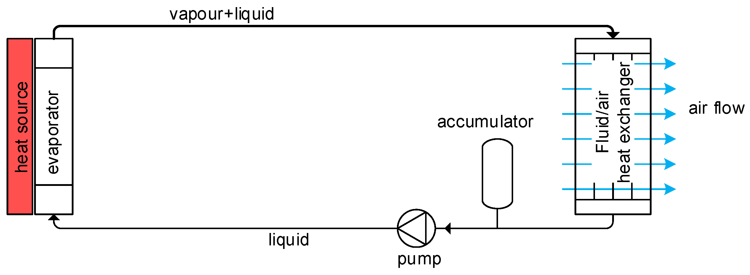
1.2. What Is a Two-Phase Pumped Cooling System?

A fuel cell system generates a significant amount of waste heat that has to be removed with a cooling system, and this cooling system represents a significant part of the total system mass. For this reason, it is of utmost importance to minimize the mass of the cooling system. This can be achieved by using a two-phase cooling (2-PC) system. Originally, 2-PC systems were developed for space applications, for example, for the thermal control system of the Alpha Magnetic Spectrometer (AMS-02) that is mounted on the International Space Station [5]. Also, commercial spacecraft from Thales Alenia Space have 2-PC systems [6], and they have also been developed for active antennae for communication satellites [7]. More recently, 2-PC systems have been developed for cooling power electronics modules in electric aircraft motors [8,9]. Figure 1 shows a schematic drawing of a 2-PC system. A pump transports liquid to an evaporator, which consists of cooling plates that are integrated in the fuel cell stack. In the evaporator, the waste heat from the fuel cells is absorbed and the liquid (partly) turns into vapor (i.e., the term “two-phase” refers to the phase transition of the fluid from liquid to vapor). The vapor/liquid mixture then flows to the condenser. In the condenser, the absorbed heat from the fuel cell (FC) is transferred to the air that flows through the ram air heat exchanger (HX), and the vapor is turned back into liquid. The saturation temperature in the system depends on the pressure, and this pressure is controlled by the accumulator [7,8,9]. The accumulator also allows for fluid density changes (e.g., as a result of evaporation) in the loop.
The schematic of a 2-PC system is very similar to that of the liquid ethylene glycol–water (EGW) cooling system that is commonly used for fuel cells, except that in 2-PC, the liquid is evaporated. This results in several advantages:
  • The required mass flow is an order of magnitude smaller. This results in much lower electrical power consumption of the pump and a much smaller pump mass. Also, the piping diameter can be smaller, which reduces the overall mass of the system.
  • Freezing of the fluid under low ambient temperatures (−55 °C) is not possible, since the freezing points of fluids that are used for two-phase cooling are much lower (typically lower than −80 °C) than the freezing point of EGW (approximately −45 °C).
  • Due to the low freezing point and high heat transfer coefficient of two-phase fluids, it is easier to use the waste heat from the fuel cell to warm liquid H2 before it enters the fuel cell.
  • The heat transfer coefficient for evaporating or condensing flow is typically much higher than the heat transfer coefficient for liquid flow. This results in a smaller temperature difference between the fluid and the heat exchanger walls
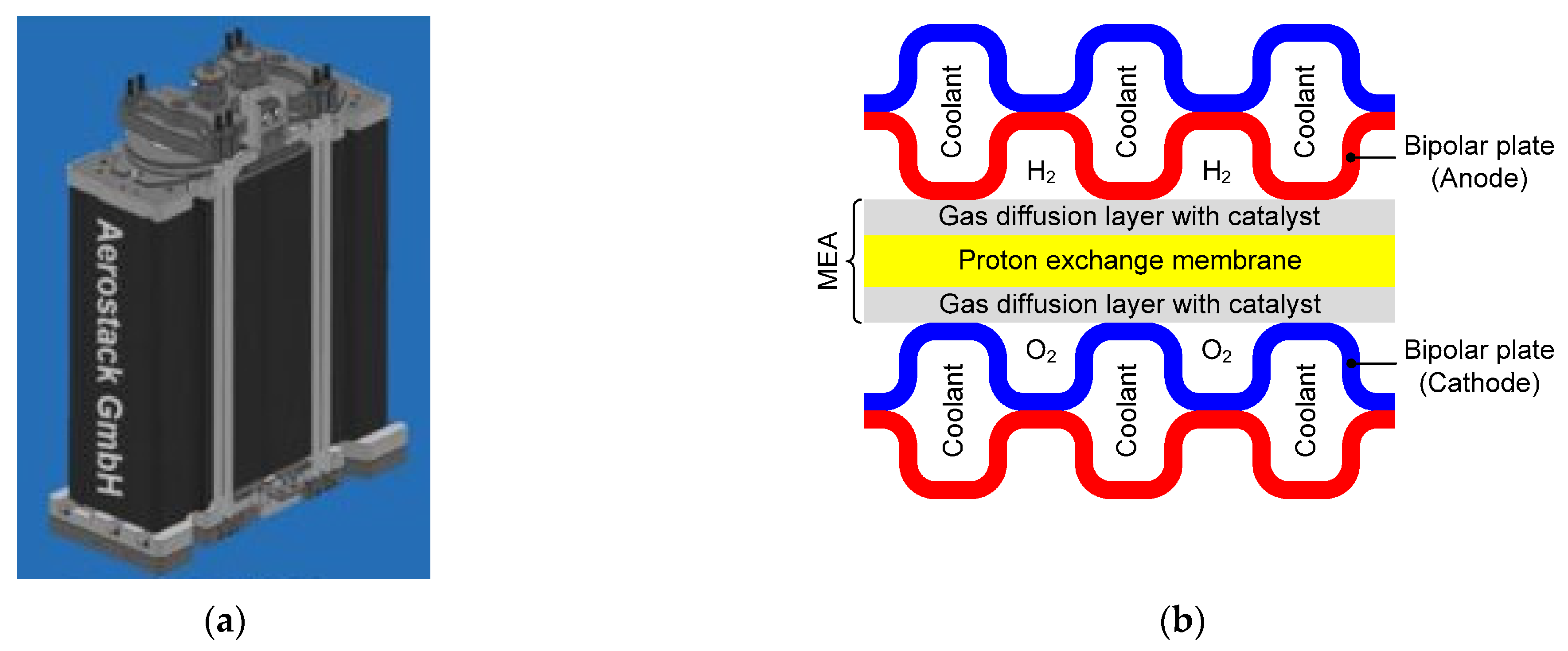
A disadvantage compared to liquid cooling is that the accumulator of a 2-PC system has to be considerably larger. Also, the design is more complex.

1.3. Heat Source

A fuel cell stack (see Figure 2a for a rendering) consists of a large number (around 500) of fuel cells in a membrane electrode assembly (MEA) with metal bipolar plates on either side (see Figure 2b). H2 and O2 gas flow between the MEA and the bipolar plates, while the cooling channels are located between the bipolar plates. Fuel cells typically have an efficiency of ~55%. As a result, 4.4 MW of hydrogen chemical energy results in 2.4 MW fuel cell electrical power and 2 MW of waste heat. The heat flux is typically around 1 W/cm2. Because an FC stack contains a complex system of gaskets and sealings to separate the air, hydrogen, and coolant flows, the pressure of the coolant is limited to approximately 4 barg.
The fuel cell operating temperature has a large influence on its durability and performance [10]. Current PEM fuel cells typically operate at a maximum temperature of 80 °C [2]. In aircraft applications, the air heat exchanger has a large contribution to the total mass of the cooling system. For this reason, there is a strong drive to develop fuel cells that can operate at higher temperatures, since this increases the temperature difference between the cooling fluid and the ambient air, and this reduces the required size and mass of the air heat exchanger. Fuel cells for aircraft applications that can operate at temperatures of 100 °C and a relative humidity below 20% are being developed as part of the BRAVA project [4]. The optimum fuel cell operating temperature for an aircraft application depends on many factors, e.g., the current density [10], the pressure (fuel cell efficiency is typically higher at elevated air pressure, but a higher operating pressure results in a larger air compressor power consumption), and the required size of the humidifier to achieve sufficient relative humidity [4]. The optimum operating temperature is different for different phases (e.g., take-off, climb, cruise) of the flight. Take-off is the most demanding phase for the fuel cell cooling system and it determines the sizing and mass of the system. For the fuel cell system developed in BRAVA, it was determined that the optimum maximum fuel cell coolant temperature during take-off is 95 °C, and this value is used in the analyses discussed in the next sections.
Figure 2. (a) Rendering of a fuel cell stack from Aerostack [11]; (b) cross-section of a single layer in a fuel cell stack [12].
Energies 18 00849 g002

1.4. Heat Sink

The waste heat generated by the fuel cells has to be transported to a heat sink. In electric aircraft, the heat sink is the ambient air outside the aircraft. This air can have a temperature between −55 °C and +50 °C. The air is routed through a ram air heat exchanger. The air is forced through the heat exchanger by the aircraft’s forward motion or, when the aircraft is stationary, by a fan.
When liquid hydrogen (with a temperature of −250 °C) is used as energy carrier in electric aircraft, it has to be warmed to ambient temperatures before it can enter the fuel cell stack. The warming can be achieved with an electric heater, but this costs approximately 8% of the electrical output of the fuel cell. Instead, the liquid hydrogen flow can also be used as an additional heat sink for the waste heat of a fuel cell.

2. Analysis Methods

In this section, the methods for the 2 MW cooling system analyses are discussed. The analysis starts with a fluid preselection. The most promising fluids are then analyzed in more detail, after which the fluid is selected. In the analysis, the 2-PC system is also compared to a conventional cooling system with a liquid EGW mixture.

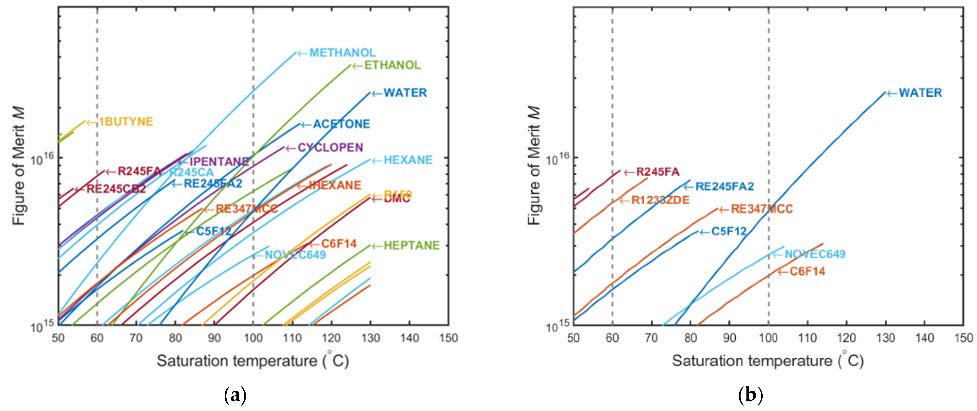
2.1. Fluid Preselection with “Figure of Merit”

For 2-PC, it is important that the tubing has a small diameter. Not only is the routing of the tubing much simpler when the diameter is small, but the system volume also scales with the square of the diameter, and a higher system volume results in a higher fluid mass and larger and heavier components. For this reason, it is important to minimize the diameter of the tubing. However, a small diameter of the tubing results in a large pressure drop. This pressure drop is not only disadvantageous for the pump power, but a large pressure gradient in a 2-PC system also results in a large temperature gradient (since pressure and boiling temperature are related). For this reason, an important characteristic of the fluid for 2-PC is a small pressure drop for a certain heat transport and geometry. The pressure drop Δp in tubing is proportional to a fluid-dependent part and a geometry-dependent part (i.e., the length and diameter of a tube), as well as depending on the heat input [13]:
Δ p μ l 1 / 4 ρ l h l v 7 / 4 + μ v 1 / 4 ρ v h l v 7 / 4 fluid   dependent   part L d 19 / 4 geometry P 7 / 4 heat ,
where μ is the fluid viscosity (with subscript l for liquid and subscript v for vapor), ρ is the density, hlv is the heat of evaporation, L is the length of a tube, d the internal diameter, and P the heat input. The pressure gradient in the loop results in a gradient in the saturation temperature in the loop [13]:
Δ T = Δ p T sat p sat μ l 1 4 ρ l h l v 7 4 + μ v 1 4 ρ v h l v 7 4 T sat p sat .
where T sat / p sat is the change in saturation temperature as a result of change in pressure, which is a fluid property (see Table 1 for the values for different fluids). The inverse of the equation above can be used to find a fluid that results in a small temperature gradient (as a result of the pressure gradient). This inverse is called a figure of merit [13]:
M = 1 ( μ l 1 / 4 / ( ρ l h l v 7 / 4 ) + μ v 1 / 4 / ( ρ v h l v 7 / 4 ) ) T / p , figure   of   merit   based   on   low   temperature   gradient
Figure 3a shows this figure of merit M for temperatures between 50 °C and 130 °C for all fluids in the NIST REFPROP [14] fluids database. On the horizontal axis, the saturation temperature of the fluid is shown. The FCs that are being developed in the BRAVA project have an operating temperature between 60 °C and 100 °C. These temperatures are indicated with the dashed grey vertical lines. The pressure of a fluid increases with saturation temperature, and results with a saturation pressure above 5 bara (the maximum pressure for the fuel cell is 4 barg) are excluded, which is the reason why many lines are truncated above a certain temperature.
Methanol has the highest figure of merit, which means that the tubing diameter can be significantly smaller than for other fluids. However, methanol is flammable and toxic. Figure 3 shows the figure of merit with flammable fluids excluded. The best non-flammable fluids that can be used at fuel cell operating temperatures are water, Novec 649, and C6F14 (perfluorohexane, also known as Fluorinert 72). Table 1 shows fluid properties of methanol and these non-flammable fluids. From the figures, it can be seen that methanol has about a 10 times higher figure of merit than, e.g., C6F14. As a result, a 2-PC system with methanol can have smaller tubing diameter than with C6F14, which results in a lower mass of the system. This is further analyzed with the NLR system analysis tool, which is described in the next sections.
The saturation temperature has a large influence on the figure of merit of fluids because the pressure in the system becomes higher with higher saturation temperature, and this higher pressure results in a smaller vapor volume flow, which results in smaller pressure differences. For FCs operating above 120 °C, water becomes a very efficient two-phase fluid. When water is used as a two-phase cooling fluid, it would be possible to dump the water vapor directly into the ambient air during take-off on a hot day, instead of condensing water vapor back into liquid in the ram air HX. This would result in a much smaller ram air HX.
Table 1. Relevant properties at 95 °C for preselected fluids.
Methanol RE347mcc (HFE-7000) Water Novec 649 Fluorinert 72 (C6F14)
NFPA (health/flammability) [15]1-33 1-00-03 1-01-0
Global warming potential ~0530~019300
Saturation pressure at 95 °C (bar) 3.06.00.83.93.1
Saturation pressure at 60 °C (bar) 0.852.40.201.51.1
Saturation pressure at 20 °C (bar) 0.130.590.020.330.24
Triple point (°C)−97−1220−108−86
Heat of evaporation hlv (kJ/kg)103510422707273
Specific heat Cp (kJ/kgK)3.11.44.21.21.2
Liquid density ρl (kg/m3)717118496213611446
Density ratio ρlv2082419152836
Conductivity kl (W/m K)0.190.050.680.050.06
Tsat/∂psat (°C/bar)10.16.831.89.912.2
1 The NFPA health safety classification code of 3 is due to emergency situations where the material may thermally decompose and release hydrogen fluoride. Under normal conditions, HFE-7000 and Novec 649 are non-toxic.

2.2. System Analysis Tool

In the next sections, the fluids listed in Table 2 are further analyzed with the NLR cooling system analysis tool. Also, a system with liquid EGW is analyzed and the calculated mass and power are compared to a those of a 2-PC system. The system analysis software can calculate the steady-state and transient behavior of two-phase and single-phase cooling systems and vapor compression cycles by numerically solving the 1D mass and enthalpy equations. The software also includes a cross-flow air–fluid heat exchanger. A detailed description of the model and the correlations for the pressure difference and heat transfer coefficient that are used in the model can be found in [16,17]. For the analyses, the following requirements are used:
  • Total heat rejection during take-off: 2 MW.
  • Maximum power consumption (fans and pumps): 100 kW.
  • Air temperature during take-off: 30 °C.
In the analyses, the power consumption is kept the same for the different fluids, and the emphasis is on the comparison of the system mass for different fluids.

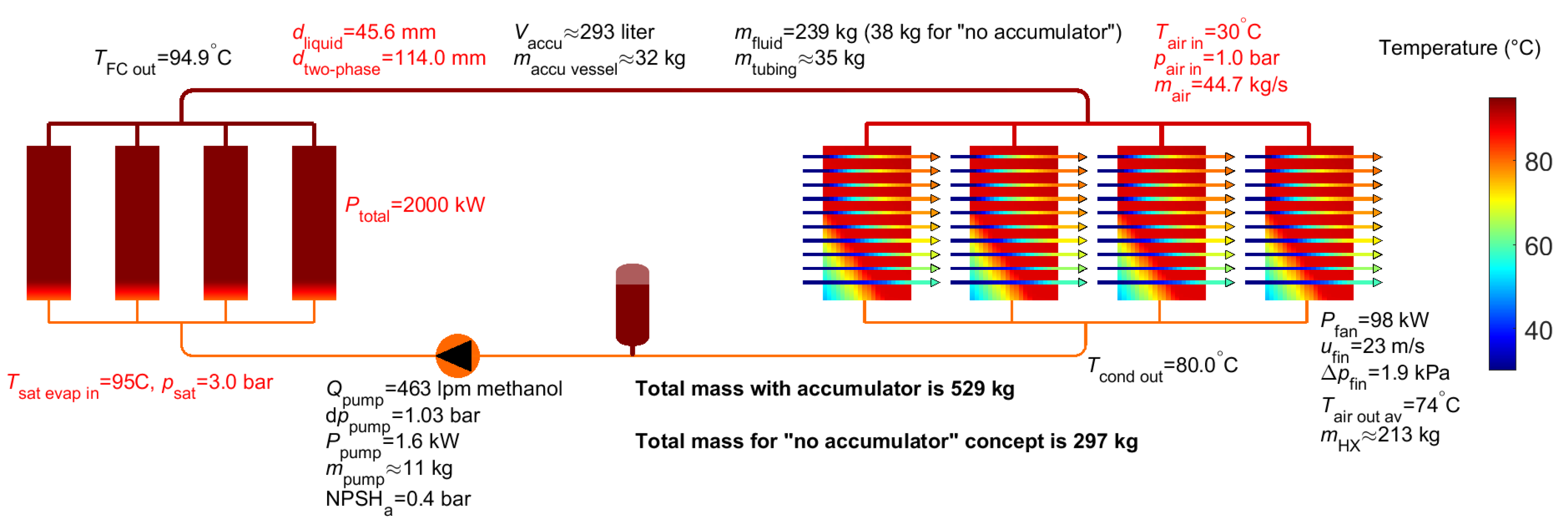
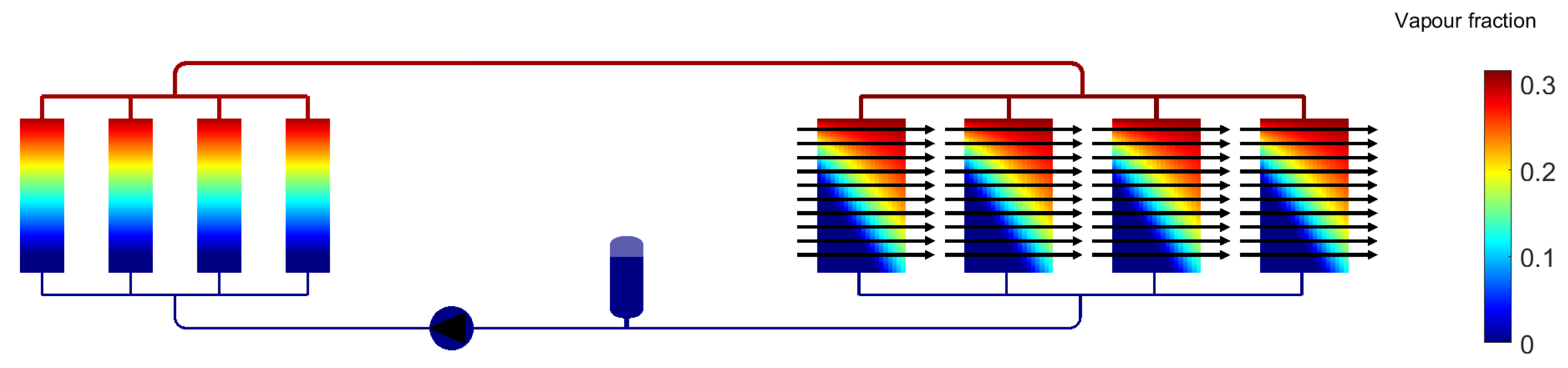
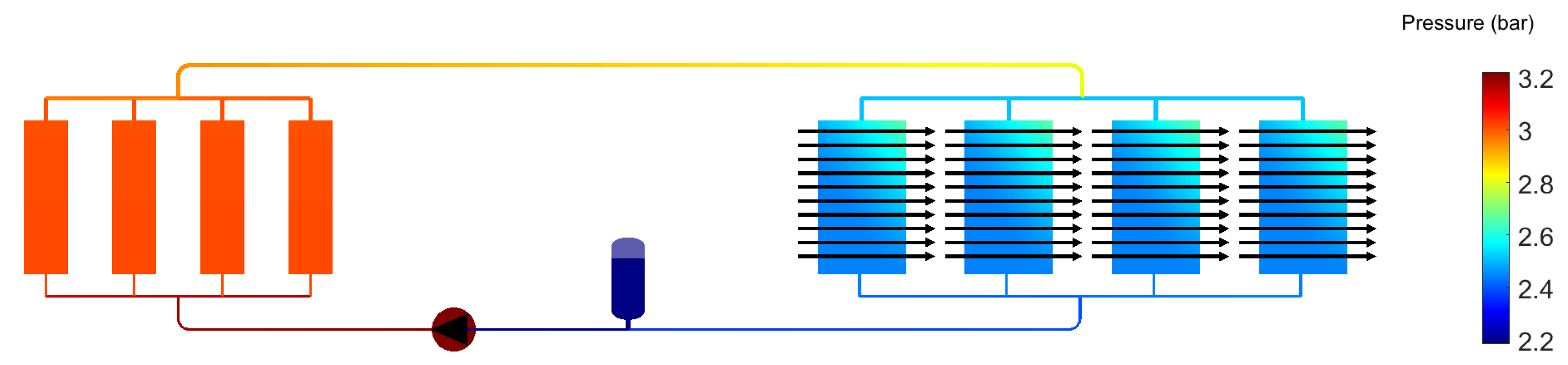
3. Results for Two-Phase Methanol

Figure 4 shows the calculated temperatures in the system for take-off conditions with methanol as coolant. Figure 5 and Figure 6 show the calculated vapor mass fraction and pressure. The input parameters for the model are indicated with red text, while the output is in black text. The mass flow is chosen such that 30% of the liquid is evaporated in the evaporator. All simulation parameters for the analysis are provided in Appendix A.1, while the geometry parameters are provided in Appendix A.2. The system contains four parallel ram air heat exchangers and there are four parallel groups of evaporators. Liquid is pumped to the evaporators, where it absorbs the waste heat from the fuel cells. As a result, the liquid temperature rises until it reaches the saturation temperature, after which the liquid starts to evaporate, and the temperature no longer rises. Instead, the vapor mass fraction increases along the evaporator. The liquid/vapor mixture then flows to the condensers where it condenses back into liquid. The temperature at the condenser inlet is 4 °C lower than the evaporator outlet temperature as a result of the pressure difference between the evaporator and the condenser. This value can be reduced by increasing the diameter of the tubing, but this would increase the volume of the accumulator. The pressure at the inlet of the pump is 2.2 bara. The pump has an inlet temperature of 80 °C, which means that the liquid methanol will start to boil below a pressure of 1.8 bara. The difference between the pump inlet pressure and the pressure at which the fluid starts to boil is called the available NPSH (net positive suction head) for the pump. In order to prevent cavitation of the pump, the available NPSH must be larger than the minimal required NPSH. A typical required NPSH for a centrifugal pump is 0.3 bar, so the available NPSH of 0.4 bar for the system with methanol is sufficient to prevent cavitation of the pump. The total pressure drop over the pump is 1 bar. The pump power is 1.6 kW (assuming a pump efficiency of 50%). The required fan power is 98 kW (assuming a fan efficiency of 75%) and the total fan and pump power is just below the requirement of 100 kW. The mass and size of the air heat exchanger can be made smaller at the expense of higher fan power.
In Appendix B, the details for the mass calculation are provided. The total mass of the fluid (239 kg), tubing (35 kg), accumulator (32 kg), pump (11 kg), and heat exchanger (213 kg) is 529 kg. The mass of the fluid has a large contribution to the total mass of the cooling system. However, only a small fraction of this fluid mass is actually in the loop when the system is operational with a fuel cell heat load, since in that case, a large part of the system volume is filled with vapor and the excess liquid is stored in the accumulator. Conventional pumped two-phase cooling systems have an accumulator, but it is possible to have 2-PC without an accumulator [18]. In that case, the mass flow is scaled with the fuel cell heat load such that the vapor fraction in the system remains approximately constant. Without an accumulator, a very large reduction in system mass could be achieved, not only because of the absent accumulator, but primarily because of the large reduction in fluid mass. The total mass of a 2-PC system without an accumulator is 297 kg (38 kg for fluid, 35 kg for tubing, 11 kg for the pump, and 213 kg for the heat exchanger). In order to investigate the feasibility of a system without an accumulator, a 20 kW 2-PC system with methanol was built and successfully tested [19].

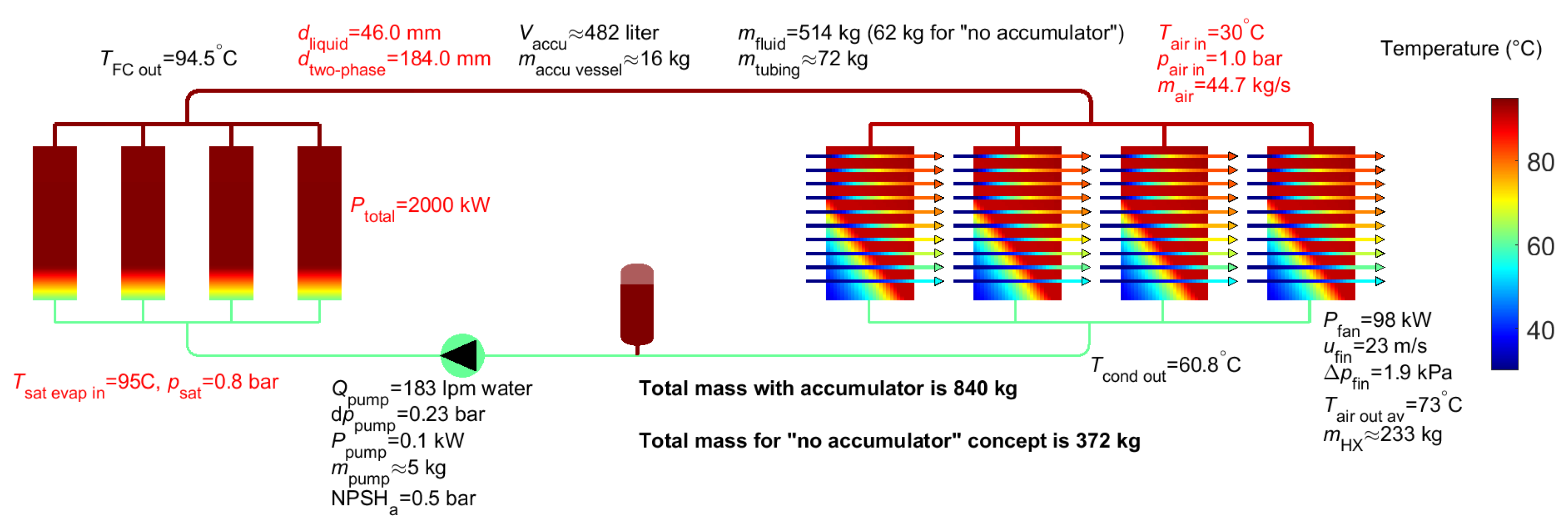
4. Results for Two-Phase Water

Figure 7 shows the calculated temperatures in the system for take-off conditions with water as two-phase coolant. The system parameters and geometry are exactly the same as for the simulation for methanol, except for the following differences:
  • FLUID.name = “water” instead of “methanol” (see Appendix A).
  • constant.d_twophase = 178e-3 instead of 114e-3.
  • constant.d_liquid = constant.d_twophase*0.25 instead of constant.d_liquid = constant.d_twophase*0.4.
Water has a high heat of evaporation (see Table 1), which means that the required water volume flow is very small compared to methanol (183 L/min versus 463 L/min). However, the absolute pressure of water at a boiling temperature of 95 °C is just 0.8 bar, which means that the pressure drop over the system has to be kept relatively small. As a result, the diameter of two-phase tubing has to be larger than for methanol, which results in a higher fluid mass. The total calculated system mass with two-phase water is 840 kg, which is higher than for methanol (529 kg). Water is therefore not a good fluid for two-phase cooling of fuel cells at 95 °C (but it becomes a good fluid > 120 °C).

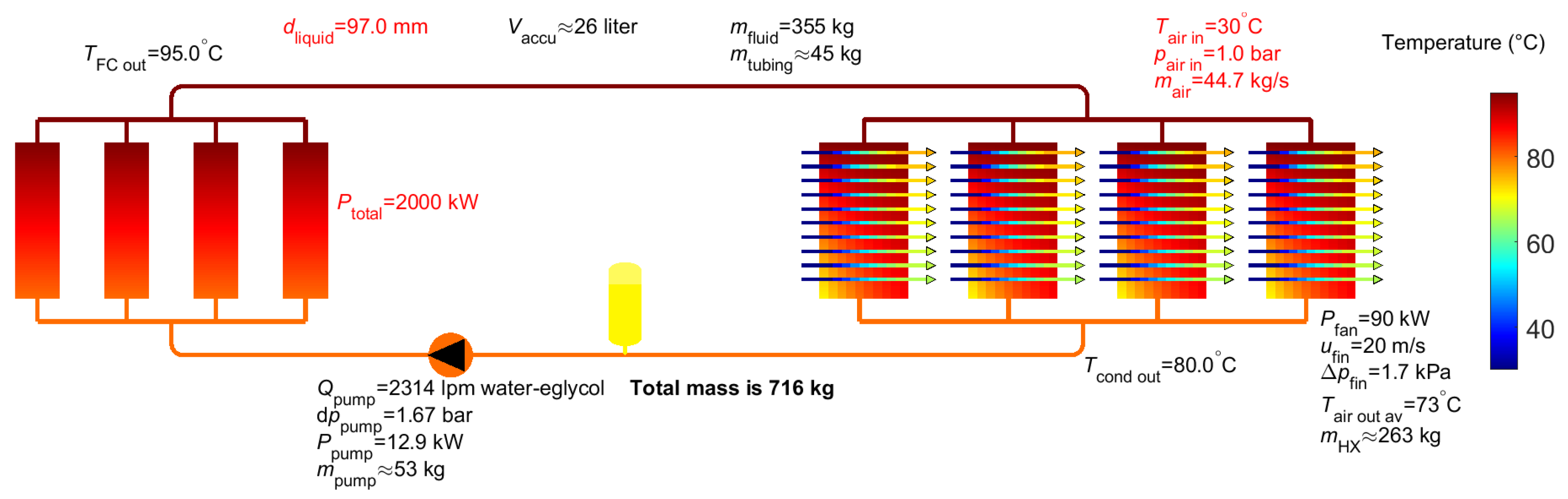
5. Results for Liquid EGW Mixture

In the previous sections, 2-PC systems were analyzed. In this section, a cooling system with a liquid EGW mixture is analyzed. The system parameters and geometry are exactly the same as for the simulation for two-phase methanol, except for the following differences:
  • FLUID.cooling_type = 1 instead of 2 (2 = two-phase cooling, 1 = liquid cooling).
  • FLUID.name = “water-eglycol” (40–60% mixture) instead of “methanol”.
  • constant.d_twophase = 97e-3 instead of 114e-3.
  • The size of the air HX in the direction of the airflow is increased by 10%: HX.L = 0.21*1.1 instead of 0.21.
  • The width of the air HX is increased by 15%: HX.W = 0.75*1.154 instead of 0.75.
Figure 8 shows the calculated temperatures in the system for take-off conditions for a liquid EGW cooling system. The liquid flow for the EGW cooling system is chosen such that the increase in liquid temperature over the fuel cell is 15 °C. The volume flow is five times larger than for a 2-PC with methanol. Also, the pressure drop over the pump is larger. As a result, the required pump power is 12.9 kW compared to 1.6 kW for methanol. Because of the higher pump power, the air HX is made slightly larger in order to decrease the pressure drop over the air HX and thereby reduce the fan power to 90 kW so as not to exceed the 100 kW requirement for the fan + pump by too much. The ram air HX is dimensioned such that the liquid temperature at the exit of the fuel cell is 95 °C, which requires a small increase in the air HX size because the average fluid temperature in the heat exchanger is slightly lower compared to that in 2-PC, and the heat transfer coefficient for liquid EGW is lower than for two-phase methanol.
The inner diameter of the tubing of a liquid EGW system (97 mm) is much larger than the liquid tubing diameter in a 2-PC system with methanol (46 mm) but slightly smaller than the two-phase tubing diameter with methanol (114 mm).
The accumulator for a liquid cooling system can be relatively small (since it only has to compensate for density changes in the liquid due to temperature variations) and the mass of this vessel is neglected in the analysis. For a liquid EGW cooling system, the total mass of the fluid (355 kg), tubing (45 kg), pump (53 kg), and heat exchanger (263 kg) is 716 kg, which is 35% higher than for two-phase methanol with an accumulator (529 kg) and 2.4 times higher than for two-phase methanol without an accumulator (297 kg).

6. Summary of Analysis Results

Table 2 shows the summary of the analysis results. For 2-PC, using methanol results in a system mass of 529 kg for a conventional system and 297 kg for a system without an accumulator. Using a non-flammable alternative results in much higher system mass. A cooling system with a liquid EGW mixture was also analyzed. These results are included in the right column of Table 2. The mass of a liquid EGW system is 716 kg, which is 35% higher than for two-phase methanol with accumulator (529 kg) and 2.4 times higher than for two-phase methanol without an accumulator (297 kg). In order to investigate the feasibility of a system without an accumulator, a 20 kW 2-PC system with methanol was built and successfully tested [19]. The pump volume flow for liquid EGW is five times larger than for two-phase methanol.
Besides the high system mass with the non-flammable fluids Novec 649 and Fluorinert 72, concerns have been raised recently about the environmental impact of PFAS (per- and polyfluoroalkyl substances) [20]. There is currently a proposal from the European Chemical Agency to restrict PFAS, including refrigerants [21]. In this proposal, there are exceptions for the restrictions, e.g., “refrigerants in HVACR-equipment in buildings where national safety standards and building codes prohibit the use of alternatives” and “refrigerants in transport refrigeration other than in marine applications”. However, even if there would be an exception, manufacturers might decide to stop producing this refrigerant anyway. This might impact future availability of Novec 649, Fluorinert 72, or other engineered refrigerants.

7. Discussion

A two-phase methanol cooling system for fuel cells has a significant mass benefit compared to a more traditional liquid EGW cooling system (it has a 2.4 times lower mass when the “no accumulator” concept [19] is used). Also, the pump volume flow is five times lower. There are also some other benefits of using two-phase methanol. For example, when liquefied hydrogen (LH2) is used as an energy source for the fuel cells, it has to be warmed from −250 °C to ambient temperature. This can be achieved with an electric heater, but this costs 8% of the electrical output of the fuel cell. Instead, the waste heat of a fuel cell could also be used to warm the cold hydrogen (only about 10% of the waste heat is required). Using liquid EGW to warm the LH2 is extremely complex, because the freezing point of EGW is relatively high, and the heat transfer coefficient of EGW becomes very low at low temperatures. As a result, a system with liquid EGW is prone to freezing issues. A system with two-phase methanol is much less prone to freezing issues due to two reasons:
  • The freezing point of methanol is lower (−97 °C, see Table 2).
  • In a heat exchanger with two-phase methanol, there is a high heat transfer coefficient between the methanol vapor and liquid, and this prevents the liquid from freezing.
Because of the low freezing point of methanol, it is also possible to use the waste heat from a two-phase methanol cooling system for, e.g., preventing ice formation on the wings.
A two-phase methanol cooling system also has drawbacks. For example, methanol has poor material compatibility with titanium and several aluminum alloys. This can be a large issue, since ram air heat exchangers are made from aluminum. For this reason, material compatibility tests (at 95 °C) with several aluminum alloys (and other materials that are used in a fuel cell cooling system) were carried out as part of the BRAVA project. Although no large issues for material compatibility have materialized so far, thorough compatibility tests (including, e.g., the aluminum solder material) have to be conducted before this technology can be applied in aircraft. Also, the flow distribution over parallel evaporator and condenser branches and gravity effects on the flow distribution can be an issue in poorly designed two-phase cooling systems. For this reason, tests were carried out with a two-phase methanol cooling system with a capacity of 20 kW [19]. The test results from the 20 kW system were used for the design of a two-phase methanol cooling system without accumulator with a cooling capacity of 200 kW, which is currently under construction.

8. Conclusions

In this paper, a two-phase cooling system with a cooling capacity with 2 MW was analyzed. This analysis was used to select methanol as the cooling fluid. Using a non-flammable fluid results in a much higher system mass.
A cooling system with a liquid ethylene glycol–water mixture (EGW) was also analyzed. According to the simulations, the mass of a liquid EGW system is 35% higher than for two-phase methanol with an accumulator and 2.4 times higher than for two-phase methanol without an accumulator. Because of this large mass benefit, a demonstrator for a two-phase methanol cooling system without an accumulator with a capacity of 200 kW is currently being built as part of the BRAVA project.

Author Contributions

Conceptualization, W.R., G.M. and M.-B.B.; methodology, H.J.v.G.; software, H.J.v.G. and T.L.; validation, H.J.v.G.; formal analysis, H.J.v.G.; investigation, H.J.v.G.; resources, H.J.v.G.; data curation, H.J.v.G.; writing—original draft preparation, H.J.v.G.; writing—review and editing, T.L., G.M. and M.-B.B.; visualization, H.J.v.G. and T.L.; supervision, H.J.v.G.; project administration, H.J.v.G.; funding acquisition, H.J.v.G. All authors have read and agreed to the published version of the manuscript.

Funding

The BRAVA project is funded by the European Union’s Horizon program under grant agreement number 10110149. This publication reflects the authors’ views. Neither the European Union nor the Clean Hydrogen Joint Undertaking can be held responsible for them.

Data Availability Statement

The input parameters for the simulations described in this study are included in the Appendix A and Appendix B of this article. Further inquiries can be directed to the corresponding author.

Conflicts of Interest

Authors William Resende and Georg Mühlthaler were employed by the company Airbus Commercial Aircraft. Author Marcus-Benedict Buntz was employed by the company Aerostack GmbH. The remaining authors declare that the research was conducted in the absence of any commercial or financial relationships that could be construed as a potential conflict of interest. The funders had no role in the design of this study; in the collection, analyses, or interpretation of data; in the writing of the manuscript; or in the decision to publish the results.

Appendix A. Input for System Analysis

Appendix A.1. Simulation Parameters

%% Simulation settings
FLUID.cooling_type = 2;   % 2 = two-phase, 1 = liquid
FLUID.name = 'methanol'; % Fluid in system, if mixture (only for liquid cooling): always split by: -
FLUID.mix = [0.4 0.6];    % fraction of mixture (only for liquid cooling): first fraction is for first fluid in FLUID.name
system = 'Airbus';     % Geometry of system

%%Initial values and conditions
constant.P(1:4) = 500e3;  % Heat input per Fuel Cell branch [W]
constant.nrBranch = length(constant.P);% number of evaporator branches
constant.nrCondens = 4;  % number of condensers
constant.nrCondensAir = 20; %non-physical division of condenser in several parallel tubes (for the cross-air heat exchanger).

constant.NRiter = 150;  % NR of iterations
constant.CalcParallel = 0; % if 1, calculate distribution, if 0, assume equal distribution over parallel branches
constant.dP_cor = 1;      % Two-phase frictional pressure drop correlation. 1 = Muller-Steinhagen&Heck, 2 = Friedel

constant.Xexit = 0.3;   % vapour mass fraction after evaporator
constant.DTpreheat = 15;  %For liquid, this is the temperature increase due to the heat load, for two-phase, this determines the preheater power (if present in system)

constant.Tkelvin = 273.15;  % zero degrees Celsius [K]
constant.Tsp = 95 + constant.Tkelvin; % set-point temperature [K]
constant.Tsink = 30 + constant.Tkelvin; % heat sink (i.e. space or ambient air) temperature [K]
constant.Tinit = constant.Tsink;  % initial temperature of the loop [K]

constant.pump_eff = 0.5;  % adiabatic efficiency of pump [-]
constant.fan_eff = 0.75;   % adiabatic efficiency of pump [-]

constant.Recuperator = 0;  % 1 = with recuperator, 0 = without recuperator

%% accu properties
accu.Tmax = 110 + constant.Tkelvin; % maximum temperature used for strength and mass calculation
accu.Hratio = 1.5; % ratio between the height of the cylindrical part and the diameter of the accumulator, e.g., Hratio = H/D
accu.material = 'aluminium';
accu.rho = 2700; % density [kg/m^3]
accu.factor_proof = 3; % factor for proof pressure
accu.factor_burst = 4; % factor for burst pressure
accu.Smargin = 1.25; %additional margin factor for proof and burst calculation
accu.Syield = 83e6; %yield strength [N/m2]
accu.Sultimate = 110e6; %ultimate strength [N/m2]

%% ambient air input
air.InputType = 1; % if InputType = 1, air mass flow is input. if InputType = 2, air mass flow is calculated from air speed
air.m   = 44.7/4; % air massflow [kg/s] (only for air.InputType = 1)
air.U   = 230/3.6; % flight speed in [m/s] (only for air.InputType = 2)
air.pin = 1e5;  % ambient air pressure [Pa]
air.Tin = constant.Tsink; % Ambient air temperature; HX inlet air temperature
air.Tout = air.Tin + 30; % Initial guess for HX outlet air temperature

%% Finned air HX properties
HX.L  = 0.21;   % Length of HX [m]: from air inlet to air outlet
HX.Wlayer  = 0.75*1.03;  % Width of HX layer of fins [m]
HX.NRlayer  = 44;  % number of layers of fins
HX.W = HX.Wlayer*HX.NRlayer;%: width of HX times number of layers of fins
HX.Hfin = 15e-3;   % Height of one fin [m]
HX.tfin = 0.15e-3;  % Thickness of one fin [m]
HX.dfin = 0.82e-3;  % Distance between two fins [m]
HX.k  = 167;    % Thermal conductivity of material btwn condenser-tube and airHX [W/mK]
HX.rho = 2700;    % Density of material btwn condenser-tube and airHX [kg/m3]
HX.K_inlet = 0.0;   % Minor pressure loss at air inlet of HX
HX.K_outlet = 0.0;  % Minor pressure loss at air inlet of HX

Appendix A.2. Geometry Parameters

%########################################################################%
%#                               #%
%#    Geometry of Airbus two-phase cooling MPL          #%
%#                               #%
%########################################################################%
%#                               #%
%# Components are structured like this:                 #%
%# <ID>    = Identifier number                    #%
%# <Name>      = Component name               #%
%# 'L'       = Length of component [m]               #%
%# 'D'        = Diameter of component [m]            #%
%# 'D_restriction' = Diameter of restriction [m], 0 for no restriction       #%
%# 'nParTube'  = Number of parallel tubes [-]              #%
%# 'Shape' = Geometrical shape of tubes. 0 for round, 1 for square      #%
%# 'Diab'    = 0 for none, 1 for evaporator, 2 for HX,          #%
%#          3 for condenser, 4 for single-phase         #%
%# 'mass'    = Mass of component [kg]                #%
%# 'Cp'     = Specific heat of material [J kg-1 K-1]          #%
%# 'K'        = minor loss coefficient               #%
%# 'nElm'    = Number of elements per component           #%
%# 'e'      = Pipe inner roughness                 #%
%########################################################################%

constant.d_twophase = 114e-3; % [m] inner diameter of two-phase tubing
if FLUID.cooling_type = =1
 constant.d_liquid = constant.d_twophase; % [m] inner diameter of liquid tubing
else
 constant.d_liquid = constant.d_twophase*0.4; % [m] inner diameter of liquid tubing
end

d_condenser = 1.4e-3; % [m] inner diameter of condenser tubes

d_factor = constant.d_twophase/114e-3; % scaling factor for diameter of condenser, etc.
restriction_factor = 1;


%% Minor pressure loss constants
% From: Y. A. Çengel, Fundamentals of thermal-fluid Sciences (McGraw-Hill, New York, 2012).
K_elbow = 1.1;
K_union = 0.08;
K_tee_b = 2;  % Branch flow
K_tee_l = 0.9; % Line flow
K_long_bend = 0.3;
K_inlet = 0.5; % inlet loss
K_outlet = 1; % outlet loss


nC = 0;      % Start counting the number of components
%% Tube from pump to Evap
nC = nC + 1;
name = 'Tube_PtoE';
ID.(name) = nC;
C(nC) = struct('ID',name, 'L',5, 'D',constant.d_liquid,'D_restriction',0.0e-3, 'nParTube',1, 'K',K_outlet + K_long_bend*2,'e',2e-6, 'Shape',0, 'Diab',0, 'mass',1, 'Cp',1);

for i = 1:constant.nrBranch %% START evaporator branches

 d_restriction = constant.d_liquid*restriction_factor; % add restriction to inlet of each branch
%d_restriction = 0;
%% tube to Evaporator that contains the restriction
 nC = nC + 1;
 name = 'Tube_toE';
 ID.(name)(i) = nC;
 C(nC) = struct('ID',[name '' int2str(i)], 'L',0.1, 'D',constant.d_liquid,'D_restriction',d_restriction, 'nParTube',1, 'K',K_outlet,'e',2e-6, 'Shape',1, 'Diab',0, 'mass',1, 'Cp',1);

%% Evaporator
 nC = nC + 1;
 name = 'Evaporator';
 ID.(name)(i) = nC;
% cooling channels in FC biploar plates
 C(nC) = struct('ID',[name '' int2str(i)], 'L',0.370, 'D',0.62e-3,'D_restriction',0, 'nParTube',88*500*5, 'K',0,'e',2e-6, 'Shape',1, 'Diab',1, 'mass',40, 'Cp',900);

%% tube from Evaporator
 nC = nC + 1;
 name = 'Tube_fromE';
 ID.(name)(i) = nC;
 C(nC) = struct('ID',[name '' int2str(i)], 'L',0.1, 'D',constant.d_twophase,'D_restriction',0, 'nParTube',1, 'K',K_outlet,'e',2e-6, 'Shape',1, 'Diab',0, 'mass',1, 'Cp',1);

end
ID.twophase_start = ID.Evaporator(1);

%% Tube from Evaporator to Condenser
nC = nC + 1;
name = 'Tube_EtoC';
ID.(name) = nC;
C(nC) = struct('ID',name, 'L',10, 'D',constant.d_twophase,'D_restriction',0, 'nParTube',1, 'K',(K_inlet + K_outlet + K_long_bend*2)*1,'e',2e-6, 'Shape',0, 'Diab',0, 'mass',1, 'Cp',1);

for i = 1:constant.nrCondens %% START branches
%% tube to condenser
 nC = nC + 1;
 name = 'Tube_toC';
 ID.(name)(i) = nC;
 C(nC) = struct('ID',[name '' int2str(i)], 'L',0.1, 'D',constant.d_twophase,'D_restriction',0, 'nParTube',1, 'K',K_outlet,'e',2e-6, 'Shape',1, 'Diab',0, 'mass',1, 'Cp',1);

for j = 1:constant.nrCondensAir
%% Condenser
 nC = nC + 1;
 name = 'Condenser';
 ID.(name)(i,j) = nC;
 C(nC) = struct('ID',[name '_' int2str(i) '_' int2str(j)], 'L',HX.Wlayer, 'D',d_condenser*d_factor,'D_restriction',0, 'nParTube',HX.L*HX.NRlayer/(d_condenser*d_factor)/1.1/constant.nrCondensAir, 'K',0,'e',2e-6, 'Shape',0, 'Diab',3, 'mass',80, 'Cp',900);
end
%% tube to condenser
 nC = nC + 1;
 name = 'Tube_fromC';
 ID.(name)(i) = nC;
 C(nC) = struct('ID',[name '' int2str(i)], 'L',0.1, 'D',constant.d_liquid,'D_restriction',0, 'nParTube',1, 'K',K_outlet,'e',2e-6, 'Shape',1, 'Diab',0, 'mass',1, 'Cp',1);

end
ID.twophase_end = ID.Condenser(end,end);

%% Tube from condenser to accu
nC = nC + 1;
name = 'Tube_CtoA';
ID.(name) = nC;
C(nC) = struct('ID',name, 'L',5, 'D',constant.d_liquid,'D_restriction',0, 'nParTube',1, 'K',(K_inlet + K_tee_l + K_long_bend*2)*0,'e',2e-6, 'Shape',0, 'Diab',0, 'mass',1, 'Cp',1);

ID.preAccu = nC; % index for last component before accu

%% Tube from accu to pump
nC = nC + 1;
name = 'Tube_AtoP';
ID.(name) = nC;
C(nC) = struct('ID',name, 'L',1, 'D',constant.d_liquid,'D_restriction',0, 'nParTube',1, 'K',(K_inlet + K_tee_l + K_long_bend*2)*1,'e',2e-6, 'Shape',0, 'Diab',0, 'mass',1, 'Cp',1);

Appendix B. Mass Estimation

In this appendix, the method for estimating the mass of several components is explained.

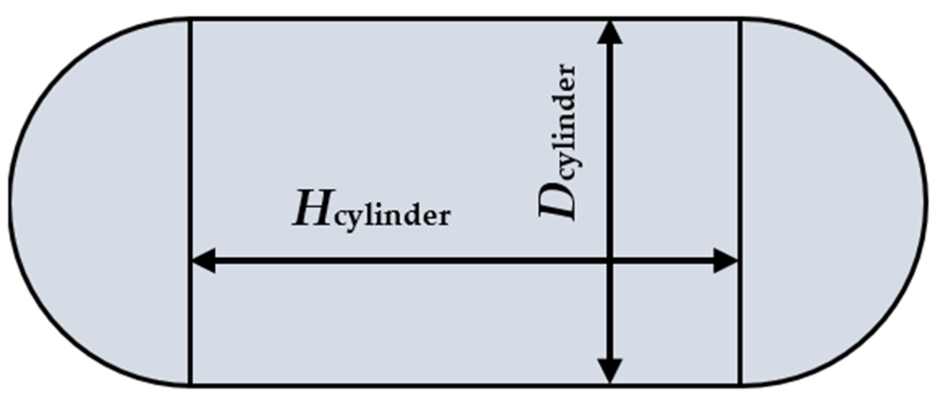
Appendix B.1. Accumulator Vessel

Figure A1 shows a schematic drawing of an accumulator vessel. It consists of a cylinder with two caps. In the simulations, it is assumed that the ratio between Hcylinder and Dcylinder is 1.5 (see accu.Hratio = 1.5 in Appendix A.1). The minimum volume of an accumulator is equal to the volume of the system between the evaporator inlet and the condenser outlet (i.e., the part of the system where vapor can occur) plus the volume of the liquid needed for expansion due to temperature variations.
The volume of the accumulator consists of the volume of the cylinder:
V cylinder = 1 4 π D cylinder 2 H cylinder ,
and the volume of the spherical caps:
V caps = 1 6 π D cylinder 3 .
From these equations, the required diameter and height of the accumulator is calculated. The wall thickness t of the cylinder and caps of the vessel are then calculated with the pressure vessel equations:
t wall ,   cylinder = p proof / burst   D cylinder 2   σ yield / ultimate   S margin ,   t wall ,   caps = p proof / burst   D cylinder 4   σ yield / ultimate   S margin ,
where pproof/burst is the proof or burst pressure for the vessel. For the wall thickness calculation for the proof pressure, the yield strength σyield of the vessel wall is used, while for the wall thickness calculation for the burst pressure, the ultimate strength σultimate is used. The factor Smargin is an additional safety margin. In the analysis, this margin is 1.25 (see accu.Smargin = 1.25 in Appendix A.1).
Figure A1. Schematic drawing of an accumulator vessel.
Energies 18 00849 g0a1

Appendix B.2. Tubing

The mass of the tubes is calculated as follows:
m tube = L tube   π d tube t wall   tube   ρ ,
where Ltube is the length of the tube, dtube is the diameter, twall is the wall thickness of the tube, and ρ is the density of the tube wall. It assumed that aluminum tubes are used, so the density is 2700 kg/m3. The thickness of the tube wall increases with the diameter. The thickness of the wall in mm is approximated as follows:
t wall   tube = d tube 60 + 0.8   mm .

Appendix B.3. Pump

The mass of the pump in kg is calculated as below:
m pump = 0.0228   Q pump + 0.3864 ,
where Q pump is the volume flow of the pump in liters/minute.

Appendix B.4. Fluid

The total fluid mass in the system is equal to the total volume of the system multiplied by the liquid density of the fluid.

Appendix B.5. Ram Air Heat Exchanger

The mass of the ram air heat exchanger consists of the mass of the aluminum fins (see “Finned air HX properties” in Appendix A.1) and plates with coolant channels. The air and fluid manifolds are not included in the mass estimation.

References

  1. Li, X.; Ye, T.; Meng, X.; He, D.; Li, L.; Song, K.; Jiang, J.; Sun, C. Advances in the Application of Sulfonated Poly(Ether Ether Ketone) (SPEEK) and Its Organic Composite Membranes for Proton Exchange Membrane Fuel Cells (PEMFCs). Polymers 2024, 16, 2840. [Google Scholar] [CrossRef] [PubMed]
  2. Shang, Z.; Hossain, M.; Wycisk, R.; Pintauro, P.N. Poly(phenylene sulfonic acid)-expanded polytetrafluoroethylene composite membrane for low relative humidity operation in hydrogen fuel cells. J. Power Sources 2022, 535, 231375. [Google Scholar] [CrossRef]
  3. Wang, Y.; Chen, K.S.; Mishler, J.; Cho, S.C.; Cordobes Adroher, X. A review of polymer electrolyte membrane fuel cells: Technology, applications, and needs on fundamental research. Appl. Energy 2011, 88, 4. [Google Scholar] [CrossRef]
  4. Revolutionising Aviation: Propelling Towards Decarbonised Skies with H2-Fuelled FC. Available online: https://brava-project.eu/ (accessed on 7 January 2025).
  5. van Es, J.; Pauw, A.; van Donk, G.; van Gerner, H.J.; Laudi, E.; He, Z.; Gargiulo, C.; Verlaat, B. AMS02 Tracker Thermal Control Cooling System commissioning and operational results. In Proceedings of the 43rd International Conference on Environmental Systems, Vail, CO, USA, 14–18 July 2013. [Google Scholar]
  6. Gorbenko, G.O.; Gakal, P.H.; Turna, R.Y.; Hodunov, A. Retrospective Review of a Two-Phase Mechanically Pumped Loop for Spacecraft Thermal Control Systems. J. Mech. Eng. 2021, 24, 27–37. [Google Scholar] [CrossRef]
  7. van Gerner, H.J.; Kunst, R.; van den Berg, T.H.; van Es, J.; Tailliez, A.; Walker, A.; Ortega, C.; Centeno, M.; Roldan, N.; Castaneda, C.; et al. Development and Testing of a Two-Phase Mechanically Pumped Loop for Active Antennae. In Proceedings of the 52nd International Conference on Environmental Systems, Calgary, AB, Canada, 12–16 July 2023. [Google Scholar]
  8. van Gerner, H.J.; de Smit, M.; van Es, J.; Migneau, M. Lightweight Two-Phase Pumped Cooling System with Aluminium Components produced with Additive Manufacturing. In Proceedings of the 49th International Conference on Environmental Systems, Boston, MA, USA, 7–11 July 2019. [Google Scholar]
  9. van Gerner, H.J.; Cao, C.; Pedroso, D.A.; te Nijenhuis, A.K.; Castro, I.; Dsouza, H. Two-phase pumped cooling system for power electronics; analyses and experimental results. In Proceedings of the 30th International Workshop on Thermal Investigations of ICs and Systems (THERMINIC), Toulouse, France, 25–27 September 2024. [Google Scholar]
  10. Tang, X.; Zhang, Y.; Xu, S. Experimental study of PEM fuel cell temperature characteristic and corresponding automated optimal temperature calibration model. Energy 2023, 283, 128456. [Google Scholar] [CrossRef]
  11. EKPO Fuel Cell Stacks. Available online: https://www.now-gmbh.de/en/projectfinder/h2sky/ (accessed on 22 October 2024).
  12. Neto, D.M.; Oliveira, M.C.; Alves, J.L.; Menezes, L.F. Numerical study on the formability of metallic bipolar plates for Proton Exchange Membrane (PEM) Fuel Cells. Metals 2019, 9, 810. [Google Scholar] [CrossRef]
  13. van Gerner, H.J.; van Benthem, R.C.; van Es, J.; Schwaller, D.; Lapensée, S. Fluid selection for space thermal control systems. In Proceedings of the 44th International Conference on Environmental Systems, Tucson, AZ, USA, 13–14 July 2014. [Google Scholar]
  14. Lemmon, E.; Huber, M.; McLinden, M. NIST Standard Reference Database 23: Reference Fluid Thermodynamic and Transport Properties-REFPROP, version 9.1; National Institute of Standards and Technology: Gaithersburg, MD, USA; Standard Reference Data Program: Gaithersburg, MD, USA, 2013. [Google Scholar]
  15. NFPA 704 Standard System for the Identification of the Hazards of Materials for Emergency Response. Available online: https://www.nfpa.org/Codes-and-Standards/All-Codes-and-Standards/List-of-Codes-and-Standards. (accessed on 18 February 2021).
  16. van Gerner, H.J.; Braaksma, N. Transient modelling of pumped two-phase cooling systems: Comparison between experiment and simulation, ICES-2016-004. In Proceedings of the 46th International Conference on Environmental Systems, Vienna, Austria, 10–14 July 2016. [Google Scholar]
  17. van Gerner, H.J.; Bolder, R.; van Es, J. Transient modelling of pumped two-phase cooling systems: Comparison between experiment and simulation with R134a, ICES-2017-037. In Proceedings of the 47th International Conference on Environmental Systems, Charleston, South Carolina, 16–20 July 2017. [Google Scholar]
  18. Donders, S.N.L.; Banine, V.Y.; Moors, J.H.J.; Verhagen, M.C.M.; Frijns, O.V.W.; van Donk, G.; van Gerner, H.J. Thermal Conditioning System for Thermal Conditioning a Part of a Lithographic Apparatus and a Thermal Conditioning Method. Patent US8610089, 2013. Available online: https://patents.google.com/patent/US8610089B2/en (accessed on 7 January 2025).
  19. Van Gerner, H.J.; Luten, T.; Scholten, S.; Mühlthaler, G.; Buntz, M.B. Test results for a novel 20 kW two-phase pumped cooling for aerospace applications. Aerospace, 2024; submitted. [Google Scholar]
  20. PFAS Ban Affects Most Refrigerant Blends. Available online: https://www.coolingpost.com/world-news/pfas-ban-affects-most-refrigerant-blends/ (accessed on 20 April 2023).
  21. ECHA, European Chemical Agency. Submitted Restrictions Under Consideration. Available online: https://echa.europa.eu/restrictions-under-consideration/-/substance-rev/72301/term (accessed on 24 January 2024).
Figure 1. Schematic drawing of a 2-PC system.
Energies 18 00849 g001
Figure 3. Figure of merit (see Equation (3)) as a function of temperature: (a) all fluids in the REFPROP database, (b) excluding flammable fluids.
Energies 18 00849 g003
Figure 4. Calculated temperatures for two-phase methanol.
Energies 18 00849 g004
Figure 5. Calculated vapor mass fraction for two-phase methanol.
Energies 18 00849 g005
Figure 6. Calculated pressures for two-phase methanol.
Energies 18 00849 g006
Figure 7. Calculated temperatures for two-phase water.
Energies 18 00849 g007
Figure 8. Calculated temperatures for liquid EGW.
Energies 18 00849 g008
Table 2. Summary table for the different fluids. The results for two phase fluids are in the blue columns, while the result for liquid EGW is in the green column.
Methanol Water Novec 649 Fluorinert 72 (C6F14) Liquid EGW
Accumulator volume 2293 L (0 L)482 L (0 L)476 L (0 L)542 L (0 L)26 L
Pump flow 463 lpm183 lpm1741 lpm1635 lpm2314 lpm
Pump power 1.6 kW0.1 kW6.6 kW4.2 kW12.9 kW
Triple point (°C) −97 °C0 °C−108 °C−86 °C~−48 °C
Mass fluid 2239 kg (38 kg)514 kg (61 kg)810 kg (260 kg)992 kg (311 kg)355 kg
Mass tubing 35 kg72 kg75 kg91 kg45 kg
Mass pump 11 kg5 kg40 kg38 kg53 kg
Mass accumulator 232 kg (0 kg)16 kg (0 kg)61 kg (0 kg)56 kg (0 kg)neglected
Mass air heat exchanger 213 kg233 kg226 kg232 kg263 kg
Total mass 2529 kg (297 kg)840 kg (372 kg)1212 kg (601 kg)1409 kg (671 kg)716 kg
2 The value between brackets is for the “no accumulator” concept.
Disclaimer/Publisher’s Note: The statements, opinions and data contained in all publications are solely those of the individual author(s) and contributor(s) and not of MDPI and/or the editor(s). MDPI and/or the editor(s) disclaim responsibility for any injury to people or property resulting from any ideas, methods, instructions or products referred to in the content.

