Abstract
Due to the complex mechanical structure of the spring-operated mechanism, its failure mechanisms often exhibit a multi-faceted nature, involving various potential failure sources. Therefore, conducting a failure mechanism analysis for multi-source faults in such systems is essential. This study focuses on the design of composite faults in combination operating mechanisms and develops simulation scenarios with varying levels of fault severity. Given the challenges of traditional simulation methods in performing quantitative analysis of core jamming faults and the susceptibility of the core’s motion trajectory to external interference, this paper innovatively installs a spring-damping device at the extended core position. This ensures that, during the simulation of core jamming faults, the motion trajectory remains stable and unaffected by external factors, while also enabling precise control over the degree of jamming. As a result, the simulation more accurately reflects real fault conditions, thereby enhancing the accuracy and practicality of diagnostic model outcomes. This study employs the Morlet wavelet transform to convert the current and displacement signals in the time series into time-frequency spectrograms. These spectrograms are then processed using the ResNet50 deep residual neural network for feature extraction and fault classification. The results demonstrate that, when addressing the diagnostic problem of small-sample data for operating mechanism faults, ResNet50, with its residual structure design, exhibits significant advantages. The convolutional layer strategy, which first performs dimensionality reduction followed by dimensionality expansion, combined with the use of the ReLU activation function, contributes to superior performance. This approach achieves a fault recognition accuracy of up to 91.67%.
1. Introduction
Circuit breaker operating mechanisms, when subjected to long-term mechanical stress and environmental influences, inevitably exhibit various mechanical damages or defects over time [1]. Operational surveys of high-voltage circuit breaker mechanisms indicate that mechanical defects in the operating mechanism account for 63.8% of the instances of breaker refusal to operate, representing a major contributing factor [2]. The causes of these faults are complex and involve a combination of factors, including the jamming of the opening and closing coil core, significant motion resistance encountered during the core’s accelerated movement, as well as physical damage or structural deformation of the coil and related transmission components.
It has been reported that in a 110 kV substation in Liaoning Province, the CD10 model operating mechanism experienced multiple atypical operational incidents within its one-year service period. These incidents were primarily characterized by delayed closing actions and failure of the opening function. Upon thorough investigation, it was confirmed that the fault was caused by a combination of issues, including jamming of the opening and closing coil core, deviation of the actuator rod stroke from the normal range, excessive setting of the limit screw, and twisting deformation of the linkage in the transmission mechanism [3]. Due to the complexity of its mechanical structure, the fault mechanism is often associated with multiple potential failure sources. Therefore, a comprehensive investigation into the failure mechanisms of multi-factor faults in such systems is an indispensable task [4].
Researchers both domestically and internationally have proposed various signal processing methods in previous studies, generally divided into two stages: signal feature extraction and fault classification. Traditional methods, such as modal analysis [5], feature entropy [6], wavelet thresholding [7], and frequency response function estimation [8], have been widely applied in the field of signal feature extraction. Reference [9] applied the Relief algorithm for dimensionality reduction and optimization of the current characteristics of the opening and closing coils, followed by fault classification using a self-organizing map (SOM) network. Reference [10] established characteristic curves for the current waveforms in the opening and closing coils to explore their correlation with the performance of the electromagnetic and mechanical transmission systems. Fault diagnosis and evaluation were precisely carried out through magnetic circuit analysis. Reference [11] integrated coil current signals with additional signal processing techniques to construct a feature vector space and then used support vector machine (SVM) techniques to distinguish between fault types. However, the aforementioned studies mainly focus on identifying single mechanical fault states, and there is a lack of in-depth exploration and systematic research on the dynamic characteristics of operating mechanisms under complex fault conditions, where multiple concurrent or interacting defects are present.
Given the high requirements for data accuracy and completeness in diagnostic models, improper data processing methods inevitably lead to deviations in diagnostic results. To address this issue, researchers both domestically and internationally have increasingly integrated artificial intelligence into equipment fault diagnosis models. Reference [12] extracts the energy distribution features of signal subspaces using wavelet transforms and builds an auto-encoding deep fault diagnosis model through distributed training and labeled fine-tuning. Reference [13] combines the LVQ neural network and DAG-SVM to input zero-point fault current parameters for deep learning, detecting corresponding fault types. However, due to the limited selection of feature parameters and the scarcity of signal resources, the current models face limitations such as high training loss errors and a lack of information correlation. Additionally, methods like radial basis function (RBF) neural networks [14], backpropagation (BP) neural networks [15], support vector machines (SVM) [16], and decision trees [17,18] all belong to the category of traditional shallow learning architectures. Given the instantaneous nature of operating mechanism actions, the complexity of signal transmission paths, and the diversity of external interference factors, these shallow network techniques are often prone to the “curse of dimensionality”. This leads to excessively high complexity in the feature space and faces challenges such as the model becoming trapped in local optima and poor generalization performance [19,20].
To address the aforementioned limitations, this study first redefines the classification of faults and their severity levels, designing a series of composite fault scenarios to comprehensively cover the various defect combinations that an operating mechanism may encounter. To accurately capture the dynamic behavior of the operating mechanism under different operating conditions, an efficient current and displacement signal acquisition system platform was developed. Using the Morlet wavelet analysis strategy, time-series signals are transformed into time-frequency images, which serve as feature vectors for subsequent analysis. This approach enhances the temporal and spatial representation capabilities of the features.
The proposed ResNet50-based fault diagnosis method for spring operating mechanisms demonstrates novelty and contributions in the following aspects. Firstly, the deep architecture with residual connections addresses the vanishing gradient problem during deep network training, thereby enhancing the model’s learning capability and robustness. Comparative experimental results indicate that ResNet50 outperforms other deep learning models (e.g., MobileNetV2 and Transformer) in handling complex small-sample datasets.
The model effectively addresses the difficulties of training deep networks through its residual connection mechanism, ensuring the efficient propagation of gradients, thereby enhancing the model’s performance in handling composite mechanical fault identification tasks. The study uses the CT-26 spring-operated mechanism as the experimental subject, applying the proposed diagnostic model for comprehensive evaluation. The goal is to verify the model’s ability and effectiveness in accurately identifying composite mechanical faults in real-world scenarios, providing a scientific foundation and technical support for health management and fault prediction in high-voltage circuit breakers.
2. Simulation Design of Mechanical Faults in the Spring-Operated Mechanism
In this study, we conducted simulated designs for three types of faults—abnormal core gap, coil core sticking, and abnormal core stroke—in the CT-26 spring operating mechanism produced by Taikai High Voltage Switch Co., Ltd. in Shandong, China, under its brand-new condition. The specific design schemes are as follows.
2.1. Design for the Abnormal Core Gap Fault
The core gap distance T quantifies the vertical distance between the top of the coil core (A) and the bottom of the opening lever (B). The specific value of T is precisely controlled by adjusting the nut c. After multiple operations of opening and closing the spring-operated mechanism under dynamic conditions, the accelerated movement of the core collides with the lever, generating an opposing force that causes the positioning nut c to loosen. This loosening effect directly leads to an undesirable increase in the core gap T, thereby increasing the risk of failure when executing the opening command. Based on extensive measurements of core gap values under healthy conditions and discussions with technical production experts, the standard range for T is determined to be between 0.8 mm and 1.2 mm.
As shown in Figure 1, the core gap distance T is controlled by the core adjustment bolt C. Rotating bolt C to the left reduces the gap distance, while rotating it in the opposite direction increases the gap. With repeated opening and closing commands issued to the coil, the opposing surfaces of A and B experience continuous collisions over time. During these impacts, the forces and reaction forces cause bolt C to loosen, leading to an enlargement of the core gap.
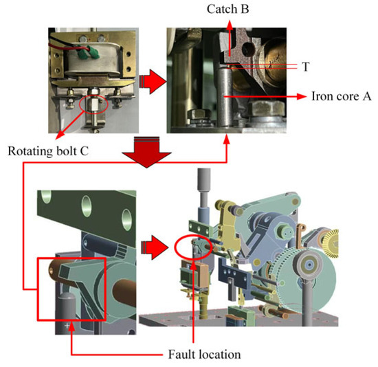
Figure 1.
Simulation of core gap fault.
Figure 1 illustrates the simulation of the core gap fault. By adjusting the rotation angle of bolt C, the distance T between A and B is made greater than the upper limit of the enterprise’s standard, 1.2 mm. The red box in the figure indicates the fault location, which is at the position where the limit lever meets the core. To investigate the operational status of the mechanism under different fault severities, the experiment designs core gap values of 1.6 mm (Level 1 gap anomaly) and 2.0 mm (Level 2 gap anomaly).
Coil Core A: Refers to the part of the actuating mechanism responsible for driving the trip action of the circuit breaker.
Trip Lever B: A component of the mechanical structure that is responsible for locking and releasing the trip action.
Core Gap T: Refers to the vertical distance from the top of Coil Core A to the bottom of Trip Lever B.
Adjustment Mechanism: (1) The component C nut is a mechanical component used to precisely adjust the core gap distance (T). By rotating or shifting the nut, the distance between the coil core and the trip lever can be fine-tuned to ensure optimal operational performance. (2) The standard range for T was determined to be between 0.8 mm and 1.2 mm. This was based on extensive measurements of core gaps in healthy states, followed by discussions with technical and production experts.
2.2. Design of Core Jamming Fault
The core, as the key component of the operating mechanism’s coil, is responsible for receiving and responding to the coil’s action commands. When the coil is energized, the electromagnetic attraction acts on the core, causing it to overcome its own resistance and accelerate in motion, ultimately colliding with the upper limit lever to achieve the opening and closing functions of the mechanism. However, mechanical wear over long-term operation can cause the surface of the core to become rough. Additionally, prolonged exposure to a humid environment or lack of anti-rust oil protection can lead to core corrosion. Under the combined effects of these unfavorable factors, the motion resistance of the core increases, necessitating a higher coil current to enhance the electromagnetic attraction in order to ensure the proper operation of the mechanism.
In previous studies, various methods have been used to simulate core jamming, including suspending weights and introducing materials such as foam or wood shavings into the core gap. However, suspending weights can cause excessive oscillation of the core’s motion, resulting in unstable force simulation during movement. On the other hand, introducing foam, wood shavings, or similar materials makes it difficult to quantify the degree of jamming, leading to rough data and limited practical engineering guidance.
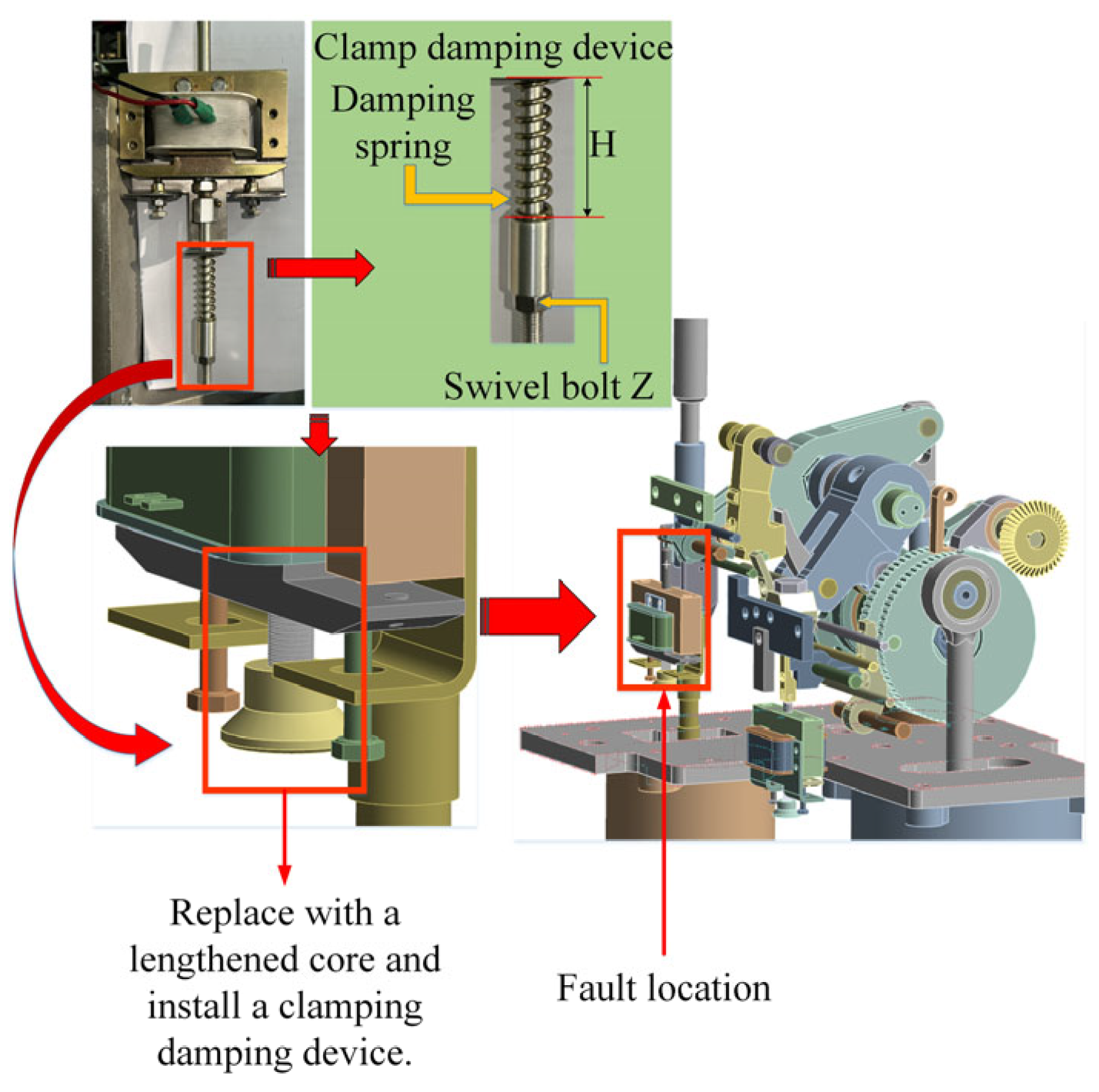
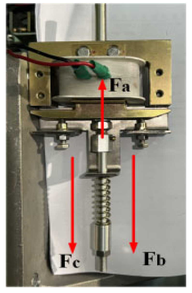
To address the aforementioned issues, this study introduces the use of a damping device to simulate core jamming. The overall fault simulation design is shown in Figure 2. The original core in the coil is replaced with an elongated core that has threads at the bottom, maintaining the same operational state as the original core. A jamming damping device is installed in the middle of the elongated core. The damping device consists of a damping spring and a rotating bolt Z, which is used to adjust the force of the damping spring. During the upward motion of the core, the damping spring is automatically compressed, successfully simulating the core jamming fault. The force state of the core at this point is shown in Figure 3. The electromagnetic attraction force Fa must overcome both the core’s own resistance Fb and the externally applied damping force Fc.

Figure 2.
Simulation of iron core jamming fault.

Figure 3.
Force state of iron core jamming.
To specifically diagnose the severity of core jamming in the operating mechanism, two different fault severities are set. In Figure 2, the length H of the damping spring represents the severity of the jamming. The unstretched length of the damping spring is 5 cm. In the experiment, the spring length H is set to 4.6 cm (Level 1 core jamming) and 4.2 cm (Level 2 core jamming) for the two fault severity levels.
During the operation of the spring actuation mechanism, the core moves upward or downward during the opening or closing process. In this design, the core compresses the damping spring during its upward movement, simulating the core binding fault. The process is as follows:
Core Moving Upward: When the electromagnetic force acts on the core, the core begins to move upward. During this motion, the damping spring is gradually compressed, generating an opposing resistance.
Force Analysis: During the upward motion of the core, three main forces are at play—(1) electromagnetic attraction, which is the primary force driving the upward motion of the core, (2) the core’s own resistance, which includes the core’s weight and internal friction, and (3) additional externally applied damping resistance, which is provided by the damping spring, simulating the frictional force encountered when the core binds.
During the upward movement, the core must overcome these resistances to complete the operation. By adjusting the position of the rotating bolt Z, the pre-tension of the damping spring can be altered, thereby regulating the total resistance the core experiences.
2.3. Coil Stroke Fault Design
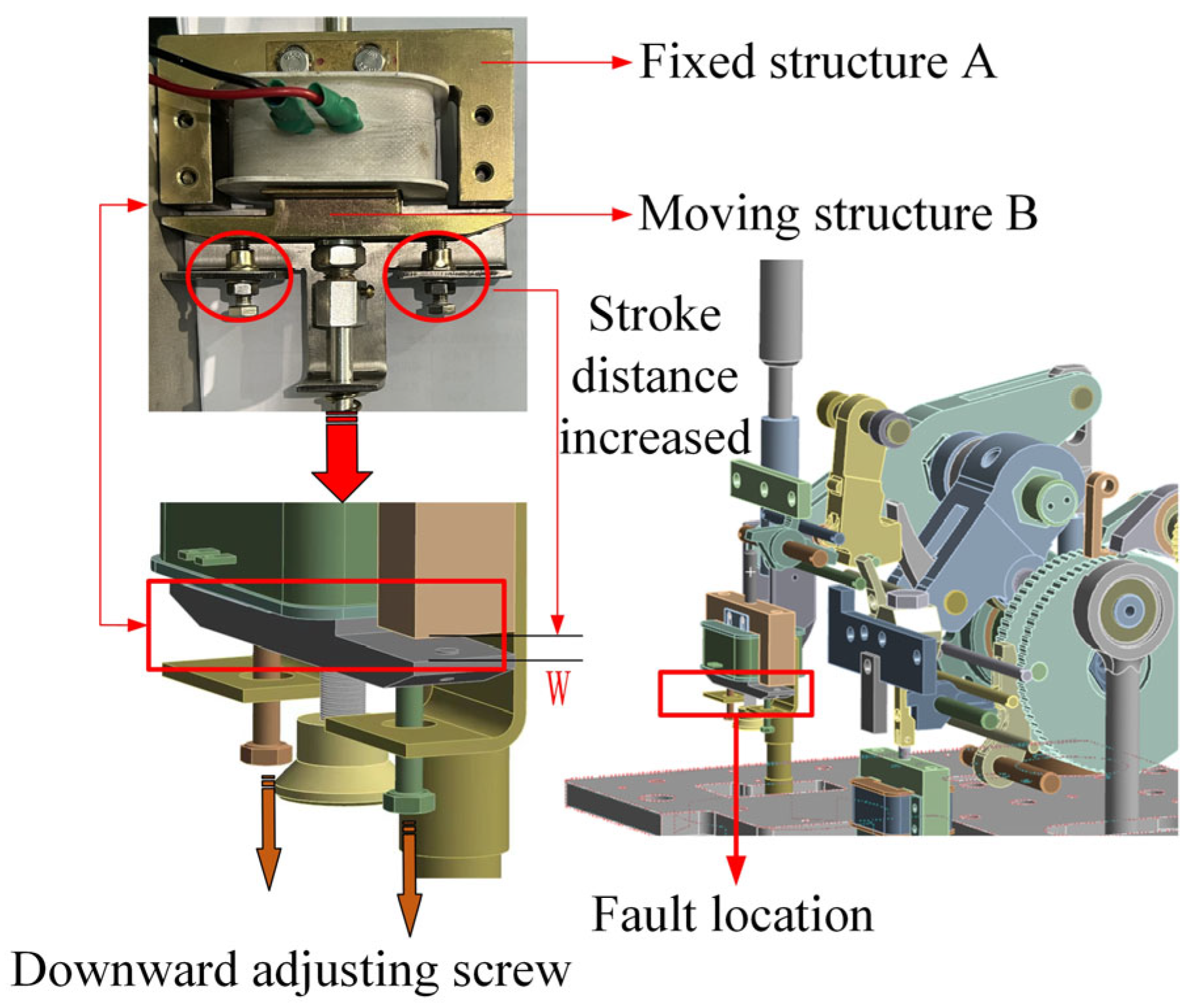
The overall structure of the opening and closing coil consists of four parts: the fixed structure A, the moving structure B, the coil, and the core. As shown in Figure 4, the distance W between the fixed structure A and the moving structure B is referred to as the core stroke distance. The coil core and structure B form a unified assembly. To maintain the stability of the core’s movement and mitigate oscillation and swaying during motion, a damping spring is placed between structures A and B.

Figure 4.
Simulation of abnormal stroke distance fault.
In Figure 4, the constraint bolts at both ends of Structure B, marked by the red circles, are used to precisely adjust the stroke distance W by rotating the bolts. This adjustment mechanism ensures that the actuator remains in optimal working condition during the open/close operations. The technical details are as follows:
- (1)
- Structure and Adjustment Mechanism
Fixed Structure A: This component limits the maximum movement range of the core, ensuring that the core does not exceed the predetermined range under the influence of electromagnetic forces.
Structure B and Constraint Bolts: Structure B consists of two key components—the core and the constraint bolts. By rotating the constraint bolts, their preload force can be adjusted, thus controlling the stroke distance W. The design of the constraint bolts allows for precise control of the core’s travel to meet different operational requirements.
- (2)
- Mechanical Analysis During Operation
Electromagnetic Force: When the coil is energized, a strong electromagnetic field is generated, providing an upward electromagnetic force to the core. This force drives the core to overcome gravity and other resistances, completing the open/close operation.
Stroke Distance W: This is defined as the distance from the core’s initial position to the maximum displacement point. By adjusting the angle of the constraint bolts, this distance can be precisely controlled, ensuring it stays within the specified range (3.9 mm to 4.3 mm).
- (3)
- Industry Standards and Experimental Setup
According to industry standards, the stroke distance W should be strictly controlled within the range of 3.9 mm to 4.3 mm. To investigate the impact of excessive stroke on the actuator’s performance, two abnormal stroke distances were designed for experimental verification:
First-Level Stroke Abnormality: Set the stroke distance W = 4.9 mm to simulate a slight overtravel condition.
Second-Level Stroke Abnormality: Set the stroke distance W = 5.9 mm to simulate a more severe overtravel condition.
3. Design of Composite Faults in the Operating Mechanism and Experimental Data Acquisition System
In the actual operating environment of the mechanism, due to continuous mechanical loads and environmental interactions, the internal components often undergo comprehensive aging and performance degradation. This degradation does not occur in isolation but exhibits the characteristic of multiple simultaneous faults. Previous research has largely been confined to signal feature acquisition and analysis under single fault modes, with isolated exploration of the operational characteristics of the mechanism under each fault condition. This approach overlooks the interactions and superposition effects between faults. Compared to the complex real-world situations, it presents certain simplifications and deviations, failing to adequately reflect the true dynamic behavior and potential fault evolution paths of the operating mechanism when facing multiple simultaneous faults. Therefore, research on fault diagnosis of operating mechanisms urgently requires a more comprehensive approach that is closer to actual working conditions to accurately identify and assess the system’s state under multi-fault coexistence.
3.1. Composite Fault Design
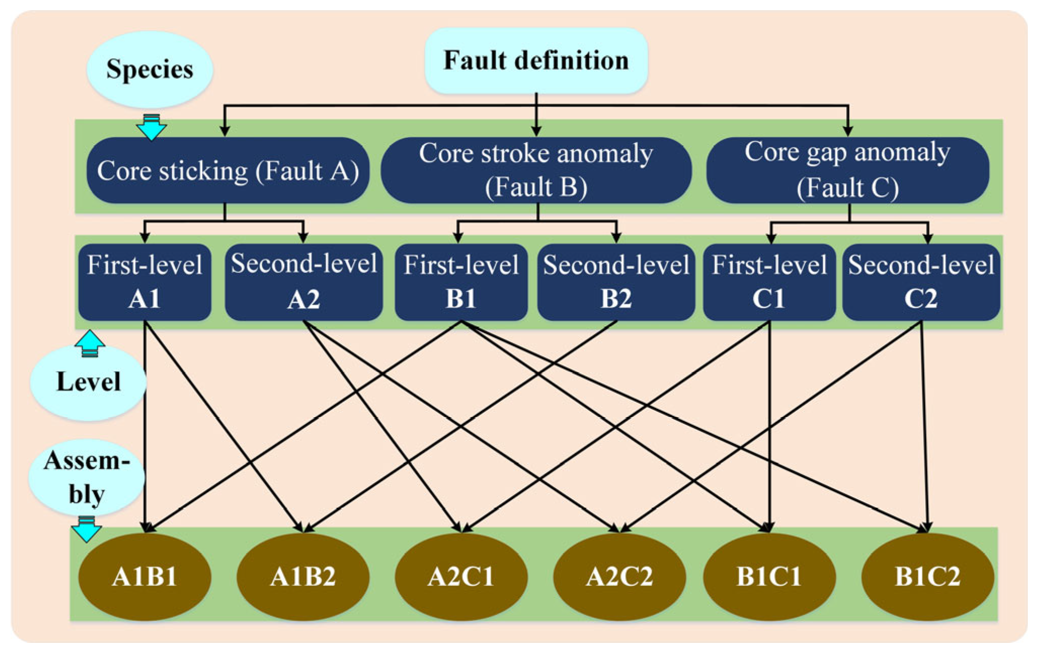
This study combines single faults of varying severities to design six types of composite faults. The specific design is shown in Figure 5.
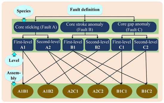
Figure 5.
Combination Fault Definition Diagram.
In Section 2 of this paper, the faults related to the core sticking, core stroke anomaly, and core gap anomaly are named as Fault A, Fault B, and Fault C, respectively. Specifically, in the case of core sticking, the first-level sticking (spring length H set to 4.6 cm) is designated as Fault A1, and the second-level sticking (spring length H set to 4.2 cm) is designated as Fault A2. In the case of core stroke anomaly, the first-level anomaly (stroke distance 4.9 cm) is designated as Fault B1, and the second-level anomaly (stroke distance 5.9 cm) is designated as Fault B2. In the case of core gap anomaly, the first-level gap distance (1.6 mm) is designated as Fault C1, and the second-level gap distance (2.0 mm) is designated as Fault C2.
The overall composite faults are categorized into three types, with each category consisting of two levels of severity. These different fault types are selectively combined in pairs of varying degrees. As shown in Figure 5, the composite faults are as follows: first-level core sticking and first-level stroke anomaly (A1B1), first-level core sticking and second-level stroke anomaly (A1B2), second-level core sticking and first-level gap anomaly (A2C1), second-level core sticking and second-level gap anomaly (A2C2), first-level stroke anomaly and first-level gap anomaly (B1C1), and first-level stroke anomaly and second-level gap anomaly (B1C2). These represent a total of six abnormal operating conditions.
3.2. Design of the Composite Fault Acquisition System for the Actuating Mechanism
As shown in Figure 6, the rotational sensor is positioned at the output shaft side of the actuating mechanism. The output end of the sensor is connected to the input terminal of the switch characteristic tester. The tester converts the rotational angle of the output shaft into the displacement distance of the moving contact through an analog-to-digital conversion. The sequential displacement data are then stored in the test record.
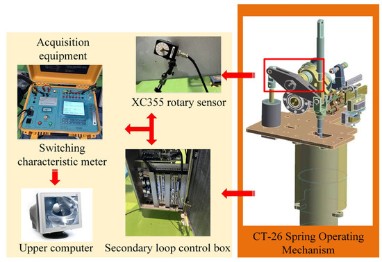
Figure 6.
Experimental collection system.
The experimental setup was configured as follows: The breaker’s split-off and closing circuits in the actuating mechanism’s secondary control loop were connected to the yellow and red ports of the high-voltage switch characteristic tester, with the black port designated as the common terminal. A 220 V power supply was utilized to energize the energy storage circuit. Three-phase contact circuits (A, B, and C) of the circuit breaker were interfaced with the tester’s output ports (yellow, green, and red). Voltage regulation was controlled by the characteristic tester, which was configured with a sampling time of 150 ms.
For data acquisition, a circuit breaker switch characteristic tester was employed, featuring six contact status indicators for state verification and wiring validation. The instrument’s specifications included a time measurement range of 1–20,000 ms (±(0.005%t + 0.1) ms accuracy), analog input range of 0–5 V, and coil current measurement capability of 0–2/20 A with 10 mA resolution for both DC and AC measurements. Displacement signals from the circuit breaker’s dynamic and static contacts were captured using an XC-355 rotary sensor, characterized by 16-bit resolution, ±0.005° accuracy, 9–36 V operating voltage, and 2500 mm effective measuring stroke.
4. Signal Preprocessing and Morlet Wavelet Transform Under Fault Conditions
In this experiment, a detailed fault simulation and data collection were conducted on the opening and closing processes of the actuator using the signal acquisition system shown in Figure 6. The switch characteristic tester was used to control the actuator’s operation. Independent experimental trials were carried out for six different types of combined faults, with 50 sets of current and displacement signal samples collected for each fault type. In total, 600 sets of valid data were acquired.
Considering that the raw current signals are inevitably influenced by various external interference factors during the data collection phase, a five-point cubic smoothing technique was applied for data preprocessing to filter out irregular fluctuations and background noise. To further explore the intrinsic features of the signals, wavelet transform analysis was employed. The current and displacement signals, processed through both smoothing and wavelet transform, were then used as input data for the convolutional neural network (CNN) model.
4.1. Five-Point Cubic Smoothing of Current Signals
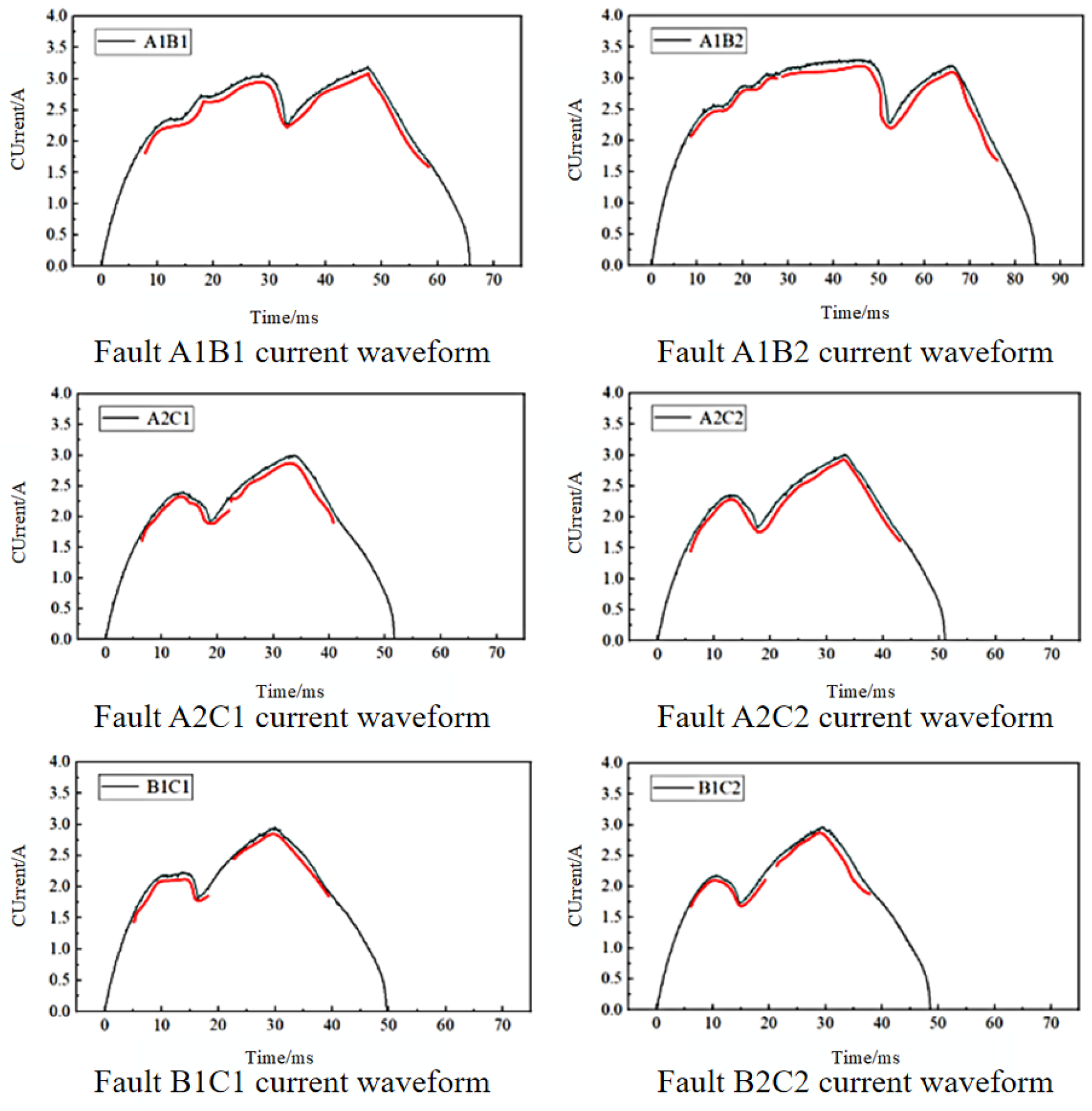
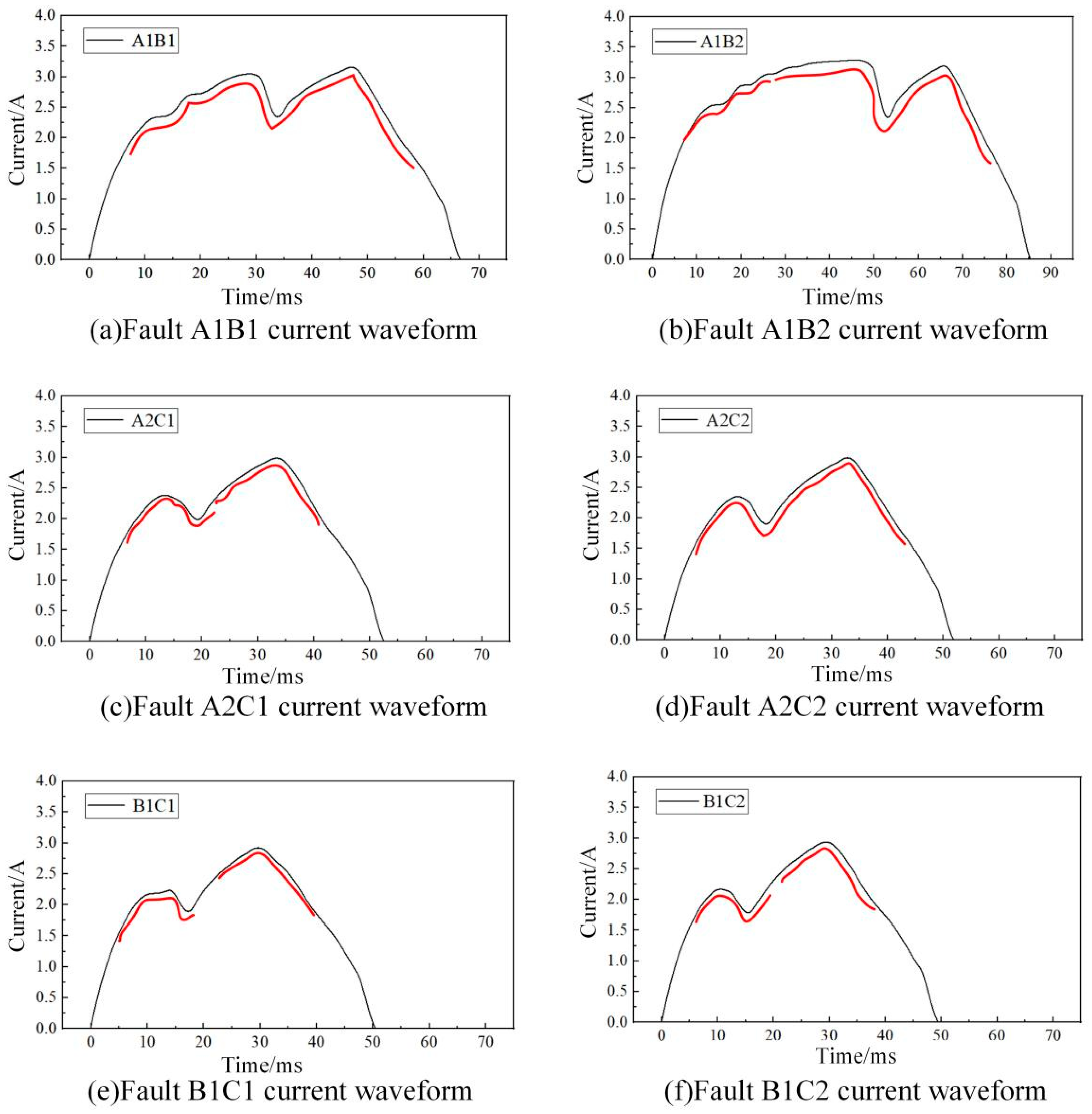
Figure 7 illustrates the variation of the current signal in the coil of the actuator under the six predefined composite fault modes. The red-marked areas highlight the noise and spikes in the current signal. These disturbances are primarily caused by factors such as magnetic field coupling effects, electromagnetic radiation interference, and leakage coupling, among others. The characteristics of such interference signals are manifested by their high-frequency components and periodic appearance patterns. These features significantly disrupt the time-frequency spectrum distribution during the wavelet transform of the original current signal, reducing the accuracy and reliability of signal analysis.
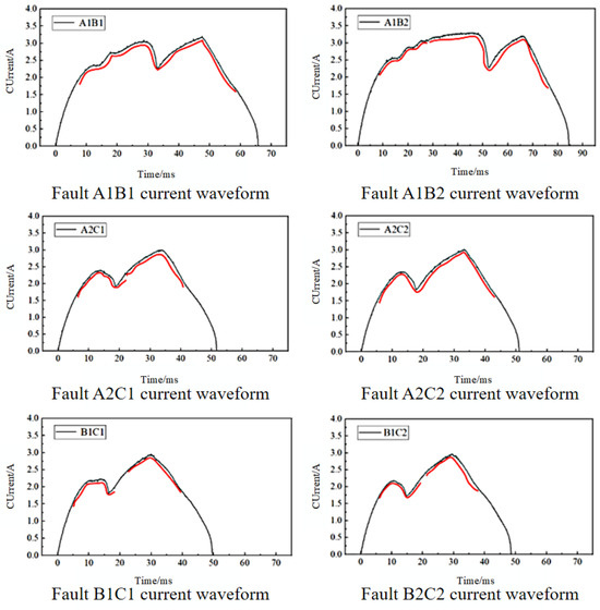
Figure 7.
Waveforms of six combinations of fault currents.
This study employs the five-point cubic spline smoothing method, constructing a local cubic polynomial curve with five points to fit the original data. This approach effectively mitigates high-frequency noise interference while preserving the overall shape of the signal. It ensures that the signal is more focused on the true characteristics of the current signal, thereby improving the accuracy and effectiveness of fault diagnosis.
To divide the original current waveform into n evenly spaced points, the current waveform data can be represented as X0 < X1 < X2 < … < Xn−1. For each interval between two adjacent points, the cubic polynomial is applied, considering the two neighboring points before and after each data point. The cubic polynomial is given as follows:
The coefficients a0, a1, a2, a3 are determined using the least squares method, and the five-point cubic smoothing formula is obtained as follows:
The fundamental principle of the five-point cubic smoothing method is that the number of data points for the curve is greater than five, where represents the improved value of . Since the sampling data points for the coil current are much greater than five, to ensure symmetry in the smoothing effect, the endpoints of the sampled data are calculated using, , , , and , while the midpoint interval points are computed using . The denoised and smoothed coil current waveform is shown in Figure 8.
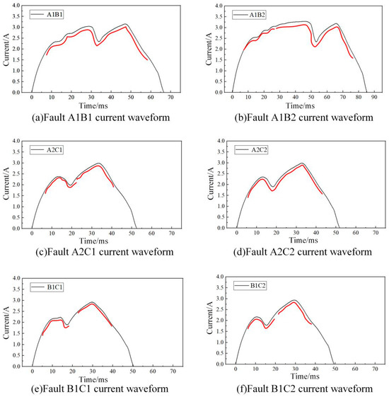
Figure 8.
Current waveform after combined fault smoothing.
4.2. Time Domain Waveform of Displacement Signal
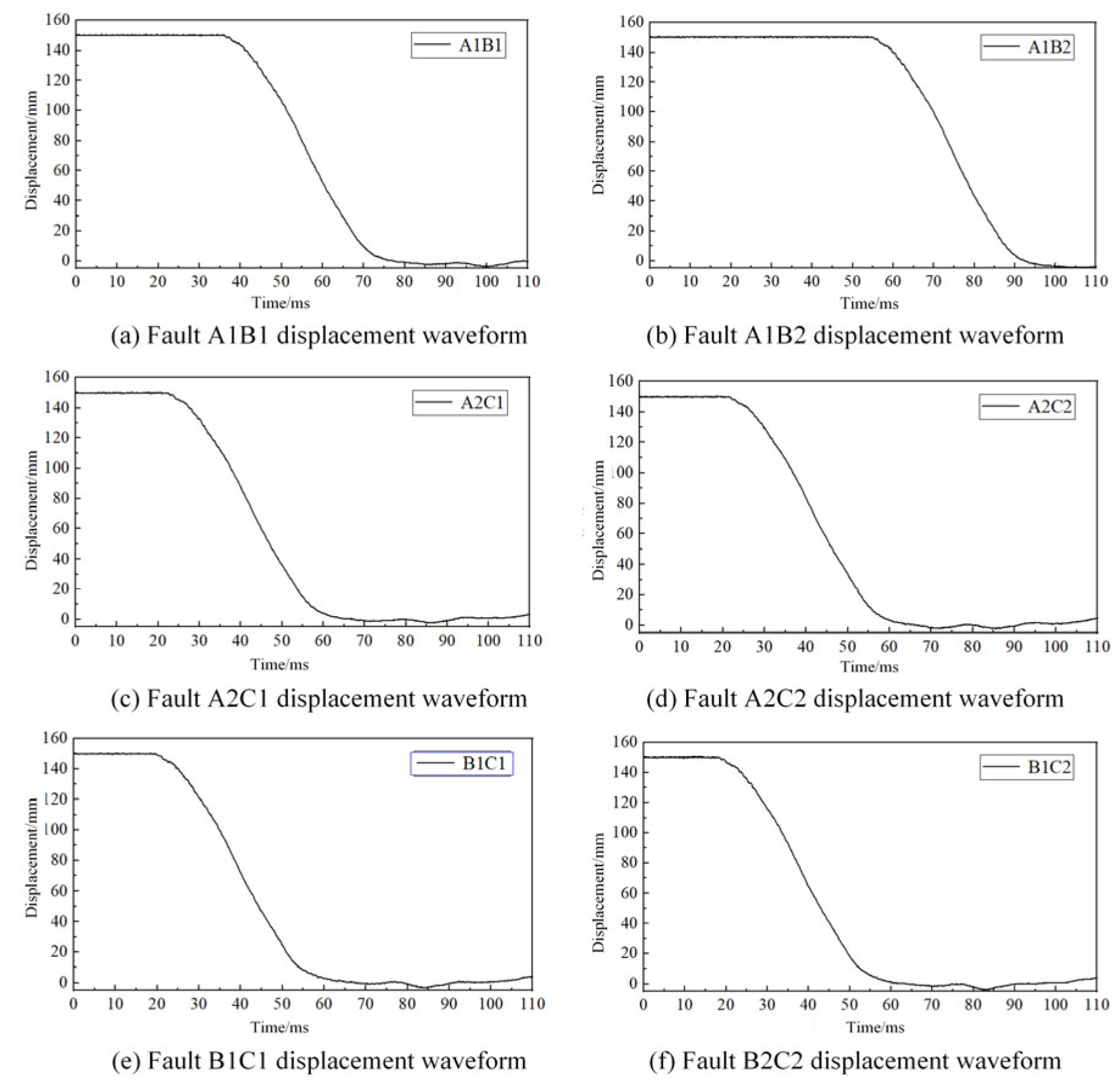
Compared to the coil current signal, which may be subject to multiple interferences, these disturbances are significantly suppressed or eliminated in displacement measurements. As a result, the acquired displacement signal exhibits high smoothness and low noise levels, making it suitable for direct frequency-domain transformation analysis. Figure 9 presents the displacement variation curve during the separation operation of the moving contact under six different combination fault scenarios.
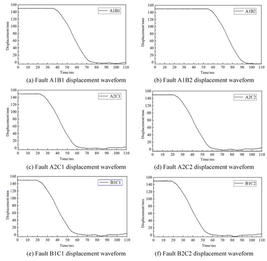
Figure 9.
Combination fault contact displacement waveform.
4.3. Time-Domain Signal Feature Representation via Morlet Wavelet Transform
Traditional Fourier transform, a tool for frequency-domain analysis, decomposes a signal into a linear combination of sinusoidal and cosine basis functions, effectively revealing its spectral composition and providing valuable insights into the signal’s frequency structure. However, it assumes that the signal is stationary throughout the observation period, meaning its statistical properties remain constant over time. This assumption limits the applicability of Fourier transform when analyzing non-stationary signals with time-varying characteristics. In particular, Fourier transform struggles with time localization and local feature analysis due to its fixed global time window, which cannot adapt to the dynamic variations of the signal across different time scales.
Wavelet transform, with its time-frequency adaptive characteristics, utilizes basis functions (wavelets) that not only provide multi-resolution properties in the frequency domain but also allow for scaling and translation in the time domain. The wavelet basis can offer finer time resolution in the high-frequency regions (rapidly varying parts of the signal) and broader frequency resolution in the low-frequency regions (slowly varying trends). By dynamically adjusting the width of the analysis window according to the signal’s characteristics, it localizes the signal in the time domain while maintaining good resolution in the frequency domain, effectively capturing and analyzing the local time-frequency features of the signal. This overcomes the fixed time window limitation of the traditional Fourier transform, significantly enhancing the local analysis capability of the signal.
To obtain the frequency-domain features of the coil current and contact displacement under different fault conditions, this study employs the Morlet wavelet analysis method to transform the two-dimensional time-domain signals into time-frequency spectrograms. This facilitates the extraction of various signal features from the spectrogram, allowing for a multi-dimensional representation of the signal characteristics of the actuator under multiple combined mechanical faults. The wavelet basis function is a single-frequency complex sinusoidal function with a Gaussian envelope, as shown in Equation (3).
The wavelet basis function is obtained by scaling and translating, as shown in Equation (4).
Within the framework of wavelet analysis, parameter a serves as a scaling factor that adjusts the size of the observation window, directly influencing the degree of stretching or refinement in signal analysis. Increasing the value of a reduces the center frequency of the complex trigonometric function, slows the exponential decay process, and extends the support region of the Gaussian function. The direct consequence of this change is a reduction in the bandwidth of the wavelet in the frequency domain, which enhances the resolution of spectral analysis, allowing for a more detailed and differentiated representation of the signal’s time-frequency characteristics. Parameter b controls the translation of the wavelet basis function in the time domain, providing a tool for time localization in signal analysis. This enables feature extraction not only in the frequency domain but also with precise time localization in the time domain.
Figure 10 illustrates the time-frequency representation of the signal after wavelet transformation, providing a clear depiction of how the signal’s energy distribution varies with time and frequency. Each time-frequency feature point represents the intensity or activity level of the original signal at a specific moment and frequency, offering valuable time-frequency information. This representation aids in gaining a deeper understanding of the signal structure, identifying potential patterns, and supporting applications such as fault detection.
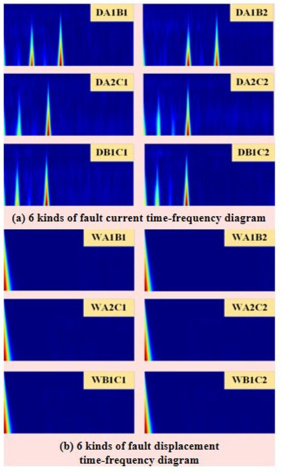
Figure 10.
Time frequency map after Moret wavelet transform.
5. Combined Mechanical Fault Diagnosis with ResNet50
In this study, the time-frequency spectrograms of current and displacement under six types of combined faults are used as input data for model training. However, traditional neural networks typically require large datasets for training and model optimization. When the model is overly complex and the training data are limited, overfitting may occur, leading to poor generalization and suboptimal performance on test data. As the network depth increases, the overall performance of the model may deteriorate rather than improve. This study integrates the ResNet50 diagnostic model and compares it with three other models: MobileNetV2, Transformer, and Vision Transformer. The specific technical roadmap is shown in Figure 11.
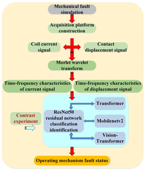
Figure 11.
Roadmap of fault diagnosis technology for operating mechanisms.
5.1. Feature Extraction with ResNet50 Model
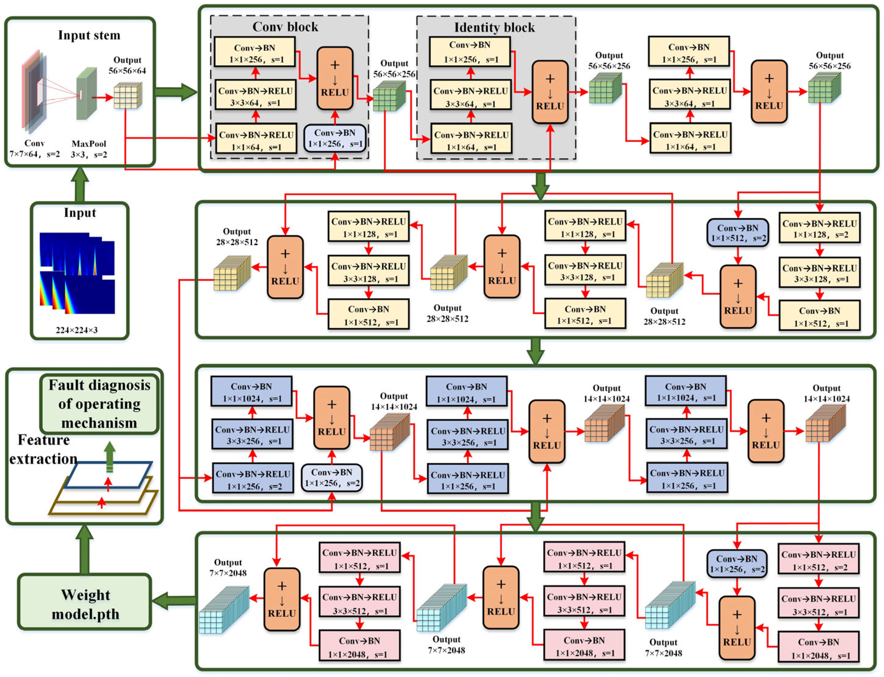
The ResNet50 deep residual network excels in capturing time-frequency image features from the actuator fault states by applying deep convolution on time-frequency spectrogram datasets. Its core advantage lies in the introduction of residual blocks, which effectively address the vanishing gradient and representation bottleneck issues commonly found in deep neural networks. This design enables the network to learn from the original features at deeper layers, making it highly adaptable to various image recognition tasks. As a result, it significantly enhances the accuracy of actuator image recognition. The overall structure of the model is shown in Figure 12.
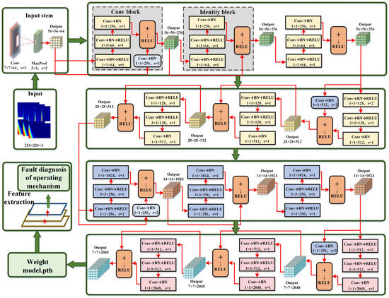
Figure 12.
Overall structure of the algorithm in this article.
To address the issue of insufficient samples, various data augmentation techniques were employed in this study, including random cropping, rotation, and flipping, to generate more diverse training samples. Regarding the dataset imbalance problem, the SMOTE resampling technique and a modified loss function were implemented to ensure optimal model performance on minority classes.
The overall structure of the ResNet50 algorithm consists of two basic building blocks: the Conv-block and the Identity-block. The Conv-block, also known as the convolutional block, is composed of several convolutional layers designed to extract and recognize key information from the actuator images. The typical structure of a Conv-block includes three parts: the 1 × 1 convolutional layer, which reduces the number of channels in the actuator image, the 3 × 3 convolutional layer for feature extraction, and another 1 × 1 convolutional layer to maintain dimensionality and restore the original number of channels. Conv-blocks are typically placed at the input stage to learn low-level features from the time-frequency images of the actuator.
The Identity-block, based on identity mapping, is also composed of three convolutional layers, and its structure is similar to that of the Conv-block. The 1 × 1 convolutional layer is used to maintain or reduce the number of channels, while the 3 × 3 convolutional layer is used for feature extraction. The final 1 × 1 convolutional layer restores the number of channels. The Identity-block maintains consistent input and output dimensions, and the feature information from the input is directly added to the output through a skip connection. This mechanism effectively addresses the issues of vanishing and exploding gradients typically encountered in deeper networks.
5.2. Model Fault Diagnosis Results and Comparative Experiments
5.2.1. Model Development Environment and Dataset Preparation
The model was built using the PyTorch 1.8.0 framework. In the experiments, the number of training epochs was set to 200, weight decay was set to 0.0005, and the learning rate was adjusted within the range of 0.01 to 0.0001. The stochastic gradient descent (SGD) optimizer was employed. The dataset was divided into two categories: current and displacement datasets. For each of the six fault combinations, the current dataset (denoted by the symbol ‘D’) and the displacement dataset (denoted by the symbol ‘W’) were created. Each dataset was split in a 4:1 ratio, with 40 samples used for training and 10 samples for testing, resulting in a total of 600 images across both datasets.
5.2.2. Comparison of Fault Diagnosis Model Performance for Actuating Mechanism
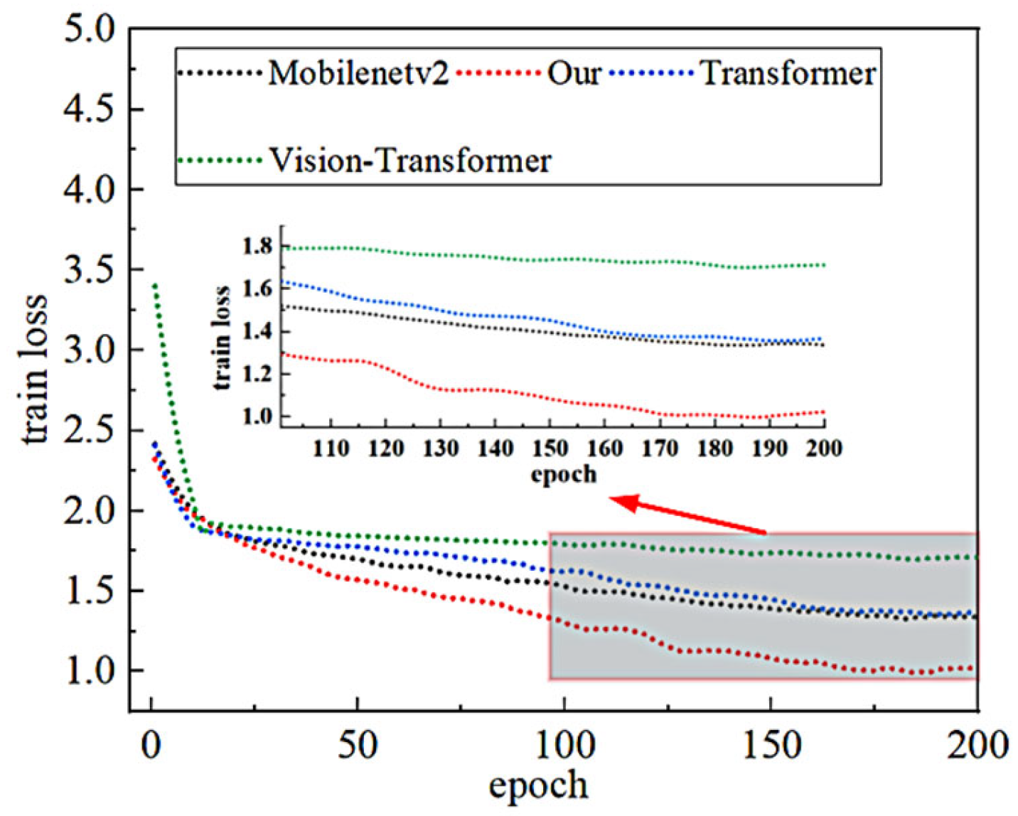
This study compares the performance of the ResNet50 model in diagnosing small-sample faults in the spring-actuating mechanism with three other models: MobileNetV2, Transformer, and Vision Transformer. The loss function for each model is shown in Figure 13.
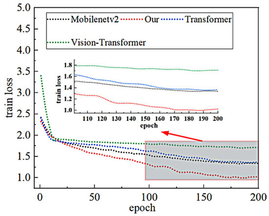
Figure 13.
Loss function value transformation curve.
The loss function provides a quantitative method to evaluate the discrepancy between the model’s predictions and the actual observed values. By minimizing the value of the loss function, the model parameters are optimized to improve prediction accuracy, prevent overfitting, and introduce regularization terms to balance model complexity and predictive capability.
As shown in Figure 13, after the 100th training epoch, the training loss of the V-T diagnostic model converges at 1.8. The Transformer and MobileNetV2 models exhibit better training loss, converging at 1.4. All three models have a loss greater than 1. However, when applied to small-sample data classification, ResNet50 shows a significant improvement, with the loss converging to 0.85 after the 170th epoch, demonstrating a notable enhancement in model learning performance.
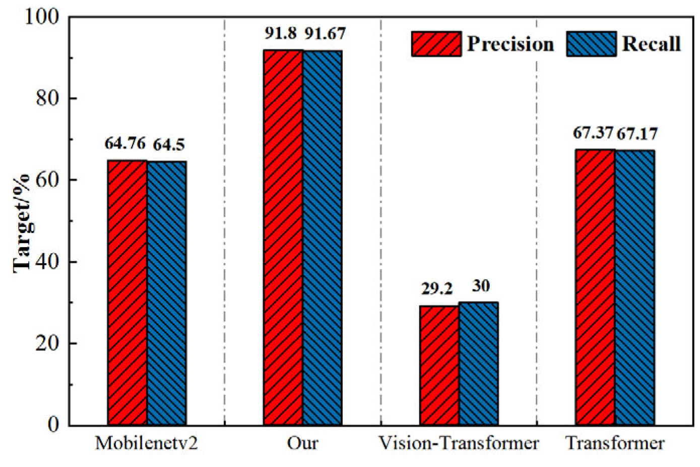
In this study, model performance is evaluated using precision and recall metrics. Precision measures the proportion of true positive instances among all instances predicted as positive by the classifier or retrieval system. Recall, on the other hand, focuses on the proportion of actual positive instances correctly identified by the classifier or system, assessing its ability to detect all true positives. A higher recall indicates that the system can effectively identify all actual positive instances. A comparison of the evaluation metrics is shown in Figure 14.

Figure 14.
Comparison of P-R Index Performance.
As shown in Figure 14, the ResNet50 algorithm proposed in this study significantly outperforms the other three algorithms. The improved performance of this model can be attributed to its deeper network architecture, which enables the learning of more complex features, along with the introduction of residual connections. These connections address the gradient vanishing problem during the training of deep networks. Each residual block contains two convolutional layers and a skip connection, which not only ensures efficient gradient propagation but also enhances the model’s training efficiency and performance. The model achieved precision and recall rates of 91.8% and 91.67%, respectively.
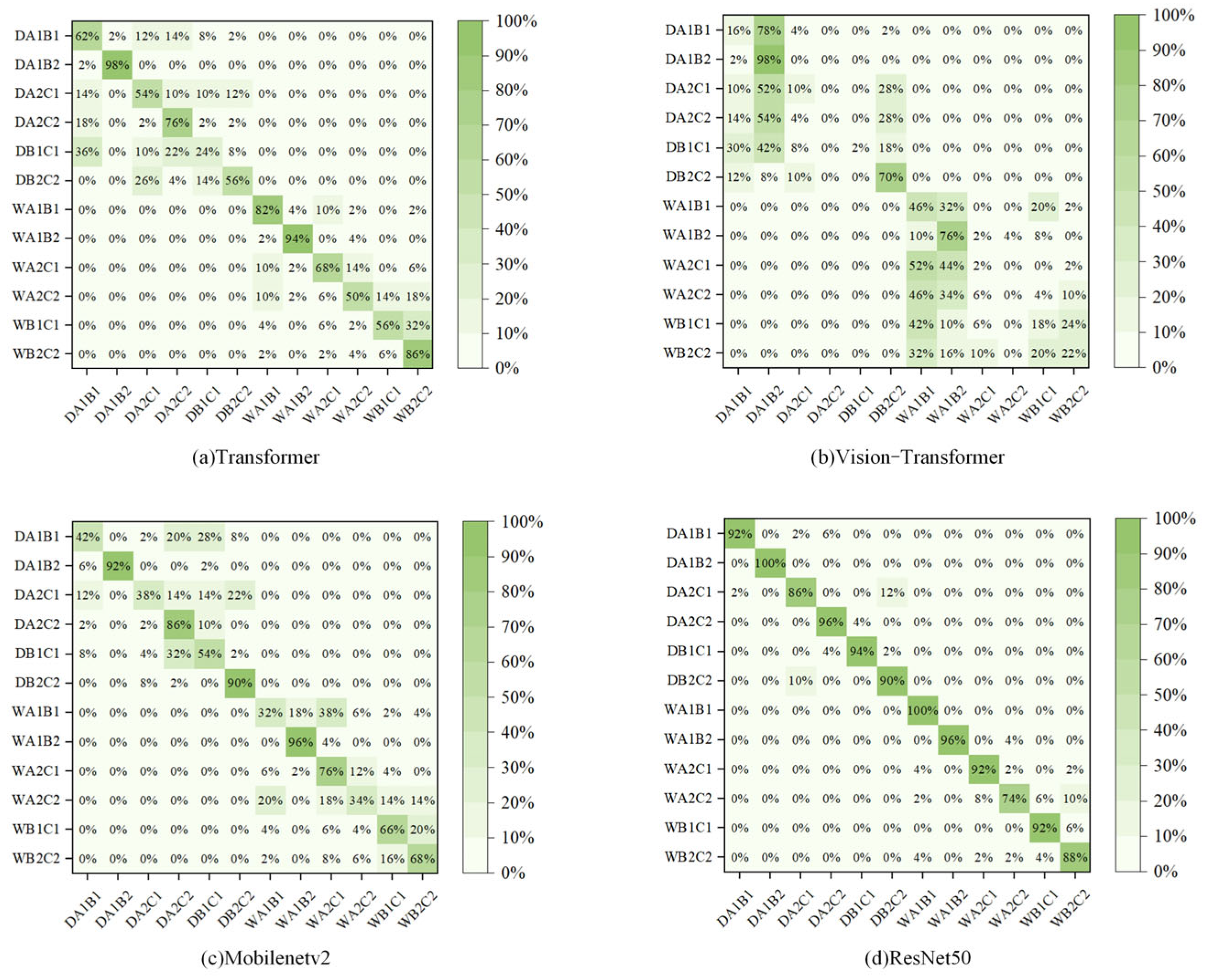
To provide a more intuitive comparison of how different algorithms perform on small-sample fault diagnosis data from the actuator mechanism, confusion matrices for all four algorithms were plotted. These matrices directly reflect the accuracy of each algorithm in recognizing signals from different fault combinations. The confusion matrix comparison for the four models is shown in Figure 15, where the horizontal axis represents the predicted labels, and the vertical axis represents the actual labels.
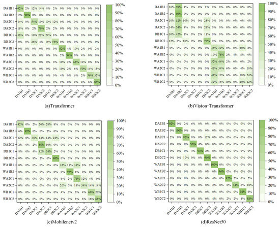
Figure 15.
Comparison of model fault diagnosis evaluation performance.
Figure 15a shows the fault diagnosis results for the Transformer model. The overall performance of this model is moderate, with accuracy rates for identifying the actuator combination fault images DA1B2, WA1B1, WA1B2, and WB2C2 being 98%, 82%, 94%, and 86%, respectively. However, the recognition rates for the remaining fault images are all below 80%.
Figure 15b shows the fault diagnosis results for the Vision Transformer model, where only the DA1B2 recognition rate reaches 98%, and the performance for other faults is poor. Among the four models, the best performance is seen in the (b) MobileNetV2 model, which also incorporates residual networks and uses depthwise separable convolutions with linear activation during dimensionality reduction. This model achieves an accuracy of over 90% for identifying DA1B2, DB2C2, and WA1B2 images, with a recognition rate of 86% for DA2C2. The (d) ResNet50 model used in this study performs the best overall. By introducing residual networks and employing standard convolutions with ReLU activation functions, and using nonlinear activation during both upsampling and downsampling, the model achieves an overall fault recognition accuracy of 91.67%. The recognition rate for the WA2C2 fault image is 74%, while all other fault images exceed 85%, with DA1B2 and WA1B1 fault images achieving perfect accuracy of 100%.
Top-1 Accuracy refers to whether the model’s predicted highest probability class matches the true class. If the model’s predicted highest probability class corresponds to the true class, the prediction is considered correct; otherwise, it is considered incorrect. Top-1 Accuracy represents the proportion of correct predictions made by the model. On the other hand, Top-5 Accuracy indicates whether the true class is within the top five predicted classes with the highest probabilities. If the true class is present in the top five predictions, the prediction is deemed correct; otherwise, it is incorrect.
As shown in Table 1, the ResNet50 model achieves the highest Top-1 Accuracy at 91.67%, followed by the Transformer model with 67.17%. The accuracies for MobileNetV2 and Vision Transformer are relatively lower, at 64.50% and 30.00%, respectively.

Table 1.
Diagnostic model comparison parameters.
In terms of parameter count (Params) and computational complexity (GFLOPs), the Swin Transformer and Vision Transformer models exhibit higher complexity, with parameter counts of 87.705 M and 86.416 M, and computational complexities of 30.340 G and 33.727 G, respectively. In contrast, the ResNet50 and MobileNetV2 models have lower complexity, with parameter counts of 25.557 M and 3.505 M, and computational complexities of 8.267 G and 0.654 G, respectively.
The ResNet50 fault diagnosis model demonstrates optimal performance in terms of accuracy, while maintaining relatively low complexity, thus achieving a balance between efficiency and performance. In contrast, although the Transformer and Vision Transformer models exhibit significantly increased complexity, they do not surpass ResNet50 in predictive accuracy, indicating that the higher resource demands do not directly translate into better performance. The MobileNetV2 model performs mediocrely in both aspects, failing to achieve top-tier accuracy, yet maintaining a lower complexity.
6. Conclusions
This paper addresses the complex mechanical failure issues faced by the CT-26 spring actuating mechanism in real-world operational environments. An innovative fault simulation strategy was designed to detect the combination of faults in the actuating mechanism, utilizing wavelet transform and deep residual networks.
- (1)
- Due to the challenges in quantitative analysis and the inadequate simulation effects in traditional core jamming fault simulations, one of the key innovations of this paper is the design and successful integration of a novel spring damping device at the core position. The ingenuity of this device lies in its ability to directly simulate the core jamming state, ensuring high fidelity and controllability during the simulation process. This significantly enhances the accuracy and practicality of fault simulations, providing an effective solution to the long-standing bottlenecks in simulation technology.
- (2)
- In this study, six types of combined faults were designed. During the fault signal preprocessing phase, the Morlet wavelet transform technique was applied to convert the current and displacement signals in the combined fault time series into images rich in time-frequency information.
- (3)
- The ResNet50 deep residual network was employed, leveraging its unique Conv-block and Identity-block modules to address the issues of gradient vanishing and explosion in the diagnosis of time-frequency data for operating mechanisms. The model’s recognition performance was enhanced through specialized downsampling and upsampling convolution strategies. An average accuracy of 91.67% was achieved in identifying twelve types of fault signals. With a parameter count of 25.557 million and a complexity of 8.267 gigaflops, computational resources and time were conserved without compromising diagnostic accuracy. This underscores the model’s high precision and efficiency in the fault diagnosis of high-voltage circuit breakers.
Author Contributions
Conceptualization, H.S.; formal analysis, H.S., Y.J., J.Z., X.L., M.Z. and M.Y.; Investigation, H.S., Y.J., J.Z., X.L., M.Z., M.Y. and X.W.; writing—original draft, X.W. and H.Y.; writing—review and editing, H.S. and H.Y. All authors have read and agreed to the published version of the manuscript.
Funding
This work was supported by the Innovation Project of China Southern Power Grid Co., Ltd. (Grant No. YNKJXM20222318 and No. YNKJXM20222388).
Data Availability Statement
Data are contained within the article.
Conflicts of Interest
Author Yang Mingkun was employed by the company Electric Power Research Institute of Yunnan Power Grid Co., Ltd. The remaining authors declare that the research was conducted in the absence of any commercial or financial relationships that could be construed as a potential conflict of interest.
References
- Popov, I.; Jenner, D.; Todeschini, G.; Igic, P. Use of the DMAIC Approach to Identify Root Cause of Circuit Breaker Failure. In Proceedings of the 2018 International Symposium on Power Electronics, Electrical Drives, Automation and Motion (SPEEDAM), Amalfi, Italy, 20–22 June 2018; pp. 996–1001. [Google Scholar]
- Yang, Q.; Ruan, J.; Zhuang, Z.; Huang, D. Chaotic analysis and feature extraction of vibration signals from power circuit breakers. IEEE Trans. Power Deliv. 2020, 35, 1124–1135. [Google Scholar] [CrossRef]
- Wang, J.; Zhang, X.; Sun, G.; Hu, W. Failure cause and handling of CD10 type electromagnetic operating mechanism. Rural. Electrif. 2005, 11, 46–48. [Google Scholar]
- Ma, Q.; Rong, M.Z.; Jia, S.L. Study of switching synchronization of high voltage breakers based on the wavelet packets extraction algorithm and short time analysis method. Proc. CSEE 2005, 25, 149–154. [Google Scholar]
- Sun, Y.H.; Wu, J.W.; Lian, S.J.; Zhang, L.M. Extraction of vibration signal feature vector of circuit breaker based on empirical mode decomposition amount of energy. Trans. China Electrotech. Soc. 2014, 29, 228–236. [Google Scholar]
- Sun, L.; Hu, X.; Ji, Y. Fault diagnosis or HV circuit breakers with characteristic entropy of wavelet packet. Autom. Electr. Power Syst. 2006, 30, 62–65. (In Chinese) [Google Scholar]
- Zhang, L.; Huang, X.; Jiang, B.; Hu, H.; Hu, X. On line monitoring technology of mechanical characteristics of circuit breaker based on contact stroke measurement. J. Xi’an Polytech. Univ. 2018, 32, 302–310. [Google Scholar]
- Razi-Kazemi, A.A.; Vakilian, M.; Niayesh, K.; Lehtonen, M. Circuit-Breaker Automated Failure Tracking Based on Coil Current Signature. IEEE Trans. Power Deliv. 2014, 29, 283–290. [Google Scholar] [CrossRef]
- Zhang, H.; Zhao, L.H.; Jing, W.; Yang, W.; Jiang, H.Y.; Zhu, L.L.; Rong, Q.; Fu, R.R. Condition assessment of the circuit breaker operating mechanism based on relief feature vector optimization and SOM network. High Volt. Appar. 2017, 53, 240–246. (In Chinese) [Google Scholar]
- Zhao, L.; Zhang, H.; Jing, W. Research onoperating mechanism performance of high voltage circuitbreaker based on thecoil current. J. Sichuan Univ. 2015, 47, 146–152. [Google Scholar]
- Chen, C.; Li, X.R. Fault diagnosis method of circuitbreaker operating mechanism based on coil currentanalysis. J. Zhejiang Univ. 2016, 50, 527–535. [Google Scholar]
- Chen, X.; Feng, D.; Lin, S. Mechanical Fault Diagnosis Method of High Voltage Circuit Breaker Operating Mechanism Based on Deep Auto-encoder Network. High Volt. Eng. 2020, 46, 3080–3088. [Google Scholar]
- Ma, H.; Xu, Y.; Wei, H.; Liu, Y. Mechanical fault diagnosis method of high voltage circuit breaker based on LVQ neural network. High Volt. Appar. 2019, 55, 30–36. (In Chinese) [Google Scholar]
- Hu, X.; Qi, M.; Ji, Y.; Yu, W. On line monitoring and fault diagnosis of high voltage circuit breakers based on radial basis function networks. Power Syst. Technol. 2001, 25, 41–44. [Google Scholar]
- Wei, W.; Shi, Y. The application of improved PSO-BP algorithm in nonlinear function approximating. Microelectron. Comput. 2017, 34, 112–115. [Google Scholar]
- Hu, Q.; Wang, R.; Zhan, Y. Fault diagnosis technology based on SVM in power electronics circuit. Proc. CSEE 2008, 28, 107–111. (In Chinese) [Google Scholar]
- Sun, Z.; Sun, Z.; Wei, J. Research on power transformer fault diagnosis hased on decision tree support vector machine algorithm. J. Electr. Eng. 2019, 14, 52–55. [Google Scholar]
- Wang, F. The Application of Decision Tree Algorithm on Fault Diagnosis System for Mechanical Equipment; Huazhong University of Science and Technology: Wuhan, China, 2013. [Google Scholar]
- Zhou, J.; Zhao, H.; Lin, S.; Si, H.; Li, B. Fault diagnosis of high-voltage circuit breaker based on optimized random forest algorithm. Electron. Meas. Technol. 2018, 41, 95–98. [Google Scholar]
- Ma, S.; Chen, M.; Wu, J.; Wang, Y.; Jia, B.; Jiang, Y. High-voltage circuit breaker faultdiagnosis using a hybrid feature transformation approach based on random forest and stacked auto-encoder. IEEE Trans. Ind. Electron. 2018, 66, 9777–9788. [Google Scholar] [CrossRef]


Disclaimer/Publisher’s Note: The statements, opinions and data contained in all publications are solely those of the individual author(s) and contributor(s) and not of MDPI and/or the editor(s). MDPI and/or the editor(s) disclaim responsibility for any injury to people or property resulting from any ideas, methods, instructions or products referred to in the content. |
© 2025 by the authors. Licensee MDPI, Basel, Switzerland. This article is an open access article distributed under the terms and conditions of the Creative Commons Attribution (CC BY) license (https://creativecommons.org/licenses/by/4.0/).