Wind Turbine Fault Diagnosis with Imbalanced SCADA Data Using Generative Adversarial Networks

Abstract

Wind turbine fault diagnostics is essential for enhancing turbine performance and lowering maintenance expenses. Supervisory control and data acquisition (SCADA) systems have been extensively recognized as a feasible technology for the realization of wind turbine fault diagnosis tasks due to their capacity to generate vast volumes of operation data. However, wind turbines generally operate normally, and fault data are rare or even impossible to collect. This makes the SCADA data distribution imbalanced, with significantly more normal data than abnormal data, resulting in a decrease in the performance of existing fault diagnosis techniques. This article presents an innovative deep learning-based fault diagnosis method to solve the SCADA data imbalance issue. First, a data generation module centered on generative adversarial networks is designed to create a balanced dataset. Specifically, the long short-term memory network that can handle time series data well is used in the generator network to learn the temporal correlations from SCADA data and thus generate samples with temporal dependencies. Meanwhile, the convolutional neural network (CNN), which has powerful feature learning and representation capabilities, is employed in the discriminator network to automatically capture data features and achieve sample authenticity discrimination. Then, another CNN is trained to perform fault classification using the augmented balanced dataset. The proposed approach is verified utilizing actual SCADA data derived from a wind farm. The comparative experiments show the presented approach is effective in diagnosing wind turbine faults.

1. Introduction

With the continuous growth of global energy demand and the increasingly serious environmental pollution problem, the utilization of wind energy has emerged as a novel, sustainable solution to the prevailing worldwide energy crisis and environmental concerns. In recent years, global installed wind capacity has continued to grow on an annual basis. Wind turbines are complicated energy conversion systems consisting of multiple components such as blades, gearboxes, hubs, and generators. To increase power generation, wind turbines are situated in high elevations and typically operate in harsh environments, making them highly susceptible to failure [1]. Unexpected wind turbine failure could cause serious economic losses and affect the stable operation of the power system [2]. Fault diagnosis of wind turbines is therefore essential to improve operational reliability and save operating and maintenance expenses.

In the last few decades, vibration-based signal processing techniques have been extensively employed to diagnose faults in key wind turbine parts, including rolling bearings [3,4], gearboxes [5], blades [6,7], etc. Additionally, because image processing techniques have significant potential for identifying damage, they have been successfully used in wind turbine fault detection, particularly blade fault detection [8,9,10]. Despite these methods being feasible and yielding accurate diagnostic outcomes, they are dependent on intricate fault mechanisms and expert knowledge. As a cost-effective approach without additional hardware investment, supervisory control and data acquisition (SCADA) systems have been extensively deployed in modern large-scale wind turbines [11]. They have the ability to real-time monitor the operating status of wind turbines, as well as provide abundant data information, including working status, monitoring parameters of subsystems and components, and so on. In SCADA systems, data collection is crucial to achieving these tasks, and it mainly relies on sensors, controllers, remote terminal units (RTUs), and programmable logic controllers (PLCs). These components work in tandem to ensure that data are efficiently and reliably collected from field devices and transmitted in real time to the monitoring center. Among them, sensors are used to measure various parameters, including temperature, pressure, etc., and the controller receives and initially processes these data. Whereas RTU or PLC serves to aggregate the data from the sensors and controllers and transmit them to the remote center. Overall, data collection in SCADA systems involves three steps. Firstly, the sensors and controllers measure various parameters and send the data to the RTU or PLC. Then, these data are received by the RTU or PLC and are initially processed and stored, and finally, are transmitted to the remote monitoring center through the communication network. Currently, there has been considerable interest in the academic community in wind turbine fault diagnosis based on SCADA data. Scholars have proposed various machine learning methods for diagnosing wind turbine faults, such as support vector machine (SVM), Gaussian process classifier (GPC), random forest (RF), and emerging deep learning technology. Zhang et al. [12] utilized the RF classifier to identify blade icing faults. Li et al. [13] built a GPC-based fault diagnosis approach and realized the recognition of different faults in wind turbines. Zhou et al. [14] employed the particle swarm optimization-based SVM to diagnose blade icing faults. Specifically, the distinct benefits of deep learning in mining hierarchical and deep feature representations have made it the mainstream technology for diagnosing wind turbine faults [15]. For instance, Pang et al. [16] created a spatio-temporal fusion neural network for diagnosing wind turbine faults by fully utilizing the spatio-temporal correlations inherent in SCADA data. Qin et al. [17] employed long short-term memory networks (LSTMs) and attention mechanisms to diagnose faults in wind turbine pitch systems. Jiang et al. [18] used convolutional neural networks (CNNs) to identify different failure categories in wind turbine gearboxes. Liu et al. [19] developed a fault detection model with deep autoencoders and ensemble techniques to identify blade icing faults. The above studies provide reliable diagnostic classification performance. Nevertheless, they have the same number of samples for different health conditions during training, which is limited in practical applications.

Wind turbines operate normally most of the time and are not permitted to operate for extended periods of time in the event of failures. In addition, the frequency of failures significantly varies among various subsystems and components [20]. This leads to the phenomenon of data imbalance, characterized by an abundance of normal data relative to abnormal data. In such cases, the fault diagnosis model is generally inclined to favor the majority class, that is, normal data, which causes the performance of fault diagnostics to decline. Consequently, to deal with the data imbalance issue, various data generation methods, including undersampling [21], oversampling [22], and synthetic minority oversampling technology (SMOTE) [23,24], have been proposed to obtain balanced datasets. The fundamental idea of the former two methods is to balance the data distribution through undersampling the majority classes and oversampling the minority classes. On the other hand, SMOTE, as a specific oversampling method, aims to interpolate between a given minority class sample and adjacent samples to produce new unduplicated samples. However, these sampling methods have certain drawbacks, such as losing samples that contain valuable information or, alternatively, overfitting the classification model to the training data and reducing the generalization ability of the model. In particular, compared to the above approaches, generative adversarial networks (GANs) are able to learn more abundant data distributions and create additional, more realistic data in an unsupervised learning manner [25]. It adopts the adversarial learning strategy in the training process and has been successfully used to deal with data imbalance problems in various fields, such as image classification [26], pearl classification [27], and face recognition [28]. In addition, GANs have shown significant potential in the application of class imbalance in wind turbine fault diagnosis. For example, Liang et al. [29] utilized data augmentation GANs to learn the distributions of extracted two-dimensional image data and generate extended samples, and then a capsule neural network was used to diagnose wind turbine gearbox faults, thus providing higher diagnostic performance. Guo et al. [25] first performed the preprocessing of the raw data using wavelet packet decomposition, and then Wasserstein distance with gradient punishment was employed to enhance the adversarial learning capacity of conditional GANs, realizing the accurate identification of gearbox failures. Su et al. [30] established a Wasserstein GAN fault diagnosis model based on a kurtosis perceptron, a genetic algorithm, and a logistic regression auxiliary classifier, which was effectively used to identify gearbox faults with imbalanced datasets. Chen et al. [31] built a Bayesian-GAN-LSTM-based diagnosis approach, which achieved the generation of bearing data and obtained accurate and robust diagnostic results. However, the abovementioned GAN-based wind turbine fault diagnosis methods principally focus on vibration data and heavily rely on feature extraction, and there are limitations of GANs for data generation and fault diagnosis in SCADA data.

As mentioned above, wind turbines are complex electromechanical systems with variable working environments, resulting in the SCADA monitoring data with complex and diverse characteristics. In addition, SCADA monitoring variables have typical temporal characteristics. Therefore, it is challenging to construct a suitable GAN model to generate data and identify wind turbine faults for imbalanced, complex, multivariate time series data. To tackle this problem, a fault diagnosis method based on deep learning for wind turbines with imbalanced data is proposed in this paper, which includes two stages of data generation and fault classification. Firstly, a generative adversarial network combining LSTM and a CNN (LCGAN) is established for the purpose of learning the distributions of real SCADA data samples. Specifically, considering the temporal correlation inherent in the SCADA data, LSTM is used in the generator network to generate samples with temporal dependencies. Meanwhile, the CNN has excellent feature learning and representation capabilities, which can automatically discover and extract discriminative features from data and is employed in the discriminator network for sample authenticity discrimination. This process enables the generation of additional realistic fake samples, thus balancing the training dataset. Subsequently, an additional CNN model is trained for fault classification through the use of the augmented balanced dataset. The contributions of this paper can be summarized as follows:

• A novel LCGAN data generation model is proposed to learn the distributions of the real SCADA data samples and deal with the class imbalance problem. Afterwards, an additional CNN model is built to perform the fault classification task using the augmented dataset. The proposed fault diagnosis approach integrating LCGAN data generation and CNN fault classification can enhance the fault diagnosis performance.
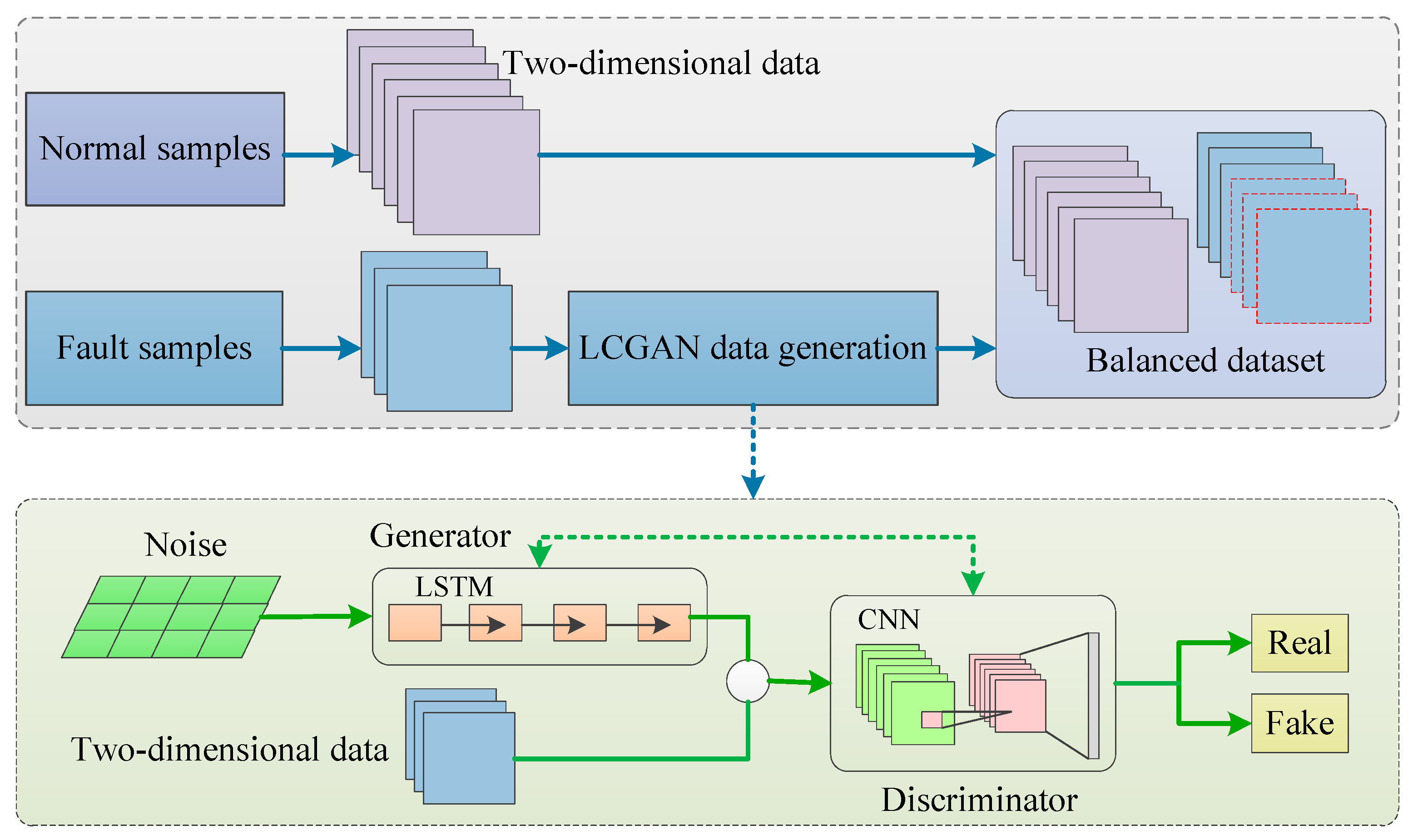
• In the proposed LCGAN model, generator and discriminator networks are designed separately. Specifically, LSTM is used in the generator network to learn the temporal correlations from SCADA data, thereby creating samples with temporal dependencies. Moreover, the CNN is employed in the discriminator network to extract complex feature representations, enabling better judgment of the authenticity of the samples. And data can be generated through continuous adversarial learning between the two networks.
• The efficacy of the proposed fault diagnosis approach is confirmed using SCADA data from actual wind turbines, and comparative experiments are performed.

The remaining sections are organized as follows. Section 2 reviews the theoretical background of the GAN model. Section 3 gives a comprehensive overview of the proposed method for fault diagnosis. Section 4 validates the proposed method using real data. Section 5 draws the conclusion of this article.

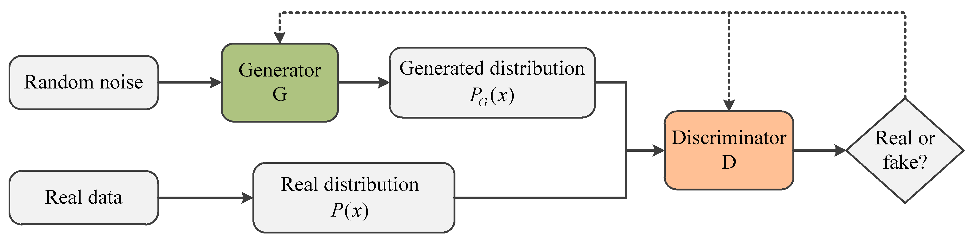
2. Theoretical Background of Generative Adversarial Networks

As an emerging generative model, generative adversarial networks were introduced by Goodfellow et al. [32] in 2014. In contrast to traditional supervised models, this model is an unsupervised deep learning model that comprises two mutually independent modules, generator G and discriminator D. These two networks compete with each other and improve. By adopting adversarial training strategies, samples that are closer to real data can be generated based on a small amount of available data to handle the data imbalance problem. In addition, both the generator and the discriminator are composed of neural networks, and the appropriate network structure can be adjusted according to the characteristics of the data, which largely improves the degree of freedom in model design. As mentioned in Section 1, GANs have been effectively used for data generation in various tasks, including image classification, face recognition, and wind turbine fault diagnosis, in recent years. However, it is worth noting that the model itself has certain limitations, such as difficulty in training and relatively large amounts of training data.

Figure 1 presents the basic GAN structure. Among them, the generator G network produces a new probability distribution $P_G(x)$ according to the probability distribution $P(x)$ of the actual data, and the discriminator D network seeks to discriminate $P_G(x)$ and $P(x)$. During the training of the GAN, the noise vector $z$ is fed into the generator network to produce $P_G(x)$, which is then input into the discriminator network along with $P(x)$ to discriminate, and the loss values are computed. Based on this result, these two networks are retrained. It should be noted that the two networks are simultaneously trained. On the one hand, the training of the generator attempts to create data that can trick the discriminator. On the other hand, the discriminator is trained to differentiate between actual and produced data. Through continuous adversarial learning between the G and D, the discriminator is optimized to correctly differentiate between actual and produced data, and conversely, the generator is updated to produce realistic data that cannot be recognized by the discriminator [33]. Thus, the GAN can achieve the goal of data augmentation. The objective function of the GAN model is defined as

$$\underset{G}{\min }\underset{D}{\max }V(D,G)=E_{x\sim P_{data}}[\log (D(x)]+E_{z\sim P_z}[\log (1-D(G(z)))],$$

(1)

where $x$ refers to the real data and $G(z)$ is the generated data. $E_{x\sim P_{data}}$ and $E_{z\sim P_z}$ denote the distribution of the real data and fake data, respectively.

3. Proposed Wind Turbine Fault Diagnosis Method

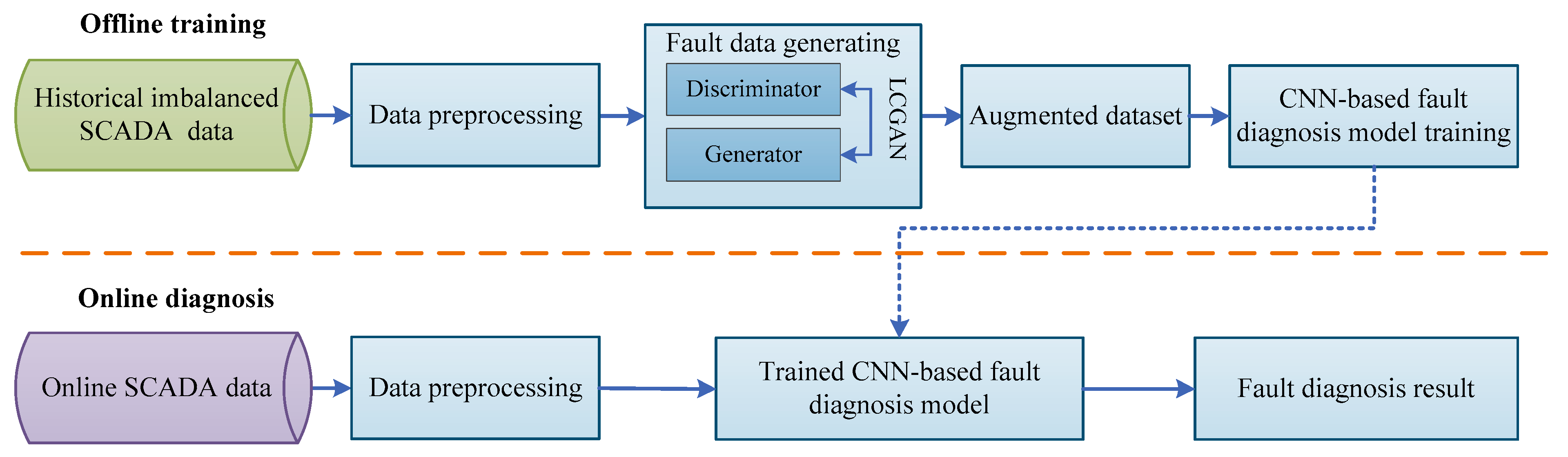
3.1. Overview of the Proposed Method

The overall schematic of the proposed wind turbine fault diagnosis with imbalanced SCADA data is shown in Figure 2. Generally, in order to realize effective fault identification, it is essential to include more fault data to cover all potential wind turbine conditions. However, this is not easy to carry out in practice because of the scarcity or even unavailability of the fault data. Hence, the fundamental principle underlying the proposed methodology is the augmentation of fault data only and then forming a balanced dataset with the original normal data to execute the fault diagnosis task. To this end, this paper introduces an LCGAN data generation method, in which an LSTM network with good learning time dependence and a CNN with strong feature characterization capability are employed in generator and discriminator networks, respectively. The proposed LCGAN data generation model has the capacity to mine the underlying distributions of the SCADA multivariate time series data using available fault data. Consequently, additional realistic fake fault data are produced to augment the training dataset. In addition, regarding the fault classification step, the CNN model is also used to enhance the classification performance. It is noteworthy that the proposed fault diagnosis approach is general and suitable for generating data on different fault types of wind turbines and conducting fault classification. To be specific, the proposed wind turbine fault diagnosis method comprises offline training and online diagnosis, and the detailed procedure is outlined below.

• Offline training phase: Historical imbalanced SCADA data with normal and fault conditions are first collected. For different health conditions, necessary data preprocessing, including data normalization as well as two-dimensional fragment segmentation, is then carried out. Further, the LCGAN model is employed to produce fault data. These produced data are then merged into the original imbalanced dataset for data augmentation. At last, based on the expanded balanced dataset, the CNN-based fault diagnosis model is trained for wind turbine fault classification and identification.
• Online diagnosis phase: Online SCADA data are acquired and then preprocessed in the same manner as in the offline phase. Afterwards, the data are entered into the CNN-based fault classification model that has been adequately trained to automatically determine the health condition it belongs to and give the fault classification results.

3.2. LCGAN-Based Data Generation

In this study, the distribution of the fault data is explored using the LCGAN-based approach, and additional realistic fake data are produced from the noise. At this point, the original imbalanced dataset is balanced by the addition of produced fault samples, which are subsequently employed to implement the fault classification task to enhance the diagnostic performance. Specifically, the input to the LCGAN model is two-dimensional multivariate time series data that have been preprocessed. In addition, two different health conditions, namely normal and single fault, are investigated in this study for fault diagnosis, belonging to a typical binary classification problem. Figure 3 shows the framework of the data generation stage.

As shown in Figure 3, for the purpose of balancing the normal and fault data, a generative adversarial network is employed in the LCGAN data generation module, including a generator and a discriminator. In particular, with regard to the generator model, considering that the SCADA data have the temporal characteristic, LSTM, which is capable of handling time series data well, is adopted for better learning of temporal information and improving the quality of the produced data. It is worth mentioning that during the training of the LCGAN, the pre-training of the generator is executed first. Random noise is fed into the LSTM network, and the corresponding data are generated. Subsequently, the mean square error between the generated data and the real data is calculated to update the network parameters. By performing several iterations, the pre-training process is completed.

LSTM is a specialized form of a recurrent neural network (RNN) that was presented by Hochreiter and Schmidhuber [34] to address the gradient vanishing problem that exists in traditional the RNN. Unlike the traditional RNN, LSTM includes not only the hidden state vector $h_t$ but also a memory cell $c_t$ that is mainly controlled by three gates: input gate $i_t$, forget gate $f_t$, and output gate $o_t$. Figure 4 displays the structure of the LSTM network. The updating equations are described as follows:

$$i_t=\mathrm{sigmoid}(U_i{h}_{t-1}+W_i{x}_t+b_i),$$

(2)

$$f_t=\mathrm{sigmoid}(U_f{h}_{t-1}+W_f{x}_t+b_f),$$

(3)

$$o_t=\mathrm{sigmoid}(U_o{h}_{t-1}+W_o{x}_t+b_o),$$

(4)

$${\tilde{c}}_t=\tan \mathrm{h}(U_c{h}_{t-1}+W_c{x}_t+b_c),$$

(5)

$$c_t=f_t\odot c_{t-1}+i_t\odot {\tilde{c}}_t,$$

(6)

$$h_t=o_t\odot \tanh (c_t),$$

(7)

where all $U\in {ℝ}^{d\times d}$, $W\in {ℝ}^{d\times k}$, and $b\in {ℝ}^d$ represent learnable parameters, and the operator $\odot$ refers to the element-wise multiplication. At time step $t$, the forget gate $f_t$, input gate $i_t$, and output gate $o_t$ are formed by a function of the new input $x_t$ and previous hidden state $h_{t-1}$, respectively. Among them, the forget gate $f_t$ determines how much of the last memory cell $c_{t-1}$ is retained in the current memory cell $c_t$. When the value of the forget gate approaches 1, information from the last memory cell $c_{t-1}$ will be retained, and vice versa. The input gate $i_t$ determines how much of the current input $x_t$ is kept in the memory cell $c_t$, while the output gate $o_t$ is used to control how much of the memory cell $c_t$ is output to the current hidden state $h_t$.

In order to enhance the capacity of the discriminator network to capture data features and effectively differentiate between true and false data, a CNN, which has powerful automatic feature learning and classification capability, is adopted. The generated data and real data are input into this network, where corresponding convolution and pooling operations are performed. These operations can extract important characteristics, and the data source is accurately determined through continuous optimization.

A CNN is a kind of feed-forward neural network developed under the inspiration of biological neurology, aiming at imitating the behavior of the mammalian visual cortex [18]. The network was originally proposed by Lecun et al. [35] for handwritten digit recognition. Currently, the CNN has been successfully used in different application fields with its powerful feature-learning and representation capabilities. Compared with traditional fully connected neural networks, the CNN is characterized by weight-sharing and sparse connectivity. With these two features, the amount of training parameters can be drastically reduced, and the risk of overfitting can be mitigated [36]. The construction of the CNN is shown in Figure 5 and consists of the convolutional layer, pooling layer, and fully connected layer. The convolutional layer is designed to capture local features by performing the convolution operation on the input data with multiple different convolution kernels. The convolution operation is described as

$$x_j^l=f({\displaystyle \sum _i{x}_i^{l-1}}\ast k_{ij}^l+b_j^l),$$

(8)

where $x_j^l$ refers to the $j\mathrm{th}$ feature map at the $l\mathrm{th}$ layer, $x_i^{l-1}$ is the $i\mathrm{th}$ input feature map at the $(l-1)th$ layer, $k_{ij}^l$ is the convolution kernel connecting the $i\mathrm{th}$ input feature map with the $j\mathrm{th}$ feature map, $b_j^l$ represents the bias term, $\ast$ denotes the convolution operation, and $f(\cdot )$ stands for the nonlinear activation function. In this paper, rectified linear unit (ReLU) is selected as the activation function, which is expressed as $f(x)=\max (0,x)$.

The pooling layer generally appears after the convolutional layer, where redundant data features are eliminated through pooling operations so that the most critical information is retained and computational efficiency is improved. The most frequently employed pooling techniques are maximum pooling and average pooling. In this paper, global average pooling is added to the discriminator network to minimize overfitting. Subsequently, the fully connected (FC) layer integrates the obtained local information, with each neuron in this layer being fully connected to all neurons in its adjacent layers.

3.3. Fault Classification

In the fault classification stage, the backbone is the convolutional neural network aimed at automatically learning valuable fault information from large amounts of complex SCADA data and consequently improving fault classification performance. The balanced dataset obtained in the LCGAN data generation stage is directly fed into the CNN for training to perform fault classification between normal and fault behaviors. Note that the classification problem for the wind turbine fault diagnosis studied in this article belongs to a typical supervised learning scheme and is a binary classification problem indicating whether the wind turbine is operating normally. During the model training, the cross-entropy between the actual and predicted class labels is chosen as the loss function, which is expressed as

$$H(p,q)=-{\displaystyle \sum _{i}p(i)\log q(i)},$$

(9)

where $p(i)$ represents the true distribution and $q(i)$ refers to the estimated distribution. Finally, following sufficient training, the performance of the presented classification approach is verified using the test data.

4. Experimental Verification

In this section, the presented approach is utilized to identify actual wind turbine blade icing faults, which are a common fault in turbines. It is well known that in order to make the best use of wind energy, wind turbines tend to be built on high ground and subjected to low temperature and high humidity climatic conditions, which makes the blades easily frozen in cold climates, particularly during winter months. Ice accretion on blades has an impact on the ability of wind turbines to generate electricity, and in severe cases, it can lead to a loss of up to 30% in annual power generation while also bringing safety risks to the surrounding areas of the wind farm [37]. Therefore, the blade icing fault scenario is considered and investigated, and the experimental results and comparative experiments are presented and analyzed.

4.1. Data Description

The SCADA data available for this study derive from two wind turbines situated within an actual wind farm in Inner Mongolia, China [38]. The monitoring data recorded by these two wind turbines represent a running time of 305.77 h and 695.59 h, respectively. The data are acquired at 7 s intervals. Hundreds of sensor measurements are captured by the wind turbine SCADA system, which are mainly measured through anemometers, temperature sensors, speed sensors, acceleration sensors, angle sensors, etc. As shown in

Table 1. Specified sensor variables.

No.	Variable Description	No.	Variable Description
1	Wind speed	14	Temperature of pitch motor 1
2	Generator speed	15	Temperature of pitch motor 2
3	Active power	16	Temperature of pitch motor 3
4	Wind direction	17	Horizontal acceleration
5	Average wind direction angle within 25 s	18	Vertical acceleration
6	Yaw position	19	Environmental temperature
7	Yaw speed	20	Internal temperature of nacelle
8	Angle of pitch 1	21	Switching temperature of pitch 1
9	Angle of pitch 2	22	Switching temperature of pitch 2
10	Angle of pitch 3	23	Switching temperature of pitch 3
11	Speed of pitch 1	24	DC power of pitch 1 switch charger
12	Speed of pitch 2	25	DC power of pitch 2 switch charger
13	Speed of pitch 3	26	DC power of pitch 3 switch charger

, 26 variables related to blade icing are specified, and the data are labeled as icing or normal. In general, these 26 variables involve wind parameters (e.g., wind speed, wind direction), temperature parameters (e.g., environment temperature, pitch motor temperature, nacelle temperature), energy-related parameters (e.g., generator speed, yaw speed, pitch angle), and vibration parameters (e.g., horizontal acceleration, vertical acceleration).

The raw data used in this paper are multiple multivariate time series segments with a fixed length of 512, each of which represents the status of the turbine for nearly 1 h. In addition, these data have been normalized to a specified range to minimize the impact of different units. To improve computational efficiency, herein, these data are further divided into segments of length 128, which indicates that each segment represents a sequence of 15 min. That is, the original segment is equally separated into four parts along the time axis, and the duplicate segments existing in the abnormal dataset are deleted after processing. At this point, a total of 3360 normal condition samples and 1472 blade icing samples are obtained. These samples are then further partitioned into training and testing sets, which are used to train and assess the performance of the proposed method, respectively. For the normal condition, 3000 samples are selected at random to serve as the training data, and the rest of the 360 samples are used as the testing data. In the same manner, random 360 samples of the fault condition are chosen as testing data, with the remainder serving as the training data. The detailed description of the training and testing data is summarized in

Table 2. Detailed descriptions of the training and testing data.

Condition	Size of Training Data	Size of Testing Data
Normal	3000	360
Fault	1112	360

. Notably, the training data are imbalanced, while the testing data are balanced.

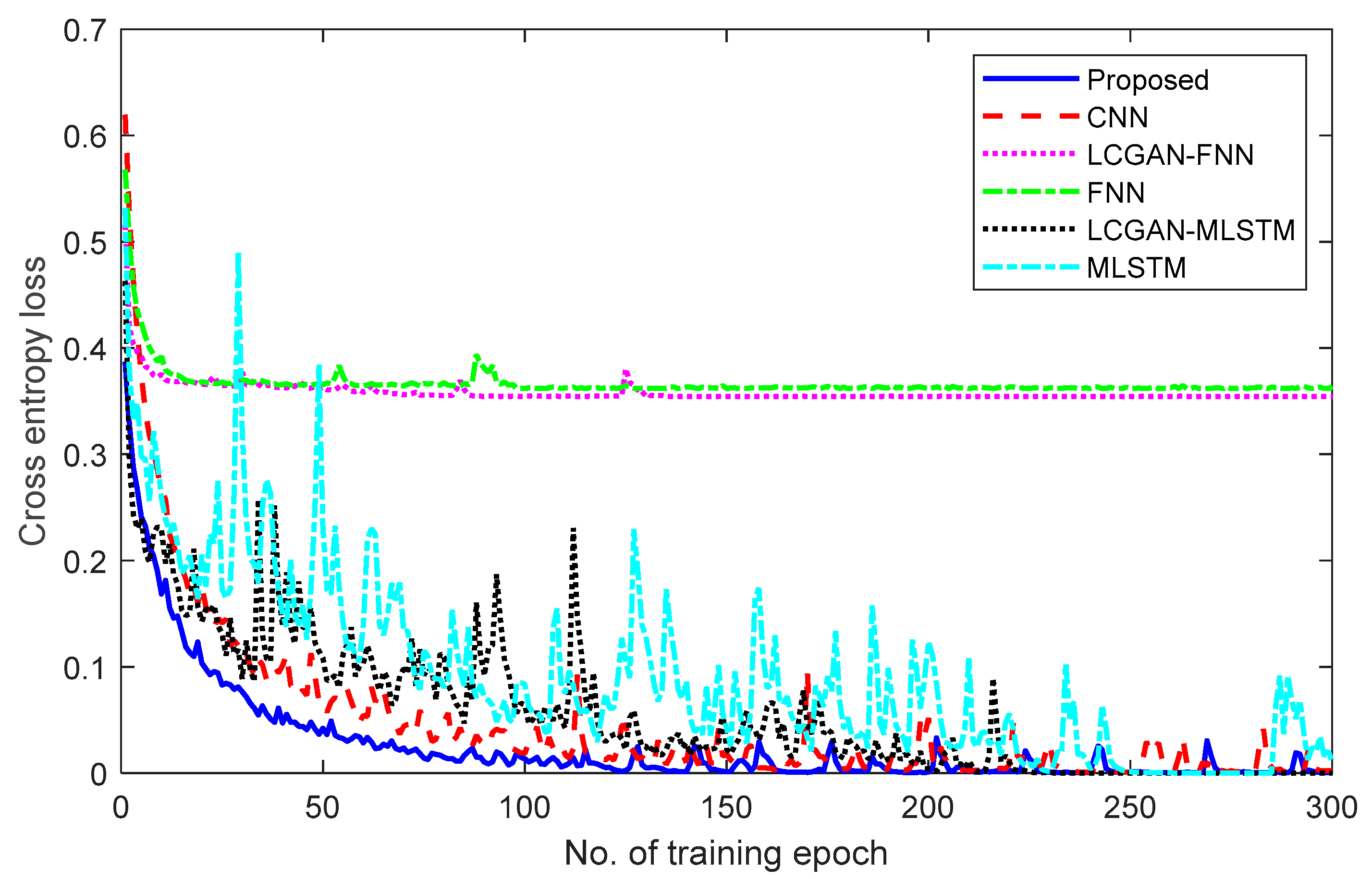
4.2. Experimental Results and Analysis

In this section, four widely used evaluation metrics, accuracy, precision, recall, and F1 score, are adopted to assess and compare the performance of the proposed wind turbine fault diagnosis method. These metrics are described as follows:

$$\mathrm{Accuracy}={\displaystyle \frac{\mathrm{TP}+\mathrm{TN}}{\mathrm{TP}+\mathrm{FN}+\mathrm{FP}+\mathrm{TN}}},$$

(10)

$$\mathrm{Precision}={\displaystyle \frac{\mathrm{TP}}{\mathrm{TP}+\mathrm{FP}}},$$

(11)

$$\mathrm{Recall}={\displaystyle \frac{\mathrm{TP}}{\mathrm{TP}+\mathrm{FN}}},$$

(12)

$$\mathrm{F}1\mathrm{-score}={\displaystyle \frac{2\times \mathrm{Precision}\times \mathrm{Recall}}{\mathrm{Precision}+\mathrm{Recall}}},$$

(13)

where $\mathrm{TP}$ and $\mathrm{TN}$ indicate the number of correctly classified positive and negative samples, and $\mathrm{FP}$ and $\mathrm{FN}$ refer to the number of misclassified positive and negative samples, respectively. Here, the normal condition is viewed as the negative class and the fault condition as the positive class.

As described in Section 3.2, to balance normal and fault datasets, the generator composed of the LSTM network and the discriminator composed of the CNN are designed in the proposed LCGAN data generation module. Specifically, two LSTM layers and a fully connected layer are employed in the generator branch. While the discriminator branch contains three successive convolutional layers, a pooling layer, and a fully connected layer [38], the sigmoid activation function is adopted to map the output values to [0, 1]. To reduce the number of parameters and prevent overfitting, a batch normalization (BN) layer follows each convolutional layer. In the process of generator pre-training, the mean square error between the generated data and the real data is used as the loss function. Moreover, the cross-entropy error is applied to update the network parameters during the training of the generator and discriminator. For all model training, the Adam optimizer is employed for the purpose of network optimization. The learning rates to pre-train the generator and train the LCGAN are 0.0005 and 0.0002, and the number of epochs is 1000 and 2000, respectively. The batch size is set to 32.

Table 3. The configuration of LSTM and CNN parameters.

Describe	Layer	Hidden Size/Filter	Kernel Size	Stride	Padding
Generator LSTM	LSTM	128
	LSTM	128
	FC	128
Discriminator CNN	Conv2D	128	(8,8)	1	same
	BN
	Conv2D	256	(5,5)	1	same
	BN
	Conv2D	128	(3,3)	1	same
	BN
	Global_avg_pool2D
	FC	1

gives details of the network structure parameters.

In addition, during the supervised fault classification phase, the CNN is used to evaluate classification performance, as mentioned in Section 3.3. In this model, two convolutional layers are first adopted, followed by a pooling layer and a fully connected layer. The BN layer is also applied after the convolutional layer. The Adam optimizer is used to train the CNN model at a learning rate of 0.0005. The number of training epochs is set to 300, and the batch size is 64.

Table 4. The configuration of fault classification network parameters.

Layer	Hidden Size/Filter	Kernel Size	Stride	Padding
Conv2D	64	(8,8)	1	same
BN
Conv2D	128	(5,5)	1	same
BN
Global_avg_pool2D
FC	2

provides detailed network structure parameters.

After the LCGAN-training process is completed, blade icing samples can be generated using the well-trained generator and discriminator parameters. A total of 2000 samples are generated in this study, and 1888 samples are randomly selected to form the fault dataset with real blade icing samples. At this point, the dataset used to train the classification model is balanced, which consists of 3000 samples of normal behavior and samples of fault behavior, i.e., a total of 6000 samples.

In this study, the LCGAN-based data generation is one of the main factors in achieving effective fault diagnosis. In order to reflect the impact of data augmentation, the classification results of the balanced training dataset augmented with the LCGAN are compared with the imbalanced training dataset without considering data augmentation. That is, the model without the data augmentation technique only includes the CNN fault classification module, while the LCGAN data generation module is discarded. The structural parameters are the same as in Table 4. Additionally, comparisons are carried out using the fully connected neural network (FNN) and multivariate LSTM (MLSTM), which are trained on augmented and nonaugmented datasets. For the FNN model, there are four fully connected layers, and the number of neurons is 512, 256, 128, and 2, respectively. The ReLU activation function is utilized, and the softmax function is employed for classification. In terms of the MLSTM, it consists of two LSTM layers, each with 64 hidden units, and one fully connected layer with two neurons. For the FNN and MLSTM training, the cross-entropy function is chosen as the loss function. The models are optimized by the Adam optimizer with a learning rate of 0.0001 and 0.001, respectively. The number of training epochs is 300, and the size of the batch is 64. The training loss curves for the different models are shown in Figure 6. The average testing results over five trials are shown in

Table 5. Diagnosis performance comparison of different methods (%).

Method	Accuracy	Precision	Recall	F1-Score
FNN	81.47	93.02	68.06	78.60
LCGAN-FNN	82.11	94.13	68.50	79.29
MLSTM	97.55	97.72	97.39	97.55
LCGAN-MLSTM	98.25	98.23	98.28	98.25
CNN	98.69	97.92	99.50	98.70
Proposed	99.64	99.28	100	99.64

and Figure 7.

As shown in Figure 6, with regard to the cross-entropy loss, the proposed LCGAN-CNN achieves smaller loss values compared to the CNN method. As the number of training epochs rises, the loss value gradually approaches 0, with relatively small fluctuations. Compared with the MLSTM, the loss value of the LCGAN-MLSTM is relatively small. Both can converge to around 0, but the fluctuation amplitude is significantly large. Although LCGAN-FNN and FNN have faster convergence speeds, the loss value converges to around 0.36 instead of 0, and the loss value of FNN is slightly higher than that of LCGAN-FNN. This indicates that the presented approach produces better learning ability and extracts more effective fault features than other methods.

As indicated in Table 5 and Figure 7, the LCGAN-FNN and LCGAN-MLSTM methods using the data augmentation technique achieve higher metric values in comparison with the FNN and MLSTM methods trained with the imbalanced dataset. The LCGAN-FNN and LCGAN-MLSTM models achieve better diagnostic performance than the FNN and MLSTM models. Moreover, the CNN model is superior to the FNN and MLSTM models. This is mainly due to the fact that the CNN model has powerful automatic feature representation and classification capabilities, thus yielding relatively good performance. Although the CNN model produces high values on all the evaluation metrics, since it uses the imbalanced dataset during training, the performance is inferior to the proposed method that incorporates the dataset balancing. In other words, the proposed data generation model further enhances the diagnostic performance. In general, compared with other methods, the presented method integrating the LCGAN data generation and the CNN fault classification obtains the best diagnostic performance, demonstrating its superiority in diagnosing wind turbine faults.

In the present study, to show the computational efficiency of different diagnostic models, the training and testing time is calculated, and

Table 6. Cost time of different models.

Method	Training Time (s)	Testing Time (s)
FNN	40.28	0.01
LCGAN-FNN	124.47	0.02
MLSTM	43.49	0.01
LCGAN-MLSTM	65.10	0.01
CNN	836.94	0.16
Proposed	1272.32	0.19

provides the calculation results. Note that all the models are implemented on the Inter Core (TM) i7 CPU with 2.3 GHz and an NVIDIA GeForce RTX 3060 GPU using the Python-3.8.10 environment on a 64-bit Windows operating system. As far as the training time is concerned, the CNN-based models take more time than the FNN-based and MLSTM-based models. In particular, the proposed method consumes the most time among all the models. This is because more training samples are considered, and a more complex model needs to be trained. However, as described in Section 3.1, every model is first learned offline and subsequently used to diagnose faults in real time. In this respect, the loss of computing time is acceptable. During the testing phase, there is no significant difference in the time taken by the six models, and the proposed method only takes 0.19 s, making it suitable for online fault diagnosis.

From an alternative standpoint, the confusion matrix of the testing diagnosis results from five experiments is presented in Figure 8, with the objective of investigating the classification performance of different methods. It indicates the samples that are correctly and incorrectly categorized for different health conditions. In this study, the normal and fault conditions are denoted by 0 and 1, respectively. As observed in Figure 8, the FNN model misclassifies the greatest number of samples for each condition. Specifically, a significant proportion of fault samples are misclassified as normal samples. After expanding the samples of the training dataset, the LCGAN-FNN model produces fewer misclassified samples, but it is still much higher than those generated by the MLSTM, LCGAN-MLSTM, CNN, and LCGAN-CNN models. This is because the traditional FNN is difficult to effectively extract and identify fault features, resulting in poor diagnostic performance. Compared with LCGAN-MLSTM, MLSTM, LCGAN-CNN, and CNN, it can be found that fewer samples are misclassified when the LCGAN data generation module is used. Especially for the proposed model, all the fault samples are accurately predicted without being misclassified. This further illustrates the efficacy of the fault diagnosis methodology presented in this paper.

5. Conclusions

A novel approach to fault diagnosis based on deep learning is put forward with the aim of addressing the issue of degraded diagnostic performance due to the imbalanced SCADA data. The main method behind this is the generative adversarial network, which consists of two phases: data generation (LCGAN) and fault classification. On the one hand, the data generation module is used for data augmentation of the fault samples, where the generator is composed of the LSTM network that can handle the time dependency well, while the discriminator adopts the CNN with powerful feature extraction capabilities. Through the continuous adversarial learning between the generator and the discriminator, new fault samples are produced to balance the training dataset. On the other hand, an additional CNN is employed to handle the fault classification problem. The balanced training dataset is then utilized to train the CNN to classify between normal and fault conditions. A case of blade icing acceleration faults is applied to evaluate the performance of the presented methodology by using actual SCADA data. Compared with the CNN model that ignores the dataset balancing and the FNN-based and MLSTM-based networks, the proposed model combining the LCGAN data generation and the CNN classification produces fewer misclassified samples and therefore achieves better diagnostic performance.

Despite the improvements in the diagnostic performance, there are certain limitations in the current work. Due to the limited SCADA data, this study is constrained to using only blade icing faults to validate the proposed methodology and does not involve other fault types in wind turbines. In addition, although there is an imbalance between normal and fault samples in the training dataset, the difference in number is not particularly significant. In future work, more SCADA operational data with multiple types of faults will be obtained to further determine the effectiveness of the proposed method in diagnosing other faults in wind turbines. To better reflect the suitability of the presented approach in highly imbalanced SCADA data, fewer fault data need to be considered. Meanwhile, it makes sense to develop more advanced generative adversarial network models to further explore the complicated correlations hidden in the SCADA multivariate time series data, thereby providing more rational diagnostic decisions for wind turbine maintenance. Furthermore, the proposed methodology can be extended to diagnose faults in other systems than wind turbines.

References

1. Rahimilarki, R.; Gao, Z.; Jin, N.; Zhang, A. Convolutional neural network fault classification based on time-series analysis for benchmark wind turbine machine. Renew. Energy 2022, 185, 916–931. [Google Scholar] [CrossRef]
2. Takoutsing, P.; Wamkeue, R.; Ouhrouche, M.; Slaoui-Hasnaoui, F.; Tameghe, T.A.; Ekemb, G. Wind turbine condition monitoring: State-of-the-art review, new trends, and future challenges. Energies 2014, 7, 2595–2630. [Google Scholar] [CrossRef]
3. Yi, C.; Yu, Z.; Lv, Y.; Xiao, H. Reassigned second-order synchrosqueezing transform and its application to wind turbine fault diagnosis. Renew. Energy 2020, 161, 736–749. [Google Scholar] [CrossRef]
4. Huang, J.; Cui, L.; Zhang, J. Novel morphological scale difference filter with application in localization diagnosis of outer raceway defect in rolling bearings. Mech. Mach. Theory 2023, 184, 105288. [Google Scholar] [CrossRef]
5. Rusmir, B.; Ninoslav, Z.; Alexandros, S.G.; Nenad, M. Feature extraction using discrete wavelet transform for gear fault diagnosis of wind turbine gearbox. Shock Vib. 2015, 2016, 6748469. [Google Scholar]
6. Sun, S.; Wang, T.; Yang, H.; Chu, F. Damage identification of wind turbine blades using an adaptive method for compressive beamforming based on the generalized minimax-concave penalty function. Renew. Energy 2022, 181, 59–70. [Google Scholar] [CrossRef]
7. Joshuva, A.; Sugumaran, V. Fault diagnosis of wind turbine blade using vibration signals through j48 decision tree algorithm and random tree classifier. Int. J. Contr. Theory Appl. 2016, 9, 249–258. [Google Scholar]
8. Rizk, P.; Rizk, F.; Karganroudi, S.S.; Ilinca, A.; Younes, R.; Khoder, J. Advanced wind turbine blade inspection with hyperspectral imaging and 3D convolutional neural networks for damage detection. Energy AI 2024, 16, 100366. [Google Scholar] [CrossRef]
9. Rizk, P.; Younes, R.; Ilinca, A.; Khoder, J. Wind turbine ice detection using hyperspectral imaging. Remote Sens. Appl. 2022, 26, 100711. [Google Scholar] [CrossRef]
10. Alvela Nieto, M.T.; Gelbhardt, H.; Ohlendorf, J.H.; Thoben, K.D. Detecting ice on wind turbine rotor blades: Towards deep transfer learning for image data. In Proceedings of the 6th International Conference on System-Integrated Intelligence (SysInt 2022), Genova, Italy, 7–9 September 2022; pp. 574–582. [Google Scholar]
11. Dao, P.B. Condition monitoring and fault diagnosis of wind turbines based on structural break detection in SCADA data. Renew. Energy 2022, 185, 641–654. [Google Scholar] [CrossRef]
12. Zhang, L.; Liu, K.; Wang, Y.; Omariba, Z.B. Ice detection model of wind turbine blades based on random forest classifier. Energies 2018, 11, 2548. [Google Scholar] [CrossRef]
13. Li, Y.; Liu, S.; Shu, L. Wind turbine fault diagnosis based on Gaussian process classifiers applied to operational data. Renew. Energy 2019, 134, 357–366. [Google Scholar] [CrossRef]
14. Zhou, Z.; Wen, T.; Da, Z. Ice detection for wind turbine blades based on PSO-SVM method. J. Phys. Conf. Ser. 2018, 1087, 022036. [Google Scholar]
15. Jiang, G.; Xie, P.; He, H.; Yan, J. Wind turbine fault detection using a denoising autoencoder with temporal information. IEEE ASME Trans. Mechatron. 2018, 23, 89–100. [Google Scholar] [CrossRef]
16. Pang, Y.; He, Q.; Jiang, G.; Xie, P. Spatio-temporal fusion neural network for multi-class fault diagnosis of wind turbines based on SCADA data. Renew. Energy 2020, 161, 510–524. [Google Scholar] [CrossRef]
17. Qin, S.; Tao, J.; Zhao, Z. Fault diagnosis of wind turbine pitch system based on LSTM with multi-channel attention mechanism. Energy Rep. 2023, 10, 4087–4096. [Google Scholar] [CrossRef]
18. Jiang, G.; He, H.; Yan, J.; Xie, P. Multiscale convolutional neural networks for fault diagnosis of wind turbine gearbox. IEEE Trans. Ind. Electron. 2019, 66, 3196–3207. [Google Scholar] [CrossRef]
19. Liu, Y.; Cheng, H.; Kong, X.; Wang, Q.; Cui, H. Intelligent wind turbine blade icing detection using supervisory control and data acquisition data and ensemble deep learning. Energy Sci. Eng. 2019, 7, 2633–2645. [Google Scholar] [CrossRef]
20. Estefania, A.; Sergio, M.M.; Andrés, H.E.; Emilio, G.L. Wind turbine reliability: A comprehensive review towards effective condition monitoring development. Appl. Energy 2018, 228, 1569–1583. [Google Scholar]
21. Lin, W.; Tsai, C.F.; Hu, Y.; Jhang, J. Clustering-based undersampling in classimbalanced data. Inf. Sci. 2017, 409–410, 17–26. [Google Scholar] [CrossRef]
22. He, Y.; Liang, L.; Xu, Y.; Zhu, Q. Novel discriminant locality preserving projections based on improved synthetic minority oversampling with application to fault diagnosis. In Proceedings of the 2021 IEEE 10th Data Driven Control and Learning Systems Conference, Suzhou, China, 14–16 May 2021; pp. 463–467. [Google Scholar]
23. Zhang, Y.; Li, X.; Liang, G.; Wang, L.; Long, W. Imbalanced data fault diagnosis of rotating machinery using synthetic oversampling and feature learning. J. Manuf. Syst. 2018, 48 (Pt C), 34–50. [Google Scholar] [CrossRef]
24. Yi, H.; Jiang, Q.; Yan, X.; Wang, B. Imbalanced classification based on minority clustering synthetic minority oversampling technique with wind turbine fault detection application. IEEE Trans. Ind. Inform. 2021, 17, 5867–5875. [Google Scholar] [CrossRef]
25. Guo, Z.; Pu, Z.; Du, W.; Wang, H.; Li, C. Improved adversarial learning for fault feature generation of wind turbine gearbox. Renew. Energy 2022, 185, 255–266. [Google Scholar] [CrossRef]
26. Kim, K.K.; Myung, H. Autoencoder-combined generative adversarial networks for synthetic image data generation and detection of jellyfish swarm. IEEE Access 2018, 6, 54207–54214. [Google Scholar] [CrossRef]
27. Xuan, Q.; Chen, Z.; Liu, Y.; Huang, H.; Bao, G.; Zhang, D. Multiview generative adversarial network and its application in pearl classification. IEEE Trans. Ind. Electron. 2019, 66, 8244–8252. [Google Scholar] [CrossRef]
28. Zhang, X.; Zhao, Y.; Zhang, H. Dual-discriminator GAN: A GAN way of profile face recognition. In Proceedings of the 2020 IEEE International Conference on Artificial Intelligence and Computer Applications (ICAICA), Dalian, China, 27–29 June 2020; pp. 162–166. [Google Scholar]
29. Liang, P.; Deng, C.; Yuan, X.; Zhang, L. A deep capsule neural network with data augmentation generative adversarial networks for single and simultaneous fault diagnosis of wind turbine gearbox. ISA Trans. 2023, 135, 462–475. [Google Scholar] [CrossRef]
30. Su, Y.; Meng, L.; Kong, X.; Xu, T.; Lan, X.; Li, Y. Generative adversarial networks for gearbox of wind turbine with unbalanced data sets in fault diagnosis. IEEE Sens. J. 2022, 22, 13285–13298. [Google Scholar] [CrossRef]
31. Chen, B. A research on fault diagnosis of wind turbine CMS based on Bayesian-GAN-LSTM neural network. J. Phys. Conf. Ser. 2022, 2417, 012031. [Google Scholar] [CrossRef]
32. Goodfellow, I.; Pouget-Abadie, J.; Mirza, M.; Xu, B.; Warde-Farley, D.; Ozair, S.; Courville, A.; Bengio, Y. Generative adversarial nets. In Proceedings of the 27th Conference on Neural Information Processing Systems, Montreal, QC, Canada, 8–13 December 2014; pp. 2672–2680. [Google Scholar]
33. Zhang, W.; Li, X.; Jia, X.; Ma, H.; Luo, Z.; Li, X. Machinery fault diagnosis with imbalanced data using deep generative adversarial networks. Measurement 2020, 152, 107377. [Google Scholar] [CrossRef]
34. Hochreiter, S.; Schmidhuber, J. Long short-term memory. Neural Comput. 1997, 9, 1735–1780. [Google Scholar] [CrossRef] [PubMed]
35. Lecun, Y.; Bottou, L. Gradient-based learning applied to document recognition. Proc. IEEE 1998, 86, 2278–2324. [Google Scholar] [CrossRef]
36. Chen, Y.; Zhang, S.; Zhang, W.; Peng, J.; Cai, Y. Multifactor spatio-temporal correlation model based on a combination of convolutional neural network and long short-term memory neural network for wind speed forecasting. Energ. Convers. Manag. 2019, 185, 783–799. [Google Scholar] [CrossRef]
37. Wei, K.; Yang, Y.; Zuo, H.; Zhong, D. A review on ice detection technology and ice elimination technology for wind turbine. Wind Energy 2020, 23, 433–457. [Google Scholar] [CrossRef]
38. Yuan, B.; Wang, C.; Jiang, F.; Long, M.; Yu, P.S.; Liu, Y. WaveletFCNN: A deep time series classification model for wind turbine blade icing detection. arXiv 2019, arXiv:1902.05625. [Google Scholar]
Figure 1. The structure of the GAN.
Energies 18 01158 g001
Figure 2. Flowchart of the proposed fault diagnosis method.
Energies 18 01158 g002
Figure 3. LCGAN-based data generation framework.
Energies 18 01158 g003
Figure 4. Structure diagram of the LSTM network.
Energies 18 01158 g004
Figure 5. The construction of the CNN.
Energies 18 01158 g005
Figure 6. Training loss curves for the different models.
Energies 18 01158 g006
Figure 7. Diagnosis performance comparison of different methods.
Energies 18 01158 g007
Figure 8. Confusion matrix results of different methods: (a) FNN; (b) LCGAN-FNN; (c) MLSTM; (d) LCGAN-MLSTM; (e) CNN; (f) proposed method.
Energies 18 01158 g008aEnergies 18 01158 g008b