Uncertainty Characterization Method of Static Voltage Stability Margin in Power Systems with High Percentage of Renewable Energy Based on the Multi-Fidelity Models

Abstract

Static voltage stability margin is an important index for measuring the stability of the operating point of the power system, and its stochastic characterization is important for instructing the operation of power systems with a high percentage of renewable energy. On the basis of computational efficiency and accuracy, the existing uncertainty representation methods of SVSM are divided into two categories in this paper, namely high-fidelity and low-fidelity models, and the disadvantages of both methods are discussed. On this basis, an uncertainty characterization method of SVSM in power systems with a high percentage of renewable energy is proposed, based on the multi-fidelity model to achieve high-precision estimation of the moments and probabilistic distribution of SVSM. For moment estimation, an optimal input sample allocation method combining the characteristics of high- and low-fidelity models is proposed to achieve unbiased estimation of the moments of the SVSM with a pre-given computational budget. For probabilistic distribution estimation, a method based on the starting distribution is proposed to improve the estimation accuracy by using prior information provided by the multi-fidelity model. Finally, the effectiveness of the proposed method is verified by simulation calculations of a 118-bus power system.

1. Introduction

To reduce carbon emissions, the main body of energy in power systems transforms from conventional fossil energy to renewable energy based on wind- and solar-based renewable energy. More and more distributed renewable energy generators (e.g., wind turbines, photovoltaic generators) and new types of power loads (e.g., electric vehicles) have greatly changed the operation of power systems, introducing challenges to their stabilities [1]. The static voltage stability margin, SVSM, is an index commonly used to measure the degree of stability of the power system operation [2]. However, the uncertainty makes the SVSM of the system also uncertain and increases the risk of voltage instability due to insufficient SVSM at the system’s operating point [3]. The characterization of the impact of the source load uncertainty on the stochastic character of SVSM is of great significance in ensuring safe and reliable power supply to power systems [4].

The stochastic characteristics of sources and loads make the deterministic SVSM evaluation method inadequate to fully characterize the operation states of power systems. To address this problem, stochastic methods are proposed to obtain their stochastic information from SVSM. The commonly used stochastic methods can be divided into simulation methods [5], approximation methods [6], and analytical methods [7]. The simulation methods are represented by the Monte Carlo simulation (MCS) method, which obtains the stochastic characteristics of SVSM by sampling multiple random variables and solving the corresponding power flow for each sample. The approximation method approximates the probability of distributing information of the SVSM by adopting a few samples and simplifying the system model. The analytical method is represented by the semi-invariant method, which can quickly obtain the semi-invariants and the probability distribution functions (PDFs) of SVSM from the semi-invariants of random input variables.

Based on computational efficiency and accuracy, the stochastic methods can be further classified into two categories.

• The high-fidelity model-based methods establish a high-fidelity model for refined power flow computation and implement stochastic characterization using MCS. These types of methods can obtain accurate SVSM stochastic information but require a huge computational budget.
• Low-fidelity model-based methods, through approximation, linearization, proxy computation, etc., establish a low-fidelity model to fit the input–output relationship and finally obtain the approximate stochastic characteristics of the SVSM. These types of methods can significantly improve the computational efficiency of stochastic analysis, but they also introduce computational errors.

Figure 1 shows the characteristics of high- and low-fidelity model calculations in characterizing stochastic SMSM in terms of computational efficiency and accuracy. To be more precise, high-fidelity model-based methods mainly refer to MCS methods based on original power flow models, including MCS based on simple stochastic sampling [8], MCS based on Latin hypercubic sampling [9], and quasi-MCS based on Sobol sequences [10]. The low-fidelity model-based method includes approximation methods (e.g., point estimation [11]), analytical methods (e.g., semi-invariant method [12], the linearized power flow method [13]), and agent model-based MCS methods (e.g., the stochastic response surface method (SRSM) [14], sparse polynomial chaos expansion (SPCE) [15], and generalized polynomial chaos method [16], among others).

Despite the extensive research on high- and low-fidelity models that has been carried out in the above literature, these types of methods still suffer from the following problems in the calculation of stochastic SVSM analysis:

• High-fidelity models are difficult to balance efficiency and accuracy.

The high-fidelity model-based methods usually use the fixed sample size as the termination condition. How to sample reasonably to ensure that the accuracy and computational efficiency of the results have not been clearly defined, and the sample sizes in the existing literature vary widely, ranging from 3000 to 1,000,000 [17,18,19]. Meanwhile, high-fidelity model-based methods demand a great amount of time to produce high-precision results, which are usually used as benchmarks to check the accuracy of low-fidelity models rather than in the practical operation of power systems.

2.

Low-fidelity models have inherent limitations on accuracy.

There are systematic errors in low-fidelity models, which are as follows: (1) the approximation method represented by the point estimation method is the lack of accuracy in calculating the high-order moments of the output variables [11]; (2) the analytical method represented by the semi-invariant method has a large computational error under the scenarios of strong nonlinearity [12]; (3) the calculation accuracy of the MCS method based on the agent model is seriously reduced in scenarios containing high-dimensional input random variables [10]. For example, SRSM and the generalized polynomial chaos method suffer from “dimensional disaster”, as the order-of-basis functions increase; the SPCE method simplifies the polynomial coefficients, but the screening process takes up great computer memory while faced with a high dimension of input variables, so compensation is required to reduce the order of the expansion and decrease its accuracy. The low-fidelity models are inherently biased, and despite their computational efficiency, they are not universally applicable to high-dimensional and complex operation scenarios like power systems with high percentages of renewable energy.

Currently, some research has explored the application of the multi-fidelity model (MFM) in power systems. Research [20] co-optimizes decision variables with different modeling fidelity and incorporates them into a stochastic optimization problem for energy storage (ES) operation. Research [21] and [22] combine large-scale low-fidelity data and small-scale high-fidelity data to construct deep-learning training datasets for secure microgrid scheduling and system monitoring, respectively. Research [23] utilizes high- and low-fidelity data to train two neural networks, forming a multi-fidelity neural network to obtain system power flow. Research [24] proposes a multi-fidelity learning method for probabilistic power flow (PPF) analysis of power distribution networks (PDNs) with photovoltaic (PV) systems. These studies primarily focus on data-driven multi-fidelity methods, most of which are associated with machine learning techniques and often incur additional modeling process. However, to the best of the authors’ knowledge, no study has employed the sample allocation strategy with the inherent properties of existing MFMs, i.e., a “model-based” multi-fidelity approach, into the SVSM evaluation of power systems.

To efficiently and accurately characterize the stochastic SVSM of power systems, this paper proposes an MFM method in order to realize the high-precision estimation of the high-order moments, the probability density function (PDF), and the culminative distribution function (CDF) of the SVSM. The main contributions of this paper are as follows:

• A multi-fidelity-model-based stochastic SVSM analysis method is proposed to estimate the moments of SVSM. With the optimized sample size allocation between high- and low-fidelity models, the proposed method can obtain optimal SVSM estimation accuracy within a given computational budget. All the existing input–output SVSM estimation models are suitable for accelerating the calculation speed of this method, and it can achieve the same accuracy as the adopted high-fidelity model.
• A startup-function-based PDF fitting method is proposed to make full use of the moment evaluation results of SVSM and can achieve higher fitting accuracy and wider applicability compared to traditional level-expansion methods.

This paper is organized as follows. Section 2 introduces the classical stochastic SVSM analysis model, including the SVSM calculation method and the source–load uncertainty models. Section 3 introduces the stochastic SVSM analysis method based on MFMs, including the sequencing and sample size management of MFMs for estimation of high-order moments of SVSM, as well as the starting distribution method for estimation of PDF and CDF. Section 4 shows the procedure for the proposed method. Section 5 studies an IEEE 118-bus system case with RDGs to certificate the effectiveness of the proposed method.

2. Stochastic SVSM Analysis Model

2.1. Model Availability for the Multi-Fidelity Model Method

In this section, the detailed high-fidelity stochastic SVSM analysis models adopted in this paper for case studies in Section 5 are introduced, including the CPF-based SVSM calculation model [25] and the parametric uncertainty models of the active power of the renewable energy sources and fluctuation loads (the corresponding reactive power is analyzed with fixed power factors [26]). The linear correlation coefficient is adopted to describe the correlation between the input variables [26], with Nataf transformation [27] to obtain the input samples. Then, the generated source–load samples are fed into the SVSM analysis model, which finally derives the SVSM outputs for stochastic analysis and system management.

Note that the proposed multi-fidelity method, introduced in Section 4, is a model-based sample allocation method and does not specify any exact models. Therefore, the different modeling methods will not affect the usability of the proposed MFM method. For example, nonparametric models are also valid to describe the input variables, and Copula functions can be used in correlation inscription as well [28]. Meanwhile, other high-precision modeling methods of renewable energy sources, such as [29], are also available to generate the input samples. Based on those more complicated models, the fit of the MFM method to the real system might be improved, which is determined by the high-fidelity model adopted in the method.

2.2. Calculation of SVSM

The load parameter λ and the power flow of the power system satisfy the following extended power flow equation:

$$F(\mathit{x},\lambda )=0,$$

(1)

where x is the state variables of the system, and λ is the load parameter that characterizes the increase in system load, i.e.,

$$\left\{\begin{array}{l}{P}_{\mathrm{L}i}=P_{\mathrm{L}0,i}+\lambda b_{\mathrm{L}i}^{\mathrm{P}}\\ Q_{\mathrm{L}i}=Q_{\mathrm{L}0,i}+\lambda b_{\mathrm{L}i}^{\mathrm{Q}}\end{array}\right.,\forall i\in I_{\mathrm{L}}$$

(2)

$$\left\{\begin{array}{l}{P}_{\mathrm{G}i}=P_{\mathrm{G}0,i}+\lambda b_{\mathrm{G}i}^{\mathrm{P}}\\ Q_{\mathrm{G}i}=Q_{\mathrm{G}0,i}+\lambda b_{\mathrm{G}i}^{\mathrm{Q}}\end{array}\right.,\forall i\in I_{\mathrm{G}},$$

(3)

where I_L and I_G are the numbers of buses that have loads and generators, respectively; P_Li and Q_Li are the power loads on bus i, P_L0,i and Q_L0,i are their initial values; $b_{\mathrm{L}i}^{\mathrm{P}}$ and $b_{\mathrm{L}i}^{\mathrm{Q}}$ are the active and reactive power growth coefficients of the load; P_Gi and Q_Gi are the generator outputs at bus i, P_G0,I and Q_G0,I are their initial values; and $b_{\mathrm{G}i}^{\mathrm{P}}$ and $b_{\mathrm{G}i}^{\mathrm{Q}}$ are the active and reactive power growth coefficients of the generators.

The calculation of the static voltage stability margin (SVSM) aims to obtain the maximum value of the load parameter that the power system can keep stable when considering the simultaneous growth of sources and loads of the power system. This value reflects the maximum amount of load growth that the operating point of the power system can take on, i.e., its load margin:

$$\underset{F(\mathit{x},\lambda )=0}{\max }\lambda .$$

(4)

There are various methods to solve the SVSM of power systems, such as the optimization-based method [30] and the PV curve-based method [25], among others. The optimization-based method takes SVSM λ as the objective function and solves a nonlinear optimization program under the constraints of the generator output, the line capacity, and the voltage limits, among others, to obtain the SVSM. This method can avoid the convergence problem of the N–R iteration, but the calculation is relatively complex and computationally intensive [31]. The PV curve-based method can be further classified into direct power flow calculation method and continuous power flow (CPF) method. The direct method plots the PV curve by directly performing a large number of power flow calculations, which is time-consuming, and the method encounters difficulty in obtaining the complete PV curve because the Jacobi matrix near the “nose point” tends to be singular [25]. The continuous current (CPF) method increases the Jacobi matrix of the conventional current by one order, so that the extended Jacobi matrix is no longer singular near the “nose point” of the PV curve, and then the complete PV curve can be drawn by obtaining the operating trajectory of the system point by point. The SVSM obtained by the optimization-based method and PV curve-based method are different in their definitions. In this paper, the PV curve-based CPF method is adopted to analyze the SVSM of the power system.

2.3. SVSM Analysis with Source–Load Uncertainty Model

In power systems that contain a high proportion of renewable energy, sources and loads are usually highly uncertain. In this regard, a source–load state variable h is introduced to convert Equation (4) in the following form:

$$\underset{F(\mathit{x},\mathit{h},\lambda )=0}{max}\lambda .$$

(5)

The stochastic characteristics of the load margin under the influence of the uncertainty can be obtained by statistically analyzing the λ obtained from Equation (5). In the uncertainty analysis, h is the input of the stochastic variable source–load of the system, which contains the random RDG output and the fluctuation of the load. In our research, the uncertainty characteristics of distributed wind turbines (WTs), photovoltaic generators (PVGs), and random loads are portrayed by the following parametric models:

• The WT model based on Weibull distribution of wind speeds

The PDF of the wind speed is considered to satisfy the Weibull distribution [32]:

$$f(v)={\displaystyle \frac{{\xi }_k}{{\xi }_c}}{\left({\displaystyle \frac{v}{{\xi }_c}}\right)}^{{\xi }_k-1}\exp \left[-{\left({\displaystyle \frac{v}{{\xi }_c}}\right)}^{{\xi }_k}\right],$$

(6)

where v is the wind speed; and ξ_k and ξ_c are the shape and scale parameters of the Weibull distribution, respectively.

Furthermore, a segmented linear function is used to describe the relationship between wind speed and WT output [32]:

$$P_{\mathrm{wind}}=\left\{\begin{array}{l}kv+b,\\ P_{\mathrm{N}},\\ 0,\end{array}\right.\begin{array}{c}{v}_{\mathrm{in}}\le v<v_{\mathrm{N}}\\ v_{\mathrm{N}}\le v\le v_{\mathrm{out}}\\ \mathrm{otherwise}\end{array},$$

(7)

where v_in, v_out, and v_N are the cut-in, cut-out, and rated wind speeds of the WT, respectively; P_N is the rated output power; k and b are the shape parameters of the output curve, where k = P_N/(v_N − v_in) and b = P_N · v_in/(v_in − v_N).

2.

The PVG model based on the Beta distribution of solar irradiance

The PDF of solar irradiance is considered to satisfy the Beta distribution [26]:

$$f(r)={\displaystyle \frac{\mathsf{\Gamma }\left({\xi }_a+{\xi }_b\right)}{\mathsf{\Gamma }\left({\xi }_a\right)\mathsf{\Gamma }\left({\xi }_b\right)}}{\left({\displaystyle \frac{r}{r_{\max }}}\right)}^{{\xi }_a-1}{\left(1-{\displaystyle \frac{r}{r_{\max }}}\right)}^{{\xi }_b-1},$$

(8)

where r and r_max are the present solar irradiance and maximum solar irradiance, respectively; ξ_a and ξ_b are the shape parameters of the Beta distribution; and Γ(·) is the gamma function.

In addition, we use the following functions to express the relationship between solar irradiance and PVG output [26]:

$$P_{\mathrm{solar}}=rA\eta ,$$

(9)

where A is the effective area of the PV array; and η is the photovoltaic conversion efficiency.

3.

Load model based on normal distribution

Random fluctuations of loads in the power system are considered to satisfy the normal distribution.

$$f\left(\mathsf{\Delta }{P}_{\mathrm{L}}\right)={\displaystyle \frac{1}{\sqrt{2\pi }{\xi }_{\sigma }}}\exp \left(-{\displaystyle \frac{{\left(\mathsf{\Delta }{P}_{\mathrm{L}}-{\xi }_{\mu }\right)}^2}{2{\xi }_{\sigma }^2}}\right),$$

(10)

where ξ_μ and ξ_σ are the mean and standard deviation of the normal distribution, respectively; and ∆P_L is the active fluctuation power of the load.

3. Stochastic SVSM Analysis Method Based on Multi-Fidelity Models

3.1. Basic Assumptions and Scope of Application

To apply the proposed MFM method for stochastic SVSM analysis, the following basic assumptions are established.

(1) For the power system under analysis, several a priori models exist (at least a high-fidelity model and a low-fidelity model). Among them, one model produces outputs that closely align with the actual operational behavior of the system (assumed to be unbiased in subsequent proofs and case studies) and is defined as the high-fidelity model. The other models exhibit larger output biases but offer computational speed advantages and are defined as low-fidelity models.

(2) All the models can output the operating parameter concerned (SVSM, in this work) from the same set of inputs, and the relationship between those outputs and inputs is one-to-one, meaning each group of inputs corresponds to an output.

The proposed MFM method offers the following advantages.

(1) The method can derive precise moment evaluation results of the target parameter, which has the same analytical accuracy as the adopted high-fidelity model, albeit with higher computational efficiency. This conclusion is mathematically proven in the following parts.

(2) The method does not focus on the specific building details of the individual models but rather on their input–output relationships. As a result, various models for the same power system are all applicable within the proposed framework and can be managed to accelerate the evaluation.

(3) With the moment evaluation results derived from the MFM method, the proposed startup function-based PDF fitting method can then be employed to achieve higher fitting accuracy and broader applicability compared to traditional level-expansion methods.

Meanwhile, the limitations of the proposed MFM method are noted as follows.

(1) The proposed method focuses solely on a single variable output of the models, which is inherently multi-input–single-output (MISO). As a result, other outputs of those multi-input–multi-output (MIMO) models, which may be contained in the MFM sequence, are neglected. If the analytical objective is to obtain global system parameters (e.g., power flow on all transmission lines, voltage magnitude at all buses), this method needs to analyze each parameter and manage the sample sizes separately. In this study, since only the system-wide SVSM is concerned, the proposed method achieves significant computational acceleration.

(2) The accuracy of the evaluation results depends on the high-fidelity model in the MFM sequence. Therefore, if the original high-fidelity model fails to accurately capture the power flow characteristics of the system, the proposed MFM method will not overcome the inherent limitations of the models to achieve higher evaluation accuracy.

(3) The proposed method can fully leverage existing models of different fidelity levels within a power system to achieve higher computational efficiency; however, introducing too many low-value low-fidelity models may degrade the evaluation results. Before incorporating a low-fidelity model, it is necessary to predict its evaluation performance as Equation (16) and determine whether it should be added to the multi-fidelity model sequence.

In the following parts of this section, the detailed MFM method is introduced, and the necessary mathematical proofs are given.

3.2. Abstract Model for SVSM Analysis

Taking the SVSM calculated from Equation (5) as the output variable, as well as the uncertainty factors affecting the operating state of the power system (e.g., random output of RDGs and loads at buses) as the input variables, we can abstract the stochastic SVSM analysis model into the following simplified form:

$$\lambda =f(\mathit{h}),$$

(11)

where λ is the SVSM of the power system as the output of the model; and h represents the N-dimensional uncertain source–load input variables.

3.3. Moment Estimation of SVSM with Multi-Fidelity Models

Moment estimation of the SVSM is a key statistical metric to quantify the impact of the input stochastic source–loads on the power system stability, including the means (first-order origin moments), the variances (second-order central moments), and the higher-order moments. The basic idea of the MFM method for moment estimation is as follows: given a tolerable total computational budget (usually measured with computational time), the moment information is estimated using multiple fidelity models (high- and low-fidelity models) by assigning different input sample sizes to them. The moments of the outputs from each model are finally weighed and calculated in a certain way to obtain the final result of the moment estimation. The multi-fidelity models for the moment estimation have been introduced in [33,34] and applied in this paper to estimate the SVSM.

Through the combination of high- and low-fidelity models and the optimal assignment of input samples, the MFM retains the advantage of the high-fidelity model in obtaining high-precision moment information on the one hand and is compatible with the low-fidelity model in terms of low computational burden and high stability on the other. In the following section, we will further elaborate how to use the MFM method to support high-precision computation of the moment estimation of SVSM.

3.3.1. Mean Estimation with Multi-Fidelity Models

Based on the known input–output relationship, a high-fidelity model f⁽¹⁾(h) and K − 1 low-fidelity models f⁽²⁾(h), f⁽³⁾(h),…, f^(K)(h) can be constructed and then form a model sequence (f⁽²⁾, f⁽³⁾,…, f^(K)). After that, the sequence of the input sample size m* = [m₁, m₂,…, m_K]^T containing K elements is determined accordingly, which satisfies m₁ > 0 and m_i > m_i−1 (i = 2, 3,…, K). Finally, the estimation of the mean (first-order origin moment) based on the MFM can be expressed as follows:

$${\hat{E}}^{\mathrm{MF}}={\hat{E}}_{m_1}^{(1)}+{\displaystyle \sum _{k=2}^K{\alpha }_k(}{\hat{E}}_{m_k}^{(k)}-{\hat{E}}_{m_{k-1}}^{(k)}),$$

(12)

where ${\hat{E}}^{\mathrm{MF}}$ is the MFM mean estimation result of the SVSM λ; α_k is the control coefficient of the MFM; ${\hat{E}}_{m_b}^{(a)}$ (e.g., ${\hat{E}}_{m_1}^{(1)}$, ${\hat{E}}_{m_k}^{(k)}$ and ${\hat{E}}_{m_{k-1}}^{(k)}$) is the mean of the output variable λ of the high- and low-fidelity model f^(a) inputted with the first m_b samples, which can be expressed as

$${\hat{E}}_{m_b}^{(a)}={\displaystyle \frac{1}{m_b}}{\displaystyle \sum _{i=1}^{m_b}{f}^{\left(a\right)}\left({\mathit{h}}_i\right)}, a,b=1,2,\dots ,K,$$

(13)

where f^(a)(h_i) is the output obtained from the a-th high- or low-fidelity model f^(a) with i-th input samples h_i.

After giving the computational budget W, the MFM method above consists of the following two steps: (1) determining the order of the high- and low-fidelity models in the model sequence; and (2), determining the sequence of input sample sizes m* and the control coefficients α_k.

• Determine the model sequence (f⁽¹⁾, f⁽²⁾,…, f^(K))

In the MFM sequence, the first model f⁽¹⁾ must be a refined high-fidelity model, and the models after that, i.e., f⁽²⁾, f⁽³⁾,…, f^(K), are K − 1 low-fidelity models, which satisfy the following conditions:

$$\left|{\rho }_{1,2}\right|>\left|{\rho }_{1,3}\right|>\cdots >\left|{\rho }_{1,K}\right|$$

(14)

$${\displaystyle \frac{w_{k-1}}{w_k}}>{\displaystyle \frac{{\rho }_{1,k-1}^2-{\rho }_{1,k}^2}{{\rho }_{1,k}^2-{\rho }_{1,k+1}^2}},k=2,\dots ,K$$

(15)

where ρ_1,k is the linear correlation coefficient between the k-th low-fidelity model f^(k) and the first high fidelity model f⁽¹⁾, which can be pre-calculated with a test set of input samples. w₁, w₂,…, w_K are the computational burdens of the models f⁽¹⁾, f⁽²⁾,…, f^(K), respectively, which can be expressed by the average computational time of a single input–output calculation.

Also, before adding the low-fidelity model f^(j) to the model sequence, we need to ensure that the optimization coefficient v_j after that is smaller than the coefficient v_j−1 before, which is calculated as follows [33]:

$$v_j={\displaystyle \frac{{\sigma }_1^2}{W}}{\left({\displaystyle \sum _{i=1}^j\sqrt{w_i\left({\rho }_{1,i}^2-{\rho }_{1,i+1}^2\right)}}\right)}^2, j=1,\dots ,K,$$

(16)

where W is the total computational budget (usually expressed with computational time), σ₁² is the variance obtained from the outputs of the high-fidelity model f⁽¹⁾, which can be calculated while testing the correlation coefficient; and ρ_1,j+1 is set to 0 while calculating v_j.

2.

Determine the sample size sequence m* and the control coefficient α_k

First, based on the correlation coefficients between the high- and low-fidelity models with their respective computational burdens, the distribution coefficients r_i of each model, with respect to the total computational budget, are obtained as

$$r_i=\sqrt{{\displaystyle \frac{w_1({\rho }_{1,i}^2-{\rho }_{1,i+1}^2)}{w_i(1-{\rho }_{1,2}^2)}}},i=1,\dots ,K.$$

(17)

Then, the input sample size sequence m* = [m₁, m₂,…, m_K]^T, corresponding to the model sequence f⁽¹⁾, f⁽²⁾,…, f^(K), can be calculated as

$$\left\{\begin{array}{l}{m}_1={\displaystyle \frac{W}{{\mathbf{w}}^{\mathrm{T}}\mathbf{r}}}, k=1\\ m_k=m_1{r}_k, k=2,\dots ,K\end{array}\right.,$$

(18)

where m_k is the optimal input sample size assigned to model f^(k); w = [w₁, w₂,…, w_K]^T is the column vector consisting of the assigned computational budget of each model; r = [r₁, r₂,…, r_K]^T is the column vector consisting of the assignment coefficients of each model; and Equation (18) ensures that the sum of the computational budget of each model is equal to the given total computational budget W.

Finally, the control coefficient α_k for the MFM in Equation (12) can be calculated as

$${\alpha }_k={\displaystyle \frac{{\rho }_{1,k}{\sigma }_1}{{\sigma }_k}},$$

(19)

where σ_k is the standard deviation obtained from the results of model f^(k).

It should be noted that the proposed mean estimation method with MFM requires a total sample size of m_k as model input, which is determined by the given computational budget W, and the sequence of the input samples (x₁, x₂,…, x_mk) is fixed during the computation process. With this input sequence, the input samples (x₁, x₂,…, x_mk−1) and (x₁, x₂,…, x_mk−1,…, x_mk) are, respectively, used to obtain ${\hat{E}}_{m_k}^{(k)}$ and ${\hat{E}}_{m_{k-1}}^{(k)}$, using Equation (12). That is, the first m_k−1 input samples are repeatedly used in model f^(k). Furthermore, this paper will give proof of unbiasedness of the mean estimation method and explain the optimality of the proposed sample size allocation and control coefficient computation.

• Unbiasedness of Mean Estimation

Theorem 1. 

The mean estimation based on the MFM in Equation (12) is unbiased; that is, the mathematical expectation of the estimated mean of the output SVSM is equal to the true mean of it.

Proof of Theorem 1. 

Firstly, it is important to note that the mean estimates based on the high-fidelity model are unbiased and the mean estimates based on the low-fidelity model are biased, i.e.:

$$E\left({\hat{E}}_{m_1}^{(1)}\right)=E\left[f^{(1)}\left(\mathit{h}\right)\right]=E\left(\lambda \right)$$

(20)

$$E\left({\hat{E}}_{m_k}^{(k)}\right)=E\left[f^{(k)}(\mathit{h})\right]\ne E\left(\lambda \right), k=2,\dots ,K,$$

(21)

where E(λ) is the true mean of the output SVSM.

While estimating the mean of λ with MFM method, the expectation of the estimated mean can be expressed as

$$\begin{array}{c}E\left({\hat{E}}^{\mathrm{MF}}\right)=E\left[{\hat{E}}_{m_1}^{(1)}+{\displaystyle \sum _{k=2}^K{\alpha }_k\left({\hat{E}}_{m_k}^{(k)}-{\hat{E}}_{m_{k-1}}^{(k)}\right)}\right]=E\left[{\hat{E}}_{m_1}^{(1)}\right]+{\displaystyle \sum _{k=2}^K{\alpha }_k\left[E\left({\hat{E}}_{m_k}^{(k)}\right)-E\left({\hat{E}}_{m_{k-1}}^{(k)}\right)\right]}\\ =E\left(\lambda \right)+{\displaystyle \sum _{k=2}^K{\alpha }_k\left[E\left[f^{(k)}(\mathit{h})\right]-E\left[f^{(k)}(\mathit{h})\right]\right]}=E\left(\lambda \right)\end{array}.$$

(22)

Thus, the unbiasedness of the mean estimation method is proved. The estimates will asymptotically stabilize to the true value as the sample size increases, indicating that the MFM retains the advantage of the high accuracy of the high-fidelity model. □

2.

Optimal Sample Size Allocation with Minimum Deviation from Mean Estimation

Since the mean estimation with the MFM method is unbiased, minimizing the variance of the estimation results ensures that the mean estimation results are as stable as possible around the true value. Therefore, the following optimal sample size allocation problem is constructed as follows:

$$\underset{m\in {ℝ}^k,{\alpha }_2,\dots ,{\alpha }_k\in ℝ}{\mathrm{argmin}}\mathrm{Var}\left({\hat{E}}^{MF}\right)$$

(23)

$$\mathrm{s}.\mathrm{t}. m_1\ge 0, m_i-m_{i-1}\ge 0, i=2,\dots ,K$$

(24)

$$w^{\mathrm{T}}m=W,$$

(25)

where $\mathrm{Var}\left({\hat{E}}^{MF}\right)$ is the variance of mean estimates of output λ obtained by the MFM method; Equation (24) constraints the input sample sizes assigned to the high- or low-fidelity model; and Equation (25) constraints the total computational budget of the MFM method.

Theorem 2. 

According to the model order determined in Equations (14)–(16), the input sample size allocation result m* and control coefficients α_k(i = 2, 3,…, K) obtained using Equations (17)–(19) are the globally optimal solutions of this sample size allocation problem. The detailed proof process can be referred to in the literature [33].

3.3.2. L-Order Moment Estimation with Multi-Fidelity Models

Based on Equation (12), this paper further gives the L-order moment estimation algorithm with MFMs

$${\hat{D}}_L^{\mathrm{MF}}={\hat{D}}_{L,m_1}^{(1)}+{\displaystyle \sum _{k=2}^K{\alpha }_k\left({\hat{D}}_{L,m_k}^{(k)}-{\hat{D}}_{L,m_{k-1}}^{(k)}\right)},$$

(26)

where ${\hat{D}}_L^{\mathrm{MF}}$ is the result of the output λ (L = 2, 3, 4,…; this value is the variance when L = 2, the central moment is estimated, and is the higher-order moment when L is greater than 2); ${\hat{D}}_{L,m_b}^{(a)}$ (e.g., ${\hat{D}}_{L,m_1}^{(1)}$, ${\hat{D}}_{L,m_k}^{(k)}$ and ${\hat{D}}_{L,m_{k-1}}^{(k)}$) are the L-order moments of the output λ, obtained with the first m_b input samples processed with model f^(a), in which the central and origin moments are computed as Equation (27) and Equation (28), respectively:

$${\hat{D}}_{L,m_b}^{(a)}={\displaystyle \frac{1}{m_b}}{{\displaystyle \sum _{i=1}^{m_b}\left[f^{\left(a\right)}\left({\mathit{h}}_i\right)-\frac{1}{m_b}{\displaystyle \sum _{i=1}^{m_b}{f}^{\left(a\right)}\left({\mathit{h}}_i\right)}\right]}}^L,$$

(27)

$${\hat{D}}_{L,m_b}^{(a)}={\displaystyle \frac{1}{m_b}}{{\displaystyle \sum _{i=1}^{m_b}\left[f^{\left(a\right)}\left({\mathit{h}}_i\right)\right]}}^L.$$

(28)

For the estimation of the moment of L order, this paper adopts the same MFM assignment method as the mean estimation, and the input sample size sequence m* and the control coefficients α_k (i = 2, 3,…, K) are calculated the same as way as in Equation (12). On the basis of the previous evidence, it is obvious that Equation (26) is also unbiased for the estimation of L-order moments, but the optimality of the sample size allocation is not guaranteed. The literature [34] discusses the optimality of the sample size allocation of MFMs for variance estimation (second-order central moment), and points out that the global optimal solution requires heuristic algorithms, which are complicated to compute, and that the same allocation and control coefficients as those for the mean estimation can be used as an effective suboptimal solution. In this paper, the above conclusions are detailed further and applied to the estimation of higher-order moments (including central and origin moments) while ensuring unbiasedness.

3.4. PDF Estimation with Moment Results and the Starting Distribution Method

After the moments of the SVSM are obtained, we need to fit the PDF and CDF of the SVSM further to analyze its stability. Based on the moments, PDF is usually implemented by level expansion methods, such as the Gram–Charlier expansion [12] and the Cornish–Fisher expansion [35]. However, such a method requires the objects to be under the proposed normal condition to ensure their estimation accuracy. When the distribution of the analyzed object is relatively irregular, the level expansion method might have a large error. In view of this, this paper introduces the probability distribution estimation method based on the starting distribution in the literature [36] and proposes a PDF/CDF estimation method with moment information and starting distribution to fully utilize the prior information provided by the MFM method.

In the conventional probability distribution estimation method based on the starting distribution, the starting distribution F_w(λ) is usually selected to be exponential, Gaussian, and constant functions [36], which are used, respectively, to estimate objects with exponential distribution, normal distribution, and unknown distribution. Since the PDF of the objects usually differ greatly from the standard function shape, the above three forms might have a large fitting deviation due to the improper selection of the starting distribution. Therefore, this paper proposes to use the output distribution of one or several of the models that are most relevant to the actual distribution (judged with their correlation coefficient and test error between the high-fidelity model) as the starting distribution F_w(λ).

Furthermore, the PDF estimation of the SVSM, i.e., F(λ), is obtained based on the starting distribution F_w(λ) as follows:

$$F(\lambda )=F_w(\lambda ){\displaystyle \sum _{n=1}^M\frac{1}{G_n}}{J}_n(\lambda )K_n(\lambda )$$

(29)

$$G_n=\left|\begin{array}{c}{D}_0\\ D_1\\ ⋮\\ D_{n-1}\end{array}\begin{array}{c}{D}_1\\ D_2\\ ⋮\\ D_n\end{array}\begin{array}{c}{D}_2\\ D_3\\ ⋮\\ D_{n+1}\end{array}\begin{array}{c}\cdots \\ \cdots \\ \ddots \\ \cdots \end{array}\begin{array}{c}{D}_{n-1}\\ D_n\\ ⋮\\ D_{2n-2}\end{array}\right|\left|\begin{array}{c}{D}_0\\ D_1\\ ⋮\\ D_n\end{array}\begin{array}{c}{D}_1\\ D_2\\ ⋮\\ D_{n+1}\end{array}\begin{array}{c}{D}_2\\ D_3\\ ⋮\\ D_{n+2}\end{array}\begin{array}{c}\cdots \\ \cdots \\ \ddots \\ \cdots \end{array}\begin{array}{c}{D}_n\\ D_{n+1}\\ ⋮\\ D_{2n}\end{array}\right|$$

(30)

$$K_n(\lambda )=\left|\begin{array}{ccccc}{D}_0& D_1& D_2& \cdots & D_n\\ D_1& D_2& D_3& \cdots & D_{n+1}\\ ⋮& ⋮& ⋮& \ddots & ⋮\\ D_{n-1}& D_n& D_{n+1}& \cdots & D_{2n-1}\\ 1& \lambda & {\lambda }^2& \cdots & {\lambda }^n\end{array}\right|, J_n(\lambda )=\left|\begin{array}{ccccc}{D}_0& D_1& D_2& \cdots & D_n\\ D_1& D_2& D_3& \cdots & D_{n+1}\\ ⋮& ⋮& ⋮& \ddots & ⋮\\ D_{n-1}& D_n& D_{n+1}& \cdots & D_{2n-1}\\ 1& J_1& J_2& \cdots & J_n\end{array}\right|,$$

(31)

where M is the highest order of expansion; F_w(λ) is the starting distribution; F(λ) is the PDF of the variable λ to be estimated; D_k, J_k are the origin moments of λ under F_w(λ) and F(λ), respectively, where D_k can be calculated with the selected starting distribution and J_k is the result of the estimation results with MFMs; G_n is the normalizing factor; K_n(λ) is the orthogonal polynomial constructed with the moments of F_w(λ); and J_n(λ) is the expectation of K_n(λ) under distribution F(λ).

Compared to the conventional method, the proposed method can fully utilize the prior information provided by MFMs to construct the starting distribution that is more corresponding with the real distribution. Finally, with the high-precision moment estimation results obtained by MFM method, this method can achieve the accurate portrayal of the PDF of the SVSM.

3.5. Applicability of the Proposed Multi-Fidelity Model Method

Based on the above characteristics of the MFM method, the applicability of this method in SVSM uncertainty characterization can be concluded as follows.

• Accurate Estimation of the Moment and PDF of SVSM

Firstly, the MFM method can obtain unbiased (free of systematic bias) estimates of the moments of the SVSM, and some of them (e.g., the mean) ensure higher computational stability than the high-fidelity model on its own (i.e., the variance of the moment estimation result is minimized under the optimal allocation of sample sizes). Secondly, the data distribution and moments obtained by the MFM method can be fully utilized and then support the high-precision estimation of the probability distribution of the SVSM.

2.

Match flexible time scales for power system operation analysis

Compared to the traditional single high- or low-fidelity model-based uncertainty characterization method, the proposed MFM method is completed under a predetermined total computational budget, which can easily meet the needs of the SVSM analysis of the power system in different time scales. For example, the computation time (e.g., 5 or 10 min) is pre-given as the total computational budget before online regulation, and then the constructed MFM is used to characterize the moment and PDF estimation results of SVSM, which can then be used to guide the online regulation of the system. Meanwhile, for the scenarios which do not require a high degree of timeliness (e.g., long-term planning, operation mode analysis), the proposed method can also be terminated with a limited computational budget to match different requirements in computing resource consumption.

4. Procedure of the Proposed Method

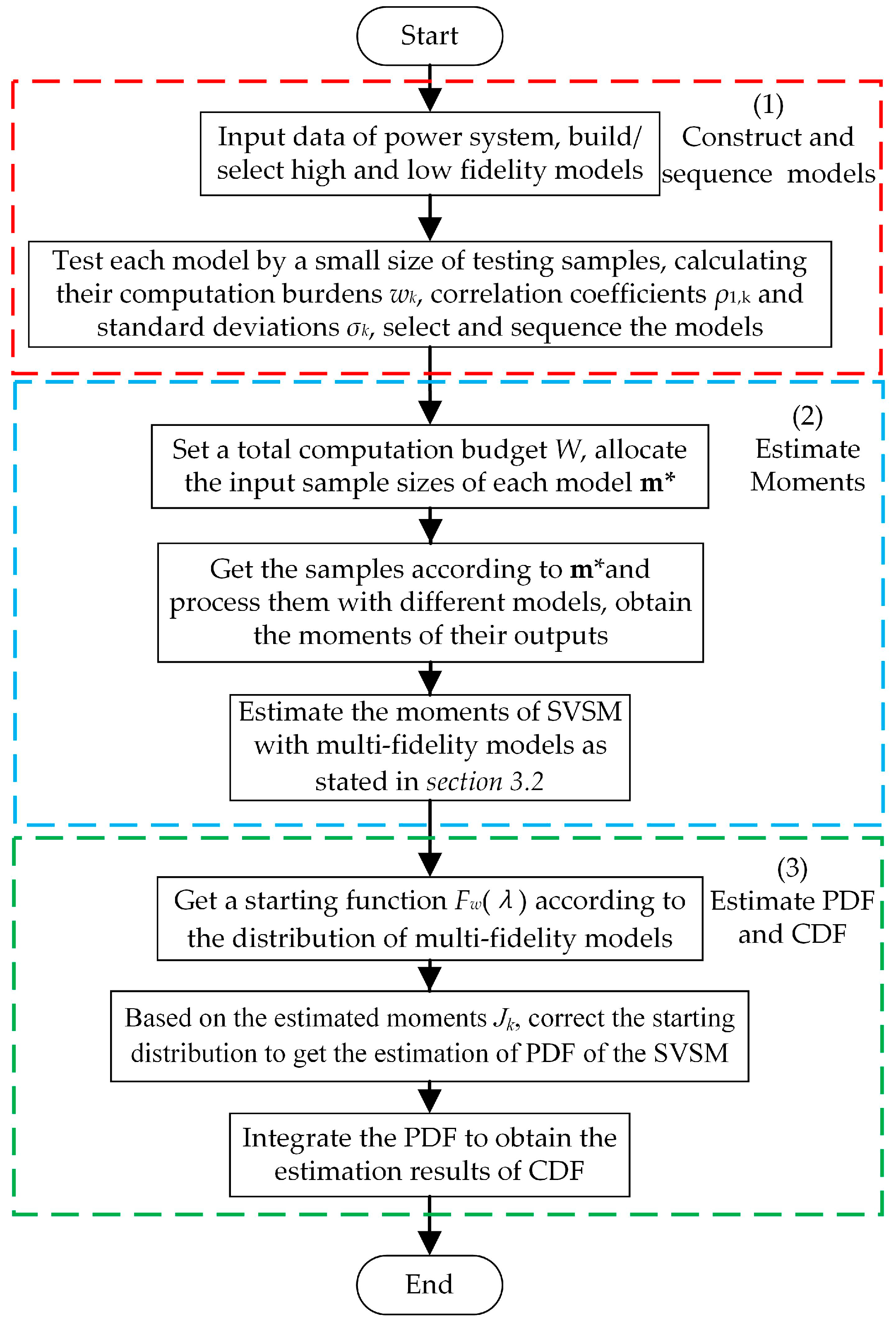
The flowchart of stochastic SVSM calculation based on MFM is shown in Figure 2, with the following specific steps.

• Construct and sequence the high- and low-fidelity models

(1) Construct a high-fidelity model based on the source, load, and line information of the power system. Construct multiple low-fidelity models using different methods, such as simplification and proxy (or choose high- and low-fidelity models from pre-constructed models of the power system being analyzed).

(2) Obtain a small set of test input samples (e.g., sample size of 1000) using the source–load model proposed in Section 2.3. Test the computational burden w_k and standard deviation σ_k of each model by calculating the correlation coefficients ρ_1,k between the outputs of each low-fidelity and high-fidelity model, then select and sequence the models using Equations (14)–(16).

2.

Estimate the moments of the SVSM

(1) Give a total computational budget W, then calculate the sample size sequence m* for each as Equations (17) and (18). The input samples are obtained based on the sample size assigned to each model.

(2) Estimate the moments of SVSM using Equations (12) and (26) the outputs of MFMs.

3.

Estimate the PDF and CDF of the SVSM

(1) Based on the selected high- or low-fidelity model, construct a starting distribution F_w(λ). Calculate the first origin moments D_k (k = 1,2,…,2G) of this starting distribution. Use the origin moments estimated by the MFM method as the first M-order origin moments D′_k (k = 1,2,…) of the real distribution.

(2) Estimate the PDF using Equations (29)–(31). Integrate the resulting PDF to obtain the estimated results of the CDF.

5. Case Studies

5.1. Case Introduction

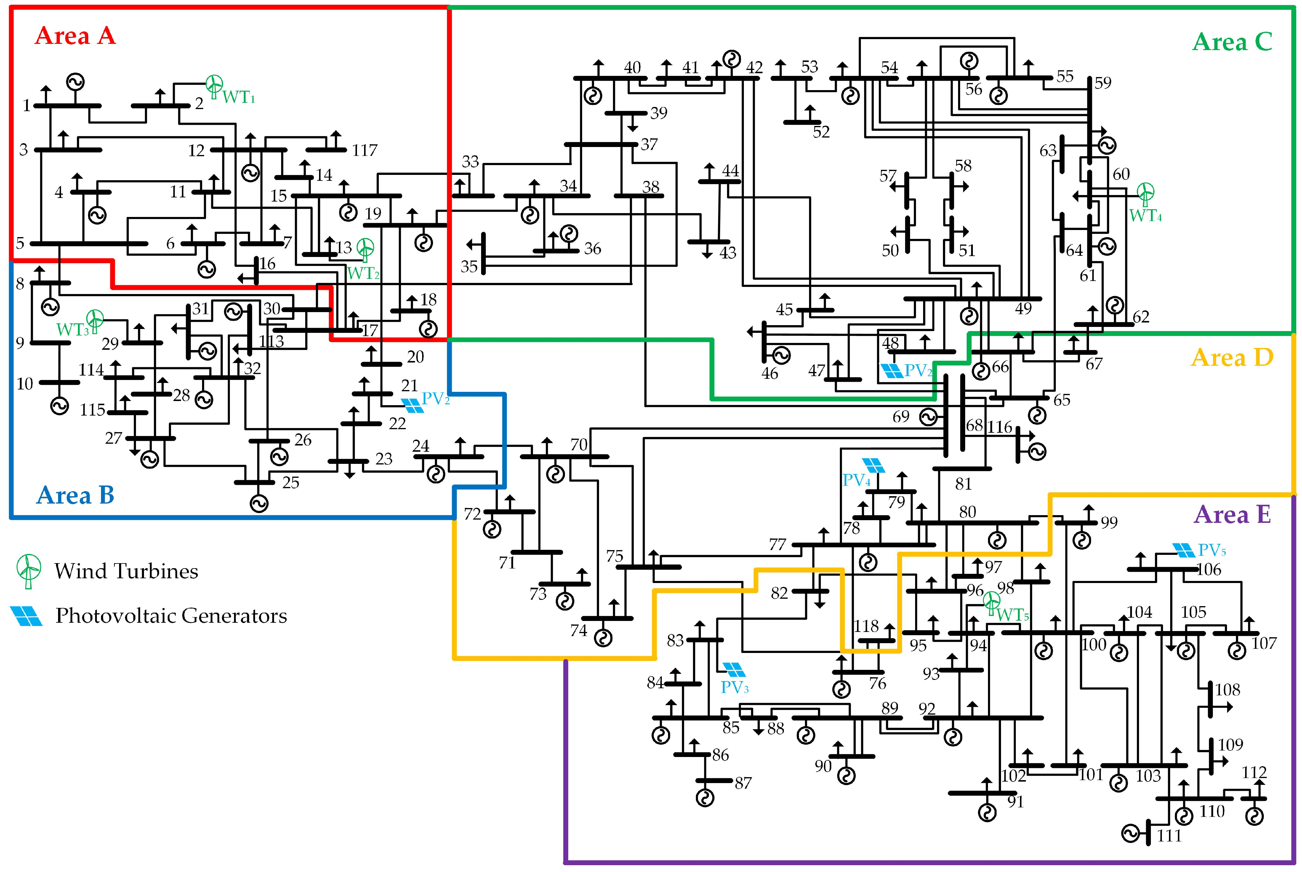
In this work, an IEEE 118-bus transmission grid, as shown in Figure 3, is used to verify the effectiveness of the proposed method. The power system is connected to a total of 10 distributed renewable energy generators (RDGs), including 5 PVGs numbered PV_1~5 and 5 WTs numbered WT_1~5. The parameters of wind speed, solar irradiance, WTs, and PVGs are shown in

Table A1. Parameters of wind speed and wind turbines.

No.	Beta Distribution Parameters		Wind Turbine Parameters
	Shape Parameter	Scale Parameter	vin/ (m/s)	vout/ (m/s)	vN/ (m/s)	PN/ kW
1	3.0	7.5	3.5	20.0	14.5	600
2	2.0	7.0	3.0	19.0	13.0	600
3	2.5	6.0	3.5	20.0	15.5	600
4	2.5	7.5	3.0	18.5	13.0	750
5	3.0	6.0	3.5	19.0	14.0	750

and

Table A2. Parameters of irradiation intensity and photovoltaic cells.

No.	Beta Distribution Parameters		PV Cell Parameters
	ξa	ξb	A/m2	η/%
1	0.40	8.56	25,200	15
2	0.45	9.81	19,800	14
3	0.50	8.94	24,375	16
4	0.40	8.56	25,200	15
5	0.45	9.81	19,800	14

in Appendix A, and the correlation coefficients between the wind speeds and the solar irradiance are assumed to be 0.1 and 0.2, respectively.

In addition to the stochastic output of 10 RDGs, this paper divides the nodes in the distribution network example into five regions (A~E), as seen in Figure 3, and takes the fluctuation amount of the node loads in each region as the input random variable, with the variance set to 1% of the base load; the different regions are independent of each other. Therefore, the example contains a total of 15 input random variables. For this case, the high-fidelity model is the Monte Carlo simulation method (based on the CPF with the original power flow model) [37], the low-fidelity model is the SPCE agent model, and the simplified CPF that only retains the prediction part of the prediction correction algorithm in the CPF. The proposed MFM method is used to characterize the uncertainty of the SVSM. The simulation programs are developed under MATLAB R2023a with a hardware environment of 16GB RAM and Intel core i5-13600 CPU.

5.2. Results of Mean Estimation

5.2.1. Comparison of Accuracy with High-, Low-, and Multi-Fidelity Models

Since the high-fidelity model is assumed to be unbiased, to compare the precision of each model in estimating the moments of SVSM, this paper takes the mean, variance, and higher-order moments of the SVSM of the power system obtained from 1 × 10⁶ CPF calculations as the reference values, and the computational errors are evaluated with the mean square error (MSE) of the multiple calculations. The MSE is defined as follows:

$$\mathrm{MSE}={\displaystyle \frac{1}{Z}}{\displaystyle \sum _{i=1}^Z{\left({\hat{s}}_i-s\right)}^2},$$

(32)

where ${\hat{s}}_i$ is the estimated value of the SVSM from the i-th calculation; s is the true value of the SVSM (or the baseline value); and Z is the total number of estimations.

The input–output samples obtained from 1000 MCSs with the original power flow model are used to establish the SPCE agent model, where the highest order of the SPCE model is set to 4. The high- and low-fidelity models are computed 500 times to obtain their computational burdens, correlation coefficients, means, and variances, as shown in

Table 1. Comparison of computation burden of high-fidelity and low-fidelity models.

Model	Time for 500 Calculations (s)	Computation Burden (Times of MCS)
MCS(CPF)	11.27	1.0000
CPF(Simplified)	5.43	0.4820
SPCE	0.04	0.0043

and

Table 2. Sample sizes for estimating the moments of SVSM with the multi-fidelity model method.

Models	Correlation Coefficients ρ1,k	Mean of Outputs Ek	Variance of Outputs σk2	Input Sample Sizes
MCS(CPF)	1.000000	0.8169392	7.918803 × 10−5	203
CPF(Simplified)	0.999954	0.8239151	7.774890 × 10−5	11,303
SPCE	0.993071	0.8169068	7.998040 × 10−5	1,011,582

. To facilitate the subsequent comparison, the computational burdens are normalized based on the computational burden of the high-fidelity model (i.e., MCS (CPF)), as shown in Table 1. The computational burdens for a single calculation with the CPF(Simplified) and SPCE models are 0.4820 times of MCS and 0.0043 times of MCS, respectively.

Set the total computational budget as 10, 100, 1000, and 10,000 times of MCS. The mean, variance, and higher-order moment estimation of the SVSM are obtained only by the high-fidelity model (MCS(CPF)), the low-fidelity model (Simplified CPF or SPCE agent model), and the proposed MFMs. The allocation of sample sizes inputted into MFMs under the budget of 10,000 MCSs are shown in Table 2. Furthermore, the estimation through high-, low-, and MFMs is repeated 50 times under each given total computational budget to obtain the MSE of the moment estimation (mean E(λ), variance D(λ), fifth-order origin moment J₅(λ), and sixth-order origin moment J₆(λ)). The MSE results are shown in Figure 4 and Figure 5.

As can be seen from Table 2, under the computational budget of 10,000 MCSs, the MFM sequences are ordered by {MCS(CPF), CPF(Simplified), SPCE}. Their correlation coefficients decrease in descending order of ranking (ρ_1,2 > ρ_1,3), while their input sample sizes increase accordingly. A single calculation of CPF(Simplified) is significantly faster than the original CPF, as it retains only the prediction part of the prediction-correction algorithm but not the correct the results by correction. The simplified CPF has a high correlation with the original model but with a large difference in the means, which levels out the estimation results. The same conclusion can be reached under other budgets. The above results indicate that the proposed MFM method can successfully allocate the input samples into each model according to their correlation coefficients and calculating speeds, as well as under the limit of total computational budget.

From the comparison of moment estimation MSEs from different models in Figure 4 and Figure 5, the following conclusions can be drawn.

• With an increasing total computational budget, the gaps between the estimation results and the true moments of λ with high-, low-, and multi-fidelity models all have a decreasing tendency; however, when the given computational budget exceeds a certain value (e.g., 10³ MCSs), the MSEs of the low-fidelity models (CPF(Simplified), SPCE) remain almost unchanged, while the MSEs of the high-fidelity (MCS(CPF)) and MFM estimation results can still continue to decrease as before. This indicates that the low-fidelity model is biased with inherent systematic bias, and its computational accuracy has an upper limit when the calculation number is large enough, while the MFM is able to maintain the same unbiasedness as the high-fidelity model, and the estimation results can keep converging to the benchmark value with the increase in computational budget.
• Compared to using only a high-fidelity model, the proposed MFM method has a smaller MSE (1~2 orders of magnitude accuracy advantage in this case) under the same computational budget, indicating that the proposed method effectively improves computational accuracy while ensuring unbiasedness.
• Compared to the low-fidelity model, the MSE of the computational results of the MFMs is not much different from that of the low-fidelity model when the computational burden is small (e.g., less than 10² MCSs), but as the computational burden increases, the computational accuracy of the MFM will be better than that of the low-fidelity model.
• For variance and higher-order moments, although the optimality of input sample size allocation cannot be guaranteed, the MFM method can also effectively improve the calculation’s accuracy, which is better than that of the high-fidelity model under the same computational burden. This shows the applicability of this sample size allocation to estimating higher-order moments.

Furthermore, we compared the evaluation results obtained from MFM sequence {MCS(CPF), SPCE} with that from {MCS(CPF), CPF(Simplified), SPCE}, and drew their MSE curves at time budgets ranging from 10 to 10,000 times of MCS(CPF) with 50 replicates. Set ${\sigma }_1^2$/W = 1, the optimization coefficient v_j derived using Equation (16) for the MFM sequences {MCS(CPF), SPCE} and {MCS(CPF), CPF(Simplified), SPCE} are 0.0334 and 0.0224, respectively. The optimization coefficient of the MFM sequence with three models is smaller, predicting that this sequence will have the better evaluation stability. The results are shown in Figure 6, and the following conclusions can be drawn.

• Both of the MSE curves of MFM method with different MFM sequences are under the curve of the high-fidelity model (MCS(CPF)), indicating that introducing low-fidelity models can effectively increase the computation stability of the SVSM evaluation with the proposed method.
• The MSE curve of the MFM sequence with two models is almost above that of three models, meaning that the SVSM evaluation stability becomes better with an additional low-fidelity model (CPF(Simplified)), which is consistent with the previous predictions using Equation (16).

This indicates that adding low-fidelity models after the proposed prediction method as Equation (16) can effectively accelerate the calculation of the stochastic SVSM evaluation while maintaining the same accuracy as that of the high-fidelity model.

In summary, the MFM method can effectively improve the accuracy of the moment estimation results while ensuring its unbiasedness.

5.2.2. Comparison of Stability with High-, Low-, and Multi-Fidelity Models

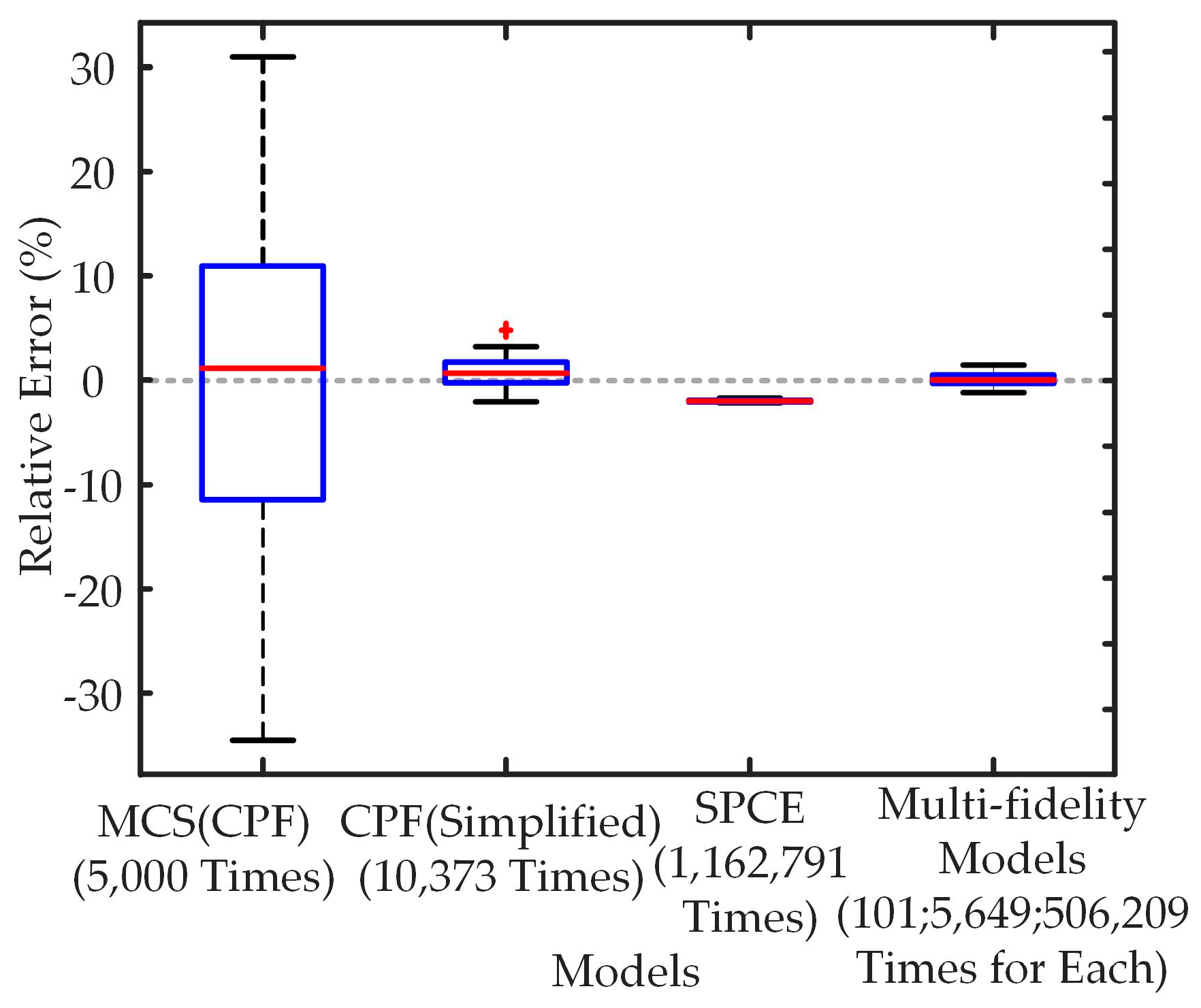
In order to compare the stability of different methods, this paper estimates the SVSM under a given total computational budget of 5000 MCSs, repeats it 50 times using the high-, low-, and multi-fidelity models, respectively, and finally calculates the relative errors between the results and the benchmark value. The boxplot of the error distributions is shown in Figure 6. The following conclusions can be drawn from Figure 7.

• The errors of both the MFM and the high-fidelity model (MCS(CPF)) fluctuate around 0, but the fluctuation range of the error distribution of the MFM is smaller in comparison; this indicates that although both are unbiased estimators, the error fluctuation of the results obtained from the MFMs is smaller and the stability of this method is better.
• The error distribution of the low-fidelity model (especially SPCE) is concentrated, but the range of its distribution is somewhat different from 0; this indicates that there is an inherent systematic bias in the computation of the low-fidelity models, and their accuracy cannot be guaranteed by increasing the calculation number, even though if results are very stable.

5.3. Results of the Probabilistic Distribution Estimation

To estimate the PDF and CDF of SVSM, the MFMs are constructed under a computational budget of 1000 MCSs to obtain the starting distribution and high-order moments required in Section 2.2. The estimated distribution is then compared with that from each single model under the computational budget of 1000 MCSs (MCS(CPF): 1000 times, CPF(Simplified): 2075 times, SPCE: 232,558 times) and that from the level expansion methods, based on the moments obtained from the MFM method, to validate the efficiency of the proposed method.

In this case, we use the output statistics of the SPCE agent model during the MFM computation as the starting distribution (because it is assigned more samples to generate outputs, whose distributions are stable and close to the original model), and the highest order is set to G = 6. The first six orders of the origin moments of the SVSM obtained from the MFM method are shown in

Table 3. Estimation results for the first sixth-order origin moments of λ.

Order of Origin Moment k	Jk(λ)	Order of Origin Moment k	Jk(λ)
1	0.8169	4	0.4457
2	0.6675	5	0.3643
3	0.5454	6	0.2978

.

• Comparison of the estimation results from single the model and the proposed method

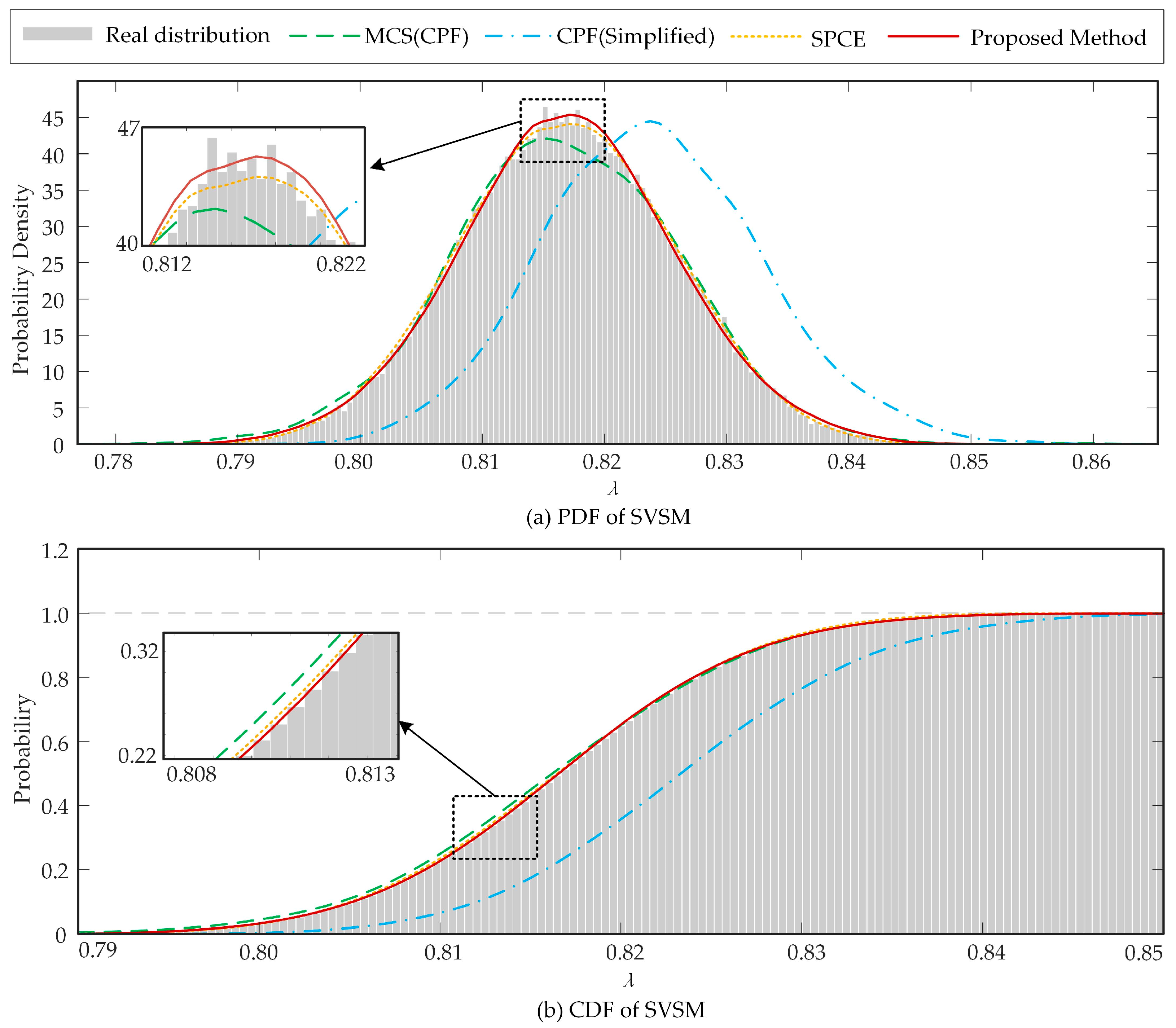
To compare the estimation results from the single model with that from MFMs based on the correction method of the starting distribution, we calculate the probabilistic distribution of SVSM using the starting distribution method according to Equation (30), and then analyze the output of each single model to obtain the PDF results from only high- and low-fidelity models. Finally, the PDFs are integrated to obtain the CDFs. The results are shown in Figure 8. It is assumed that the SVSM obtained from 1 × 10⁶ times of the MCS (CPF) serves as the actual distribution benchmark.

As can be seen in Figure 8, the PDF and CDF obtained by the proposed method match the most closely with the actual distribution, while other single-model computation results have some deviations, especially at the peak (with x-label 0.81~0.82). Among them, the result from MCS (CPF) has a large discrepancy with the actual distribution due to its small number of calculations (1000 times); CPF(Simplified) even has a larger error in the horizontal coordinate of the distribution because it is equivalent to a translation of the results. The SPCE method has the largest number of calculations (232,558 times), but due to the inherent error between the proxy model and the original model, it cannot completely approximate the actual distribution. The proposed method, on the other hand, takes SPCE as the starting distribution and corrects it with the high-precision moments obtained from the MFM method, effectively improving the estimation accuracy of the PDF of SVSM.

2.

Comparison of the estimation results of the level expansion methods and the proposed method

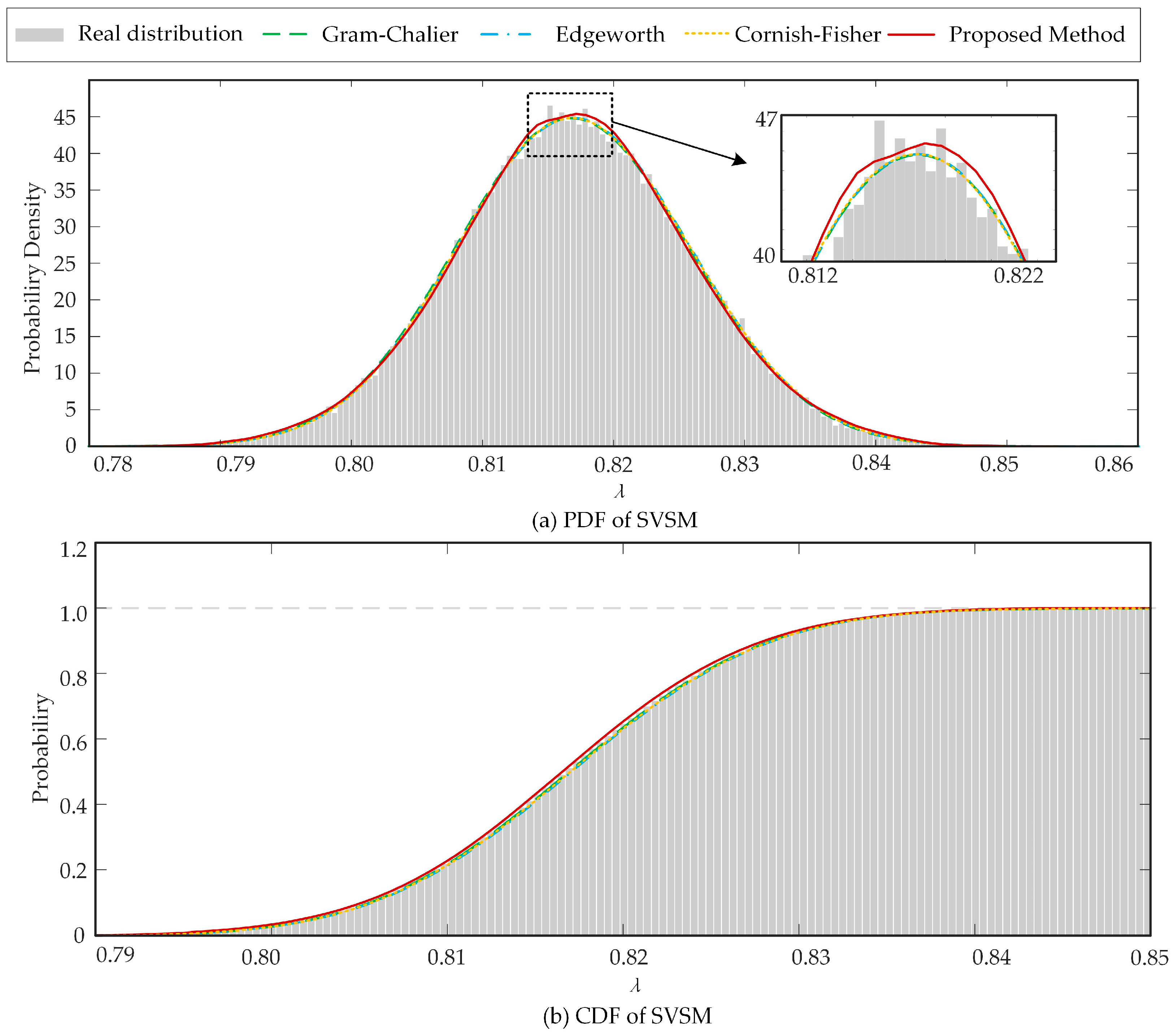
Based on the high-order moments estimated through the MFM method, the PDF and CDF of SVSM are then estimated by the Gram–Chalier expansion, Edgeworth expansion, and Cornish–Fisher expansion, and finally compared with the proposed method. As can be seen in Figure 9, the results obtained by the three-level expansion methods are very close to each other, but the estimation results are all slightly worse than the proposed method, especially at the peaks (with x-label 0.81~0.82). This is due to the fact that the distribution of SVSM is close to the normal distribution, and thus the level expansion methods are effective; but since they only use the moments without the distribution of the model output, their accuracy is inferior to that of the proposed method. The proposed method, on the other hand, can make better use of all the prior information obtained from the estimation of the moments with the MFM method, and, therefore, has a higher accuracy.

6. Conclusions

In this paper, we proposed a method for characterizing the stochastic SVSM of a power system with a high percentage of renewable energy based on MFMs. This method can work well according to a pre-given total computational budget, as it combines the advantages of high- and low-fidelity models and reasonably allocates the number of input samples to achieve high-precision estimation of the moments, PDF, and CDF of the SVSM. The main conclusions are as follows.

• Compared to the high-fidelity model (MCS, in the studied case), the proposed MFM method can keep 1~2 orders of magnitude accuracy advantage over the high-fidelity model at the MSE of SVSM moment evaluation, while keeping the same MSE descending speed as the high-fidelity model when the computational budget increases. This indicates that this method can compensate for the efficiency and accuracy of the calculation of stochastic SVSM and obtain the SVSM moment evaluation results with the same accuracy as the high-fidelity model, while accelerating the computation speed with the low-fidelity models.
• Compared to the low-fidelity models (CPF(Simplified), SPCE), the proposed MFM method exhibits sustained MSE reduction proportional to increased computational budget allocation. This diverges fundamentally from low-fidelity approaches that encounter inherent accuracy ceilings due to structural limitations. The persistent convergence behavior demonstrates the method’s statistical consistency and numerical stability, enabling superior moment estimation accuracy for stochastic SVSM compared to standalone low-fidelity models.
• For the estimation of PDF and CDF of SVSM, under constrained computational budgets (1000 MCS equivalent evaluations), the proposed startup function-based fitting method outperforms both individual models (high- and low-fidelity) and conventional-level expansion techniques in PDF/CDF reconstruction, with the benchmark derived from many more evaluations of the high-fidelity model (106 MCS evaluations). This indicates that the proposed method can fit the SVSM distribution better with a lower computational budget than the other investigated methods, while achieving performance similar to the high-fidelity model for large sample evaluations.

References

1. Yun, Z.; Cui, X. Online preventive control method for static voltage stability of large power grids. IEEE Trans. Power Syst. 2020, 35, 4689–4698. [Google Scholar]
2. Fan, Y.; Liu, S.; Qin, L.; Li, H.; Qiu, H. A novel online estimation scheme for static voltage stability margin based on relationships exploration in a large data set. IEEE Trans. Power Syst. 2014, 30, 1380–1393. [Google Scholar]
3. Wang, Q.; Lin, S.; Yang, Y.; Liu, M. A decomposition and coordination algorithm for SVSM interval of integrated transmission and distribution networks considering the uncertainty of renewable energy. Int. J. Electr. Power Energy Syst. 2022, 136, 107761. [Google Scholar]
4. Van Cutsem, T.; Vournas, C. Voltage Stability of Electric Power Systems, 1st ed.; Kluwer Academic Publishers: Dordrecht, The Netherlands, 1998; p. 188. [Google Scholar]
5. Rodrigues, A.B.; Prada, R.B.; da Silva, M.D.G. Voltage stability probabilistic assessment in composite systems: Modeling unsolvability and controllability loss. IEEE Trans. Power Syst. 2010, 25, 1575–1588. [Google Scholar]
6. Liu, K.Y.; Sheng, W.; Hu, L.; Liu, Y.; Meng, X.; Jia, D. Simplified probabilistic voltage stability evaluation considering variable renewable distributed generation in distribution systems. IET Gener. Transm. Distrib. 2015, 9, 1464–1473. [Google Scholar]
7. Xie, Y.; Lin, S.; Liang, W.; Yang, Y. Interval Probabilistic Energy Flow Calculation of CCHP Campus Microgrid Considering Interval Uncertainties of Distribution Parameters. IEEE Access 2020, 8, 141358–141372. [Google Scholar]
8. Kiefer, J. On large deviations of the empiric DF of vector chance variables and a law of the iterated logarithm. Pacific J. Math. 1961, 11, 649–660. [Google Scholar] [CrossRef]
9. Yu, H.; Chung, C.Y.; Wong, K.P.; Lee, H.W.; Zhang, J.H. Probabilistic load flow evaluation with hybrid latin hypercube sampling and cholesky decomposition. IEEE Trans. Power Syst. 2009, 24, 661–667. [Google Scholar]
10. Bratley, P.; Fox, B.L. Algorithm 659: Implementing Sobol’s quasirandom sequence generator. ACM Trans. Math. Softw. (TOMS) 1988, 14, 88–100. [Google Scholar]
11. Saunders, C.S. Point estimate method addressing correlated wind power for probabilistic optimal power flow. IEEE Trans. Power Syst. 2013, 29, 1045–1054. [Google Scholar]
12. Zhang, P.; Lee, S.T. Probabilistic load flow computation using the method of combined cumulants and Gram-Charlier expansion. IEEE Trans. Power Syst. 2004, 19, 676–682. [Google Scholar]
13. Moreira, E.; Chagas, E.; Rodrigues, A.; da Silva, M.D.G. Linear probabilistic power flow for islanded microgrids. In Proceedings of the 2020 International Conference on Probabilistic Methods Applied to Power Systems (PMAPS), Liege, Belgium, 18–21 August 2020; IEEE: New York, NY, USA; pp. 1–6. [Google Scholar]
14. Jiang, Y.; Ren, Z.; Sun, Z.; Li, W.; Yang, X. A stochastic response surface method based probabilistic energy flow analysis method for integrated electricity and gas systems. IEEE Trans. Power Syst. 2022, 37, 2467–2470. [Google Scholar]
15. Ni, F.; Nguyen, P.H.; Cobben, J.F. Basis-adaptive sparse polynomial chaos expansion for probabilistic power flow. IEEE Trans. Power Syst. 2016, 32, 694–704. [Google Scholar]
16. Wu, H.; Zhou, Y.; Dong, S.; Xin, H.; Song, Y. Probabilistic load flow by generalized polynomial chaos method. In Proceedings of the 2016 IEEE Power and Energy Society General Meeting (PESGM), Boston, MA, USA, 17–21 July 2016; IEEE: New York, NY, USA; pp. 1–5. [Google Scholar]
17. Aien, M.; Fotuhi-Firuzabad, M.; Aminifar, F. Probabilistic load flow in correlated uncertain environment using unscented transformation. IEEE Trans. Power Syst. 2012, 27, 2233–2241. [Google Scholar]
18. Wu, H.; Zhou, Y.; Dong, S.; Song, Y. Probabilistic load flow based on generalized polynomial chaos. IEEE Trans. Power Syst. 2016, 32, 820–821. [Google Scholar]
19. Amid, P.; Crawford, C. A cumulant-tensor-based probabilistic load flow method. IEEE Trans. Power Syst. 2018, 33, 5648–5656. [Google Scholar]
20. Khatami, R.; Parvania, M. Stochastic multi-fidelity scheduling of flexibility reserve for energy storage. IEEE Trans. Sustain. Energy 2020, 11, 1438–1450. [Google Scholar]
21. Zhang, Y.; Li, Y.; Qiu, F.; Hong, T.; Markel, L. Learning frequency nadir from multi-fidelity data for dynamic secure microgrid islanding. In Proceedings of the 2022 IEEE Power & Energy Society General Meeting (PESGM), Denver, CO, USA, 17–21 July 2022; pp. 1–5. [Google Scholar]
22. Zhu, B.; Ren, S.; Wei, Z.; Si, F. Transfer learning-based multi-fidelity modeling method for multimode process monitoring. In Proceedings of the 2024 IEEE 4th International Conference on Digital Twins and Parallel Intelligence (DTPI), Wuhan, China, 18–20 October 2024; pp. 465–470. [Google Scholar]
23. Yang, S.; Vaagensmith, B.; Patra, D.; Hruska, R.; Phillips, T. Multi-fidelity power flow solver. In Proceedings of the 2022 Resilience Week (RWS), National Harbor, MD, USA, 26–29 September 2022; pp. 1–6. [Google Scholar]
24. Ye, K.; Pei, Y.; Zhao, J.; Yao, Y.; Wang, J.; Ding, F. Multi-fidelity learning for distribution system voltage probabilistic analysis with high penetration of PVs. In Proceedings of the 2022 IEEE Power & Energy Society General Meeting (PESGM), Denver, CO, USA, 17–21 July 2022; pp. 1–5. [Google Scholar]
25. Ajjarapu, V.; Christy, C. The continuation power flow: A tool for steady state voltage stability analysis. IEEE Trans. Power Syst. 1992, 7, 416–423. [Google Scholar]
26. Xu, X.; Yan, Z.; Shahidehpour, M.; Wang, H.; Chen, S. Power system voltage stability evaluation considering renewable energy with correlated variabilities. IEEE Trans. Power Syst. 2017, 33, 3236–3245. [Google Scholar]
27. Chen, Y.; Wen, J.; Cheng, S. Probabilistic load flow method based on Nataf transformation and Latin hypercube sampling. IEEE Trans. Sustain. Energy 2012, 4, 294–301. [Google Scholar]
28. Fan, M.; Li, Z.; Ding, T.; Huang, L.; Dong, F.; Ren, Z.; Liu, C. Uncertainty evaluation algorithm in power system dynamic analysis with correlated renewable energy sources. IEEE Trans. Power Syst. 2021, 36, 5602–5611. [Google Scholar] [CrossRef]
29. Bay, Y.D.; Suvorov, A.A.; Gusev, A.S.; Razzhivin, I.A.; Askarov, A.B. Stochastic modeling of a DFIG wind turbine in Matpower. IEEE Access 2021, 9, 76005–76014. [Google Scholar] [CrossRef]
30. Obadina, O.O.; Berg, G.J. Determination of voltage stability limit in multimachine power systems. IEEE Trans. Power Syst. 1988, 3, 1545–1554. [Google Scholar] [CrossRef]
31. Canizares, C.A.; Alvarado, F.L. Point of collapse and continuation methods for large AC/DC systems. IEEE Trans. Power Syst. 1993, 8, 1–8. [Google Scholar] [CrossRef]
32. Villanueva, D.; Pazos, J.L.; Feijoo, A. Probabilistic load flow including wind power generation. IEEE Trans. Power Syst. 2011, 26, 1659–1667. [Google Scholar] [CrossRef]
33. Peherstorfer, B.; Willcox, K.; Gunzburger, M. Optimal model management for multifidelity Monte Carlo estimation. SIAM J. Sci. Comput. 2016, 38, A3163–A3194. [Google Scholar] [CrossRef]
34. Qian, E.; Peherstorfer, B.; O’Malley, D.; Vesselinov, V.V.; Willcox, K. Multifidelity Monte Carlo estimation of variance and sensitivity indices. SIAM/ASA J. Uncertain. Quantif. 2018, 6, 683–706. [Google Scholar] [CrossRef]
35. Fan, M.; Vittal, V.; Heydt, G.T.; Ayyanar, R. Probabilistic power flow studies for transmission systems with photovoltaic generation using cumulants. IEEE Trans. Power Syst. 2012, 27, 2251–2261. [Google Scholar] [CrossRef]
36. Tekel, J.; Cohen, L. Constructing and estimating probability distributions from moments. In Proceedings of the Automatic Target Recognition XXII, Baltimore, MD, USA, 23–24 April 2012; SPIE: Bellingham, WA, USA; Volume 8391, pp. 114–123. [Google Scholar]
37. Li, S.H.; Chiang, H.D. Nonlinear predictors and hybrid corrector for fast continuation power flow. IET Gener. Transm. Distrib. 2008, 2, 341–354. [Google Scholar] [CrossRef]
Figure 1. Schematic of computation efficiency and accuracy of high- and low-fidelity models.
Energies 18 01614 g001
Figure 2. Flow Chart of the Stochastic SVSM Analysis Method Using the Multi-Fidelity Models.
Energies 18 01614 g002
Figure 3. IEEE 118-bus Power System with RDGs.
Energies 18 01614 g003
Figure 4. Results of MSE for E(λ) and D(λ) under different computation budgets.
Energies 18 01614 g004
Figure 5. Results of MSE for J5(λ) and J6(λ) under different computation budgets.
Energies 18 01614 g005
Figure 6. Results of MSE for E(λ) and D(λ) under different MFM sequences.
Energies 18 01614 g006
Figure 7. Boxplot of the relative errors of the variance estimation of SVSM.
Energies 18 01614 g007
Figure 8. Fitting results for the PDF and CDF of SVSM with different models.
Energies 18 01614 g008
Figure 9. Fitting results for the PDF and CDF of SVSM with level expansion methods and the proposed method.
Energies 18 01614 g009