Grey-Box Modelling of District Heating Networks Using Modified LPV Models

Abstract

The International Energy Agency (IEA) 2023 report highlights that global energy losses have persisted over the years, with 32% of the energy supply lost in 2022 alone. To mitigate this, this research adopts optimisation to enhance the efficiency of district heating networks (DHNs), a key global energy supply technology. Given the dynamic nature of DHNs and the challenges in predicting disturbances, a dynamic real-time optimisation (DRTO) approach is proposed. However, this research does not implement DRTO; instead, it develops a fast grey-box linear parameter varying (LPV) model for future integration into the DRTO algorithm. A high-fidelity physical model replicating theoretical time delays in pipes serves as a reference for model validation. For a single pipe, the grey-box model achieved a 91.5% fit with an $R^2$ value of 0.993 and operated 5 times faster than the reference model. At the DHN scale, it captured 98.64% of the reference model’s dynamics, corresponding to an $R^2$ value of 0.9997, while operating 52 times faster. Low-fidelity physical models (LFPMs) were also developed and validated, proving to be more precise and faster than the grey-box models. This research recommends performing dynamic optimisation with both models to determine which better identifies local minima.

1. Introduction

1.1. Background of the Study

The International Energy Agency (IEA) 2023 report indicates that, since 1990, more energy has consistently been supplied to compensate for the energy losses [1]. As a result, an average of approximately 31% of the global energy supplied has been lost over the years [1]. Thus, the IEA 2023 report highlights energy efficiency enhancement as one of the key strategies for reducing global energy waste [1]. Among the various sectors using the global energy supply, approximately 50% is allocated to thermal energy generation (TEG) [1]. Therefore, improving the efficiency of the thermal energy generation sector can significantly enhance the global energy supply efficiency and reduce global energy losses. Research has shown that optimisation effectively improves efficiency [2]. Consequently, this research focuses on developing a methodology for optimising the district heating networks (DHNs) of the global thermal energy generation sector to improve the global energy supply efficiency and contribute to global energy and environmental sustainability. A district heating network (DHN) generates energy in a central station and distributes it to consumers according to their dynamically changing power demands [3]. So, the operation of a DHN is dynamic, demanding the implementation of dynamic optimisation. Also, this network operation is influenced by unpredictable meteorological conditions [4], which are best forecasted in the short term (real time). Consequently, this paper is the first phase of the research, which aims to perform the dynamic real-time optimisation of a DHN to enhance the network efficiency.

A dynamic real-time optimisation (DRTO) algorithm performs repetitive sequential optimisations based on updated system disturbances and current state conditions [5,6]. This approach requires low-computation models to allow frequent optimisations as disturbances are predicted [7,8]. Models are broadly categorised into three types: physical (white box), black box, and grey box [9]. The physical models are high-order detailed models with high precision but are computationally expensive [9]. Thus, they may be unsuitable for real-time operation [10], particularly for complex physical systems with intricate models. Black-box models, which are based on historical data, suffer from low extrapolation capability [11]. This extrapolation capacity is indispensable for optimisation algorithms, so this research does not consider black-box models. In contrast, the grey-box models have good interpolation capability because they blend physical model structures with data, offering a balance of speed and reliability [12]. Moreover, grey-box models make it possible to estimate hidden states, which can be employed for other predictions [13]. Hence, this paper proposes a grey-box model for DHNs. While no optimisation is implemented here, the proposed grey-box model can serve as a foundation for facilitating real-time DHN optimisation. Nevertheless, the grey-box model is validated with the simulation result of a nonlinear physical DHN model to ensure its compatibility with the network operation. Thus, the principal objectives of this research are the physical and grey-box modelling of a DHN as well as the validation of the grey-box model.

1.2. Literature Review on Grey-Box Models

Several grey-box models can be formulated from the physics of a system. The research study by [10] proposed a grey-box model to estimate the hydraulic parameters of a tree-shaped DHN, aiming to ameliorate pumping efficiency during network control. In conventional DHN modelling, the hydraulic model relies on the pressure losses within the network pipes [14]. However, the research of [10] developed a grey-box hydraulic model that depends solely on the pressure measurements at two consumer substations in the network [10]. The hydraulic model is then validated through a case study simulation of a DHN, achieving an estimation measurement error of less than 1%.

A common grey-box model for thermal systems adopts the resistance-capacitance (RC) circuit analogy from electrical systems to define its structure [15]. This modelling principle is called the RC modelling [15]. The model parameters are the resistances and capacitances of the circuit, which can be identified through system identification techniques [15]. The research study by [16] developed a nonlinear grey-box model to capture the heat dynamics of a building, enabling predictions of indoor air temperature, return water temperature, and heat load. In this setup, the building receives heat from a district heating network and distributes it to its rooms via radiators. The room modelling process is divided into stages. First, a state-space model structure is formulated from an RC circuit representation of a room, expressing indoor temperature as a function of heat load. Second, an RC circuit representation is developed for the radiators in the room. These two models are then combined to derive a generalised model structure for predicting the building heat dynamics. Given the potential uncertainty in predicting building heat dynamics [16], process and measurement noises with Gaussian densities are incorporated into the deterministic model (the generalised model structure), transforming it into a stochastic nonlinear state space model. Consequently, maximum likelihood, combined with a continuous discrete extended Kalman filter (CDEKF), is employed to identify the model parameters. The research concluded that the nonlinear grey-box model accurately predicted the indoor air temperature, return temperature, and heat load. The stochastic differential equation (SDE) used in this research was similarly developed by [13] to model the heat dynamics of a solar thermal collector. Maximum likelihood was also employed to estimate the grey-box model parameters. The research concluded that the grey-box model agreed with the EN 12975 Quasi Dynamic Test Method (CEN, European Committee for Standardisation, 2006) modelling of the same collector. This validated grey-box model was then employed in the research work of [17] to perform a nonlinear predictive control of a solar thermal system in a district heating system.

The RC modelling principle was also employed in the research work of [18] to develop a grey-box model. This grey-box model, represented by stochastic differential equations, was employed for real-time forecasting and prediction of the transformer temperatures in a power distribution network. This grey-box model accurately predicted the transformer temperatures with a mean absolute error ranging from 0.4 to 0.6 °C.

However, the main challenge in grey-box model development lies in identifying the best model structure that effectively captures the system dynamics at a low computation cost. This challenge can be addressed by explicitly capturing the nonlinear dynamics using linear parameter varying (LPV) modelling techniques [19].

A linear parameter varying (LPV) model is a linear model whose behaviour depends on time-varying parameters called the scheduling parameters or variables [20]. The research study by [19] developed a continuous-time LPV model to predict the outlet temperature of a cross-flow heat exchanger. In this model, the outlet temperature is influenced by the input (inlet temperature) and the scheduling variable (mass flow rate). The LPV model structure is formulated such that the outlet temperature depends on the inlet temperature and the model parameters, while the model parameters are functions of the scheduling variable (mass flow rate). To develop and validate this LPV model, three principal datasets were generated from the simulations of the heat exchanger physical model. The first dataset was used to train the LPV model, identifying both the model parameters and their dependency on the mass flow rate. Initial validation with the second dataset, which had constant mass flow rates, demonstrated over 90% accuracy. However, during the validation with the third dataset, which consisted of continuous mass flow rate profiles, the LPV model failed to capture the system dynamics accurately. To address this limitation, a quasi-LPV model was introduced by modifying the model structure to incorporate additional constant model parameters. This refined model expressed the heat exchanger outlet temperature as a function of the inlet temperature, mass flow rate, and both varying and constant model parameters, and it was validated against the third dataset, achieving 91.56% accuracy. Similar research was conducted by [20] to identify an LPV model that captures the dynamics of a counter-flow water-to-oil heat exchanger. The LPV model is termed a Multiple Input Single Output (MISO) quasi-LPV model [20], and it effectively models the dynamics of the oil heat exchanger under the simultaneous excitation of the inlet temperatures and mass flow rates of both water and oil.

Furthermore, LPV models have been integrated into optimisation and control algorithms to leverage their speed and reliability [21]. The research work of [21] developed a grey-box linear parameter varying (LPV) model to capture the dynamics of a gas-lift system. The model was incorporated into a nonlinear model predictive control (NMPC) algorithm and compared with a physical model-based NMPC algorithm. The results showed that the LPV-based NMPC was three times faster than its physical model counterpart. In addition, the research study by [22] developed an LPV model that can be integrated into an optimisation algorithm for the optimal design of wastewater treatment plants. In this LPV modelling approach, the scheduling variables include the water and air flow rates as well as ammonium concentration. To address the local minima convergence challenge in the optimisation algorithm, a new initialisation strategy (reinitialised partial moment (RPM) filter)) was employed. The LPV model parameters were then identified through the optimisation process and subsequently validated, achieving a 65.45% fit.

1.3. Research Contributions and Novelty

Different classes of grey-box models have been developed in previous research, including the RC and the LPV modelling approaches. Some studies have incorporated process and measurement noises into deterministic models to account for system uncertainty. The research work of [23] applies the Calinski–Harabasz index to address the uncertainty in renewable energy systems, particularly their intermittency challenges. Nevertheless, uncertainty is beyond the scope of this paper. Instead, the proposed LPV grey-box model is directly validated against the simulation results of a DHN physical model.

Furthermore, while some studies have developed grey-box models for the hydraulic modelling of DHNs, to the best of our knowledge, no published research has proposed a methodology for the thermal modelling of DHNs using a modified linear parameter varying (LPV) model. Therefore, this study introduces a novel methodology for LPV-based thermal modelling of DHNs.

In contrast to the RC modelling techniques, where sizing parameters may be lost during model formulation, the proposed LPV model preserves the network sizing parameters to facilitate future DHN design optimisation. In addition, the LPV model is developed under stringent conditions to ensure robustness and computational efficiency, particularly in handling discontinuous input variables. Such discontinuities may arise from emergency system shutdowns.

1.4. Research Objectives and Scope

The objectives of this paper are to develop a physical model of a district heating network, create a grey-box model using LPV techniques, and validate the grey-box model against simulation results for both a single DHN pipe and the entire network. The scope of the paper is outlined as follows: Section 2 discusses the DHN process description, physical modelling, and grey-box model development. Section 3 presents the validation of the grey-box model and provides a discussion of the results. Finally, Section 4 concludes with insights on incorporating the grey-box model into future dynamic real-time optimisation of DHNs.

2. System Description and Modelling

A DHN consists of two main sections: energy generation (production) and distribution. Thermal energy in the form of hot water is generated at a central heat generation station and distributed through insulated pipes to multiple consumers based on their dynamically changing power demands, as depicted in Figure 1.

The production section begins with the main production pipe $pmp$, which directly connects to the generation station and transports hot water to the production splitter. The production splitter then distributes the hot water to branch inlets according to their designated mass flow rates.

The distribution section consists of $nb$ branches, each containing $n{c}_b$ consumer components. Each consumer component has a main pipe that receives hot water and a splitter that diverts a portion of it through an extended-in pipe (also called a lateral-in pipe) $e{p}_{in}$ to its substation to satisfy the consumer’s demand. The remaining hot water continues to the next consumer component via the main pipe. After fulfilling the consumer’s demand, the water cools and exits through an extended-out pipe (lateral-out) $e{p}_{out}$ into the return pipe $rp$. This return pipe channels the cooled water to the consumer mixer, where it mixes with the branch return flow. The mixed return flows from all the branches are mixed in the production mixer before being returned to the heat-generation station via the production return pipe $prp$.

The subsequent section presents the physical and grey-box modelling of both the generation and distribution sections of a DHN.

2.1. Physical Modelling of the Generation Section

As described, the generation section comprises the production splitter, production mixer, the heat-generation station with power $P_{gen}\left(t\right)$, the production main pipe $pmp$, and the production return pipe $prp$, as depicted in Figure 2. The modelling of the production pipes is addressed in Section 2.2. The physical model is developed by applying the principle of mass and energy balance to the components of the DHN.

Production splitter model:

$$\mathrm{Mass} \mathrm{balance} {\dot{m}}_{pmp}\left(t\right)={{\displaystyle \sum }}_b^{nb}{\dot{m}}_{b,c1,mp}\left(t\right)$$

(1)

$$\mathrm{Temperature} \mathrm{equality} T_{pmp,f}\left(t\right)=T_{\mathrm{b},c1,mp,0}\left(t\right) \forall b$$

(2)

Production mixer model:

$$\mathrm{Mass} \mathrm{balance} {\dot{m}}_{prp}\left(t\right)={{\displaystyle \sum }}_b^{nb}{\dot{m}}_{b,c1,rp}\left(t\right)$$

(3)

$$\mathrm{Energy} \mathrm{balance} T_{prp,0 }\left(t\right)={\displaystyle \frac{{{\displaystyle \sum }}_b^{nb}{\dot{m}}_{b,c1,rp}\left(t\right)T_{b,c1,rp,f}\left(t\right)}{{\dot{m}}_{prp}\left(t\right)}}$$

(4)

Equation $\left(4\right)$ assumes that the specific heat capacity of liquid water varies slowly with temperature [24]. Consequently, it is treated as constant in the modelling process. Additionally, it is considered constant for all the mixer models in this paper.

Combined heat-generation station:

$$\mathrm{Energy} \mathrm{balance} P_{gen}\left(t\right)={\dot{m}}_{pmp}\left(t\right)c_p(T_{pmp,0}\left(t\right)-T_{prp,f}\left(t\right))$$

(5)

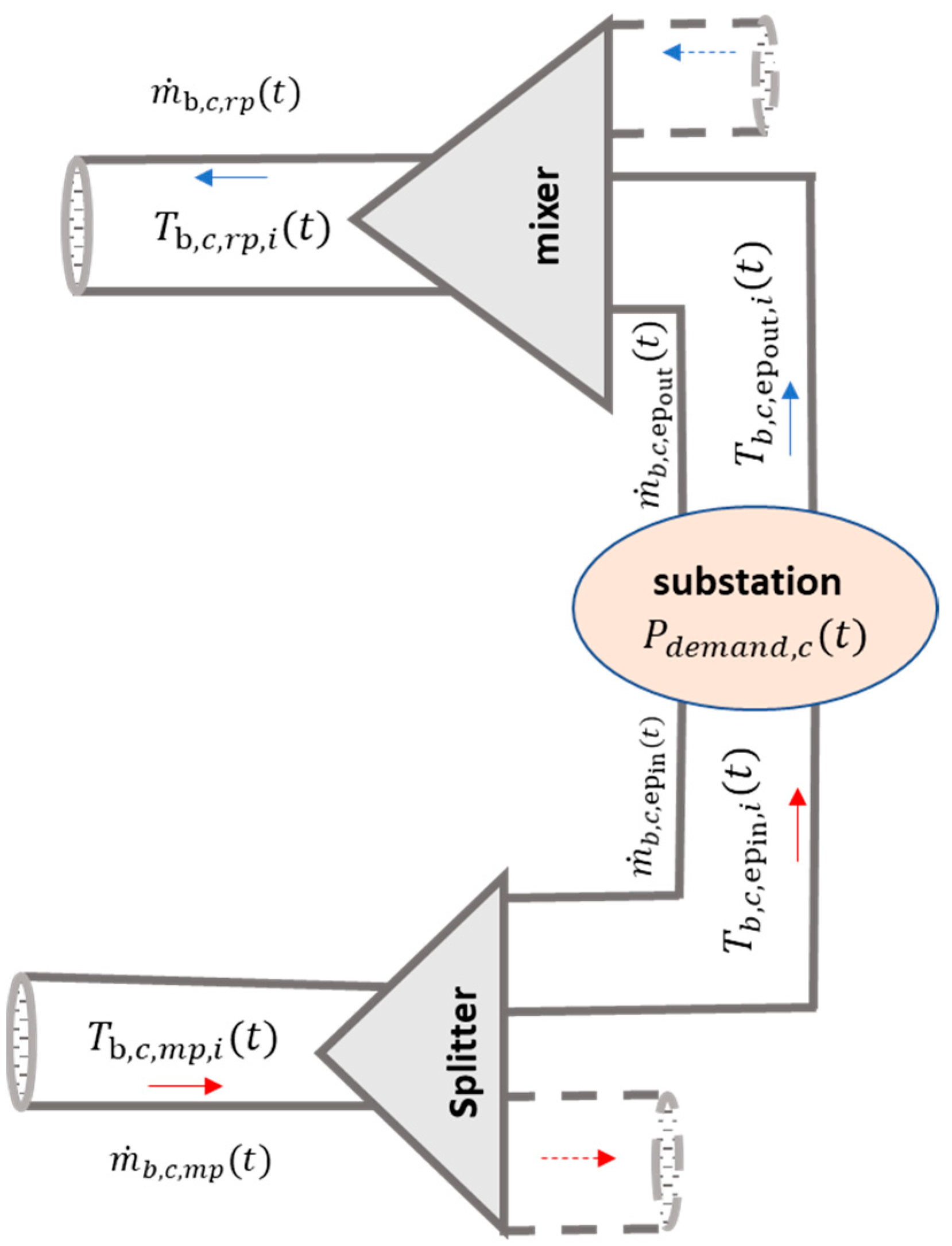
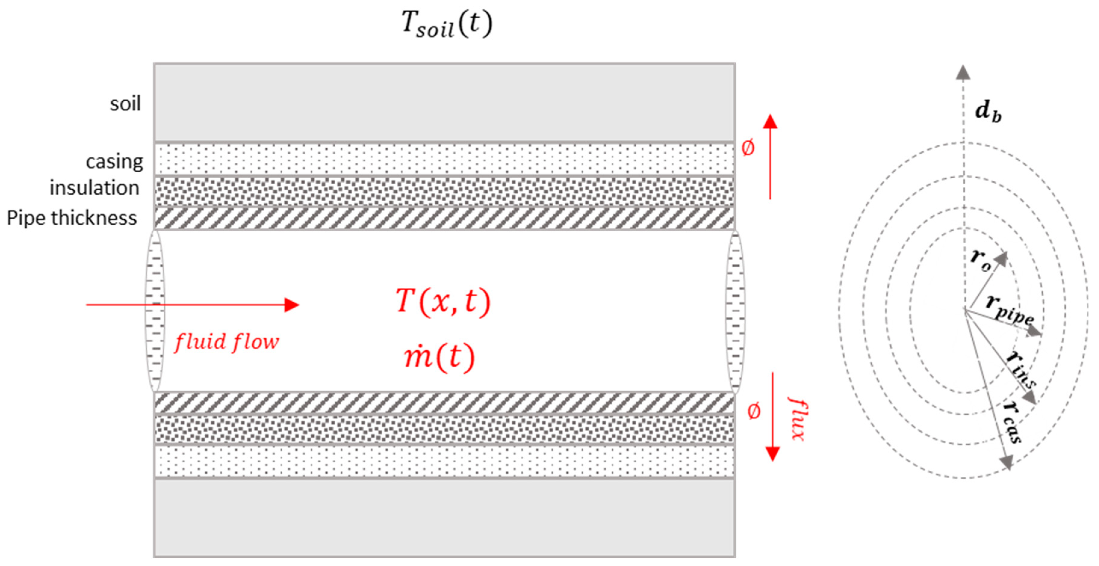
2.2. Physical Modelling of the Distribution Section

The distribution section consists of $nb$ branches, and each branch $b$ has a number of consumer components, $n{c}_b$. This paper models a consumer component $c$ in a branch $b$ for easy generalisation. As described, a consumer component $c$ has a main pipe $mp$, an extended-in pipe $e{p}_{in}$, an extended-out pipe $e{p}_{out}$, a return pipe $rp$, a splitter, and a mixer, which are connected as shown in Figure 3.

Distribution splitter model:

$$\mathrm{Mass} \mathrm{balance} {\dot{m}}_{b,c,mp}\left(\mathrm{t}\right)={\dot{m}}_{b,c+1,mp}\left(t\right)+{\dot{m}}_{b,c,e{p}_{in}}\left(t\right)$$

(6)

$$\mathrm{Temperature} \mathrm{equality} T_{b,c,mp,f}\left(t\right)=T_{b,c+1,mp,0}\left(t\right)=T_{b,c,e{p}_{in},0}\left(t\right)$$

(7)

Distribution mixer model:

$$\mathrm{Mass} \mathrm{balance} {\dot{m}}_{b,c,rp}\left(t\right)={\dot{m}}_{b,c,e{p}_{out}}\left(t\right)+{\dot{m}}_{b,c+1,rp}\left(t\right)$$

(8)

$$\mathrm{Energy} \mathrm{balance} T_{b,c,rp,0}\left(t\right)={\displaystyle \frac{{\dot{m}}_{b,c,e{p}_{out}}\left(t\right)T_{b,c,e{p}_{out},f}\left(t\right)+{\dot{m}}_{b,c+1,rp}\left(t\right)T_{b,c+1,rp,f}\left(t\right)}{{\dot{m}}_{b,c,rp}\left(t\right)}}$$

(9)

Substation (heat exchanger) model:

$$\mathrm{Mass} \mathrm{balance} {\dot{m}}_{b,c,e{p}_{out}}\left(t\right)={\dot{m}}_{b,c,e{p}_{in}}\left(\mathrm{t}\right)$$

(10)

$$\mathrm{Energy} \mathrm{balance} P_{demand,c }\left(t\right)={\dot{m}}_{b,c,e{p}_{in}}\left(t\right)C_p\left(T_{b,c,e{p}_{in},f}\left(t\right)-T_{b,c,e{p}_{out},0}\left(t\right)\right)$$

(11)

It can be observed that the pipes in both the distribution and generation sections have not been modelled. However, their modelling approach remains the same, irrespective of their location in the network configuration. A pipe $pk$, as shown in Figure 4, is modelled based on the assumptions stated in [14,25,26], which are outlined below:

⮚

Heat transfer occurs solely in the radial direction.

⮚

Conduction heat transfer is considered through the pipe, insulation, casing, and soil.

⮚

Material properties are constant and independent of temperature.

⮚

Thermal interactions between the supply and return pipes are not accounted for.

⮚

The thermal inertia of the pipes, casing, and insulation is neglected.

⮚

Bent pipes are treated as straight pipes of the same length.

where $\forall pk=pmp,prp,e{p}_{in},e{p}_{out},mp,rp$.

$${\displaystyle \frac{\partial T\left(x,t\right)}{\partial t}}+{\displaystyle \frac{\dot{m}\left(t\right)}{\rho A}}{\displaystyle \frac{\partial T\left(x,t\right)}{\partial x}}=B\left(t\right)\left(T_{soil}\left(t\right)-T\left(x,t\right)\right) B\left(t\right)={\displaystyle \frac{\pi D_{i}U\left(t\right)}{\rho c_{p}A}}$$

(12)

The pipe model given in $\left(12\right)$ is a two-dimensional (2D) partial differential equation (PDE) in space and time, which is best solved by discretising one or both independent domains. In this research, the spatial temperature derivatives are approximated using second-order finite differences to balance model complexity and computation time. Specifically, the second-order central difference method is applied to approximate all the spatial temperature derivatives except the last point, as shown in $\left(13\right)$ and $\left(14\right)$, while the second-order backward difference method is used for the last spatial temperature derivative, as shown in $\left(14\right)$. This spatial discretisation transforms the physical model from a PDE into a set of ordinary differential equations (ODEs).

$$\begin{gathered} T_1\left(t\right)=T_{inlet}\left(t\right) \\ {\displaystyle \frac{d{T}_i\left(t\right)}{dt}}=-\left({\displaystyle \frac{\dot{m}\left(t\right)}{2\rho A\Delta x}}\right)(T_{i+1}\left(t\right)-T_{i-1}\left(t\right))+B\left(t\right)(T_{soil}\left(t\right)-T_i\left(t\right)) \forall i=2\cdots n-1 \end{gathered}$$

(13)

$${\displaystyle \frac{d{T}_n\left(t\right)}{dt}}=-\left({\displaystyle \frac{\dot{m}\left(t\right)}{2\rho A\Delta x}}\right)(T_{n-2}\left(t\right)-4T_{n-1}\left(t\right)+3T_n\left(t\right))+B\left(t\right)(T_{soil}\left(t\right)-T_n\left(t\right))$$

(14)

Having developed the physical model of a DHN, the grey-box linear parameter varying (LPV) modelling of the network generation and distribution sections will be introduced.

2.3. Grey-Box Modelling of the Generation and Distribution Section

The model equations for the mixers, splitters, and substations (heat exchangers) in the generation and distribution sections are purely algebraic and, therefore, remain unchanged during the grey-box modelling. However, the primary computation challenge in the DHN physical modelling lies in the pipe models. Thus, a grey-box model is developed specifically for the pipes in the network. Since the modelling approach for all pipes is the same, a grey-box LPV model is formulated for a single pipe $pk$.

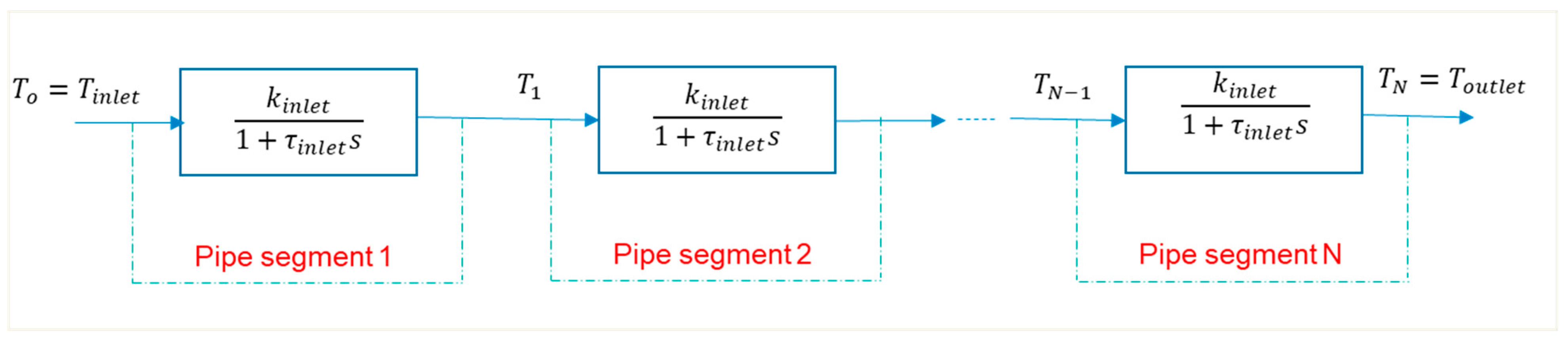
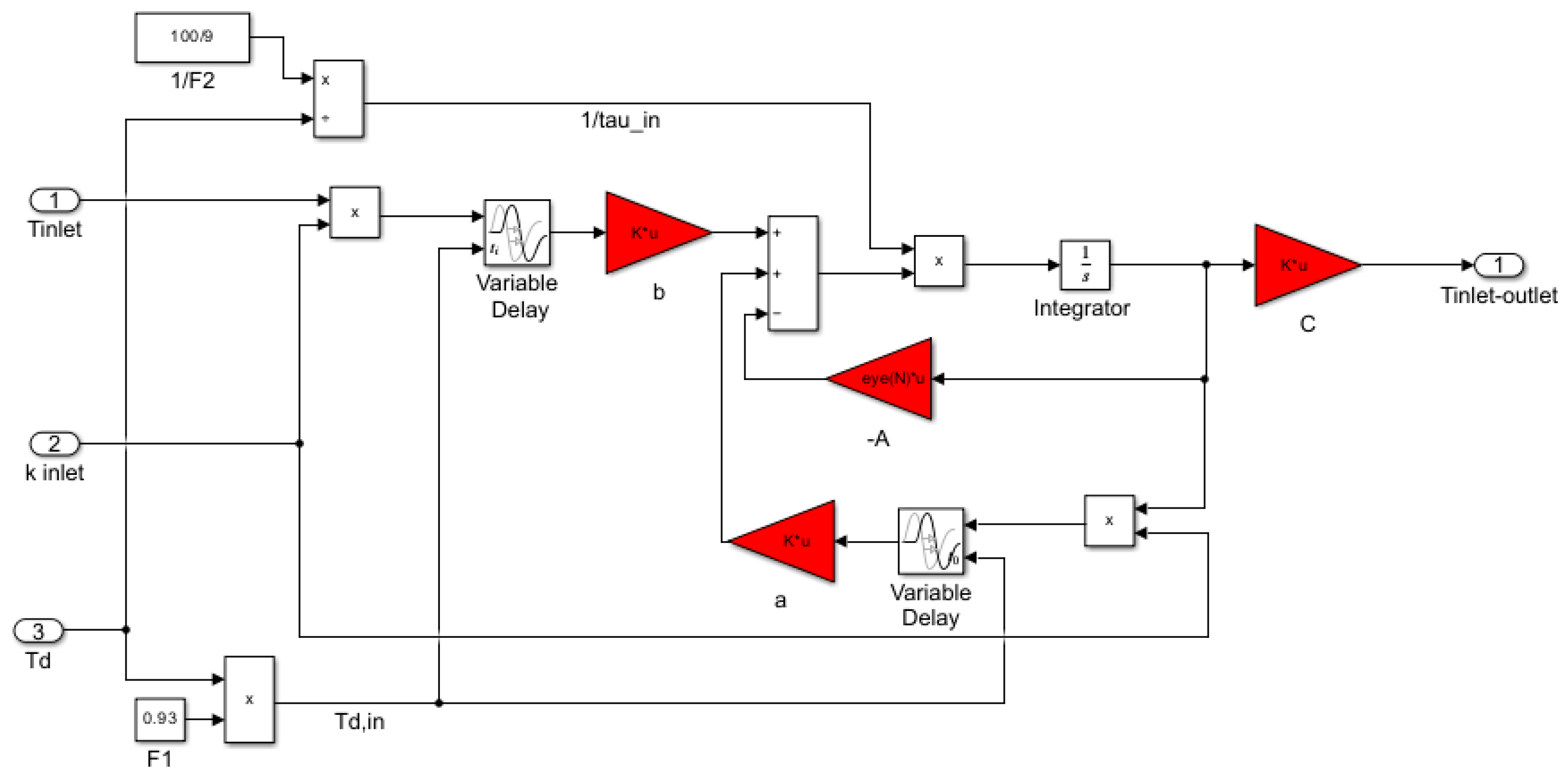
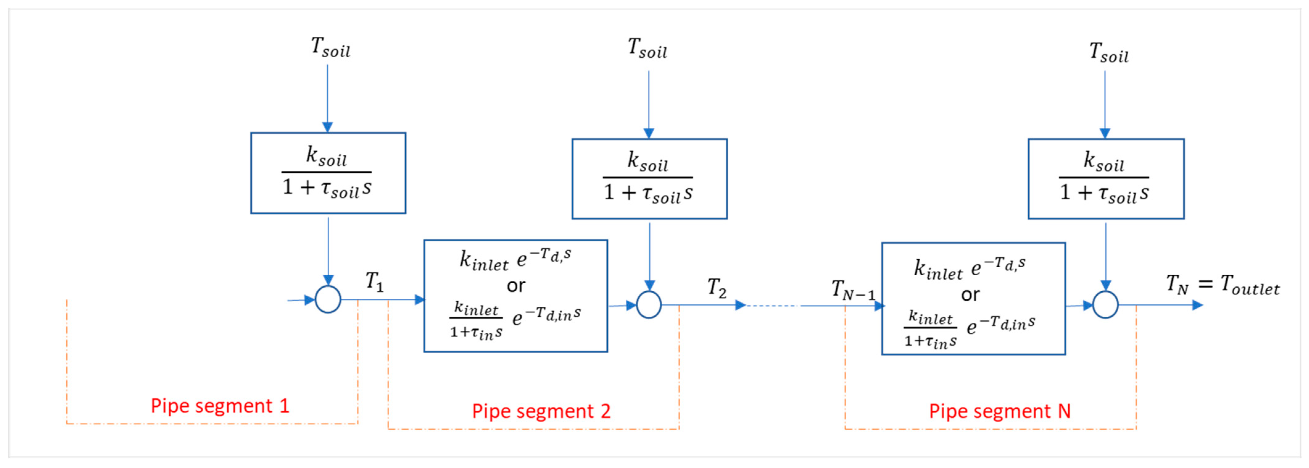
2.3.1. LPV Modelling of a Pipe

An LPV model is a linear model whose parameters depend on scheduling variables, which may vary over time. The principal objective of the LPV modelling technique is to explicitly capture the system dynamics while maintaining computational efficiency. The general formulation of a single input ($u$), single output ($y$) (SISO) linear model can be mathematically shown in the time domain in $\left(15\right)$.

$$a_{\alpha }{\displaystyle \frac{d^{\alpha }y\left(t\right)}{d{t}^{\alpha }}}+a_{\alpha -1}{\displaystyle \frac{d^{\alpha -1}y\left(t\right)}{d{t}^{\alpha -1}}}+\cdots +a_1{\displaystyle \frac{dy\left(t\right)}{dt}}+a_{0}y\left(t\right)=b_{\beta }{\displaystyle \frac{d^{\beta }u\left(t-T_d\right)}{d{t}^{\beta }}}+b_{\beta -1}{\displaystyle \frac{d^{\beta -1}u\left(t-T_d\right)}{d{t}^{\beta -1}}}+\cdots +b_1{\displaystyle \frac{du\left(t-T_d\right)}{dt}}+b_{0}u\left(t-T_d\right)$$

(15)

where $a=\left[a_{\alpha },a_{\alpha -1}\cdots a_0\right]$, $b=[b_{\beta },b_{\beta -1}, \cdots , b_{\beta }]$, and delay $T_d$ are the model parameters dependent on the scheduling variables of an LPV model. This high-order linear model can be transformed into a state-space representation or expressed in the Laplace domain, as shown in $\left(16\right)$, to facilitate its resolution.

$${\displaystyle \frac{y\left(s\right)}{u\left(s\right)}}={\displaystyle \frac{b_{\beta }{s}^{\beta }+b_{\beta -1}{s}^{\beta -1}+\cdots +b_{1}s+b_0}{a_{\alpha }{s}^{\alpha }+a_{\alpha -1}{s}^{\alpha -1}+\cdots +a_{1}s+a_0}}{e}^{-\tau s}=G\left(s\right)e^{-T_{d}s}$$

(16)

where $\alpha$ and $\beta$ are the number of poles and zeros, respectively.

The principal assumption of this LPV model is that the model parameters $a$, $b$, and $T_d$ must be constant with time. If this assumption is violated, a slight modification must be introduced to the LPV model to ensure its feasibility and predictive capability for continuous dynamic systems. LPV models incorporating such modifications are referred to as modified or quasi-LPV models. The steps for formulating this LPV model are now outlined.

2.3.2. Steps for Formulating LPV Models

The following are the steps for formulating an LPV model:

• Step 1: Scheduling parameter or variable identification

The scheduling parameters, also known as the scheduling variables, are part of the input variables of a nonlinear physical model. When these variables remain constant, the nonlinear model becomes linear. During the development of an LPV model, these scheduling variables are no longer part of the input variables.

• Step 2: Linear model development

Develop a linear model that shows the relationship between an output variable and the input variables at given values of the scheduling variables. This linear model development can be achieved through global and local approaches [19]. In the global approach, the dataset for the model development is obtained by exciting all the input variables simultaneously, so a Multiple Input Single Output (MISO) development is identified. In the local approach, Single Input Single Output (SISO) models are independently built and combined to form a MISO model by leveraging the superposition advantage of linear models.

• Step 3: Generating data and identifying the relationship between model parameters and the scheduling variables

Generate a dataset that records the linear model parameters at given values of the scheduling variables. Then, machine learning, curve fitting, or system identification techniques are employed to find the relationship between the model parameters and the scheduling variables.

• Step 4: Finalise the LPV model

Express the output variable as a function of the input variables and model parameters. Then, establish the relationship between the model parameters and the scheduling variables.

The outlined steps for formulating an LPV model are followed in this paper to develop the LPV model of a pipe.

• Step 1: Scheduling variable identification

Examining the nonlinear physical pipe model in $\left(13\right)$ and $\left(14\right)$, it can be observed that the input variables are the pipe inlet temperature $T_{inlet}\left(t\right)$, soil temperature $T_{soil}\left(t\right)$, and mass flow rate $\dot{m}\left(t\right)$, and the output variable is the pipe outlet temperature $T_n\left(t\right)=T_{outlet}\left(t\right)$. If the mass flow rate remains constant over time, the nonlinear model becomes linear. Therefore, the mass flow rate is the scheduling variable and is excluded from the set of input variables. Consequently, the input variables to be considered during the LPV model development of a pipe are the pipe inlet temperature and soil temperature.

• Step 2: Linear Model Development

Here, a linear model that shows the relationship between the output variable (pipe outlet temperature) and the input variables (pipe inlet temperature and soil temperature) is developed. The local approach was considered for the LPV modelling of a heat exchanger in [20] because the simultaneous long-range excitation of all the input variables of the heat exchanger is not possible in practice. Similarly, in a real-life district heating system, the simultaneous long-range excitation of all the input variables of a pipe is not feasible, so the local approach is also adopted for the linear model development in this paper.

As discussed earlier, the local approach involves developing an independent SISO model for the relationship between the output variable and each input variable. Therefore, two SISO models are developed: one showing the relationship between pipe outlet temperature $T_{outlet}\left(t\right)$ and pipe inlet temperature $T_{inlet}\left(t\right)$, represented by $T_{outlet}\left(t\right)=f\left(T_{inlet}\left(t\right),{\theta }_{inlet}\right)$, and the other showing the relationship between the pipe outlet temperature $T_{outlet}\left(t\right)$ and soil temperature $T_{soil}\left(t\right)$, represented by $T_{outlet}\left(t\right)=f\left(T_{soil}\left(t\right),{\theta }_{soil}\right)$. Finally, these two SISO models are combined to obtain a MISO model that shows the relationships between the pipe outlet temperature, inlet temperature, and soil temperature, as given in $\left(17\right)$:

$$T_{outlet}\left(t\right)=f\left(T_{inlet}\left(t\right), T_{soil}\left(t\right),\theta \right)$$

(17)

where ${\theta }_{inlet}$ and ${\theta }_{soil}$ are sets of model parameters that depend on the scheduling variable (mass flow rate), and $\theta$ is a set of ${\theta }_{inlet}$ and ${\theta }_{soil}$.

Let us now develop the SISO models, starting with $T_{outlet}\left(t\right)=f\left(T_{inlet}\left(t\right),{\theta }_{inlet}\right)$.

The SISO linear model that shows the relationship between $T_{outlet}\left(t\right)$ and $T_{inlet}\left(t\right)$.

The general SISO linear model given in $\left(15\right)$ is employed to develop the linear relationship between $T_{outlet}\left(t\right)$ and pipe inlet temperature $T_{inlet}\left(t\right)$.

Relative to the physical model, pipe discretisation can also be performed during the LPV model development to find the best SISO linear model for each discretised pipe segment. Thus, the linear model for each discretised pipe model can be combined to produce a single-pipe model. In addition, the physics of fluid flow in a pipe states that a fluid element into a pipe segment will take some time before it arrives at the pipe segment outlet. This time of travel is known as the delay. This implies that a time delay not equal to zero ($T_d\ne 0)$ is possible in $\left(15\right)$. Therefore, linear models with $T_d\ne 0$ and $T_d=0$ are tested. To minimise model complexity, the number of zeros is assumed to be zero $\left(\beta =0\right)$, and the number of poles (also known as the order of the linear model) is assumed to be less than two ($\alpha <2)$. Consequently, three case study models are possible to develop the relationship between $T_{outlet}\left(t\right)$ and $T_{inlet}\left(t\right)$. These models are shown in the Laplace domain in Figure 5, Figure 6, and Figure 7, respectively. The first-order model without delay in Figure 5 is regarded as the linearised model (model A) in this research, the zero-order model with delay in Figure 6 is regarded as the globalised linear model (model B), and the first-order model with delay in Figure 7 is called the distributed linear model (model C).

It should be noted that the numbers of discretised pipe segments in the physical and grey-box models are not equal: $n \ne N$.

At this stage, it is possible to identify the model parameters $k_{inlet}$, ${\tau }_{inlet}$, $T_d$, ${\tau }_{in}$, and $T_{d,in}$ since the model structures have been formulated. These model parameters are members of the set ${\theta }_{inlet}$. According to the LPV modelling steps, these model parameters should be obtained at given values of the scheduling variables (mass flow rate) bounded by ${\dot{m}}_{min}<\dot{m}<{\dot{m}}_{max}$ by the exciting input variable ($T_{inlet}$) for all the three possible model structures. However, this could be somewhat cumbersome. As a result, this research decided to obtain the values of some model parameters from the physical model analytically. Firstly, the spatial temperature derivative in the physical pipe model in $\left(12\right)$ is approximated with the first-order backward difference formula, as shown in $\left(18\right)$, with the purpose of developing a reduced order model. Laplace transformation is then imposed on the physical model at constant soil temperature to yield $\left(19\right)$. Finally, $\left(19\right)$ is rearranged to yield $\left(20\right)$, which is then compared with model A (first-order LPV model without delay) in Figure 5 to identify some model parameters ($k_{inlet}$ and ${\tau }_{inlet}$). The time delay $T_d$ can be computed using the mass continuity equation. Therefore, three out of the five model parameters ($k_{inlet}$, ${\tau }_{inlet}$, $T_d$) have been successfully identified, as shown in $\left(21\right)$, $\left(22\right)$, and $\left(23\right)$.

$${\displaystyle \frac{d{T}_{\left.i(t\right)}}{dt}}=-\left({\displaystyle \frac{\dot{m}\left(t\right)}{\rho A\Delta x}}+B\left(t\right)\right)T_i\left(t\right)+B\left(t\right)T_{soil}\left(t\right)+{\displaystyle \frac{\dot{m}\left(t\right)}{\rho A\Delta x}}{T}_{i-1}\left(t\right)$$

(18)

$$s{T}_i\left(\mathrm{s}\right)-T_i\left(0\right)=-\left({\displaystyle \frac{\dot{m}}{\rho A\Delta x}}+B\right)T_i\left(s\right)+{\displaystyle \frac{\dot{m}}{\rho A\Delta x}}{T}_{i-1}\left(\mathrm{s}\right)$$

(19)

$$T_i\left(\mathrm{s}\right)={\displaystyle \frac{\frac{\dot{m}}{\rho A\Delta x}/(\frac{\dot{m}}{\rho A\Delta x}+B)}{\frac{1}{\left(\frac{\dot{m}}{\rho A\Delta x}+B\right)}s+1}}{T}_{i-1}\left(\mathrm{s}\right)$$

(20)

Therefore, the model parameters are

$$k_{inlet}={\displaystyle \frac{\frac{\dot{m}}{\rho A\Delta x}}{\frac{\dot{m}}{\rho A\Delta x}+B}}$$

(21)

$$T_d={\displaystyle \frac{\rho A\Delta x}{\dot{m}\left(t\right)}}$$

(22)

$${\tau }_{inlet}={\displaystyle \frac{1}{\frac{\dot{m}}{\rho A\Delta x}+B}}$$

(23)

$$N={\displaystyle \frac{L}{\Delta x}}$$

(24)

This model identification technique implies that model A is similar to the first-order physical pipe model, which implicitly accounts for the delay. While model B is a delayed model without any time-constant dynamics, model C incorporates time-constant (${\tau }_{in}$) dynamics and explicitly accounts for the delay with $T_{d,in}$. So, $T_{d,in}<$ $T_d$, because $T_d$ represents the complete delay in a pipe segment, part of which has already been provided by ${\tau }_{in}$. Therefore, $T_{d,in}$ and ${\tau }_{in}$ can be computed using $T_{d,in}=F_1{T}_d$ and ${\tau }_{in}=F_2{T}_d$, where $F_1$ and $F_2$ are constants to be determined. Thus, the identification of the $T_{d,in}$ and ${\tau }_{in}$ for model C depends on the values of $F_1$ and $F_2$.

$F_1$ and $F_2$ are determined using system identification techniques. First, a dataset is generated by simulating the nonlinear physical pipe model with given profiles of the input and scheduling variables. A pseudo-step change, given in $\left(30\right)$, is applied to the pipe inlet temperature $T_{inlet}$ at a specified step-change time, while a step change in mass flow rate is imposed at a later time, and a constant soil temperature is considered. The pipe outlet temperature profile obtained from the simulation of the physical model is regarded as the actual pipe outlet temperature. Model C is then implemented in Simulink with initial guess values for $F_1$ and $F_2$. A grid search optimisation algorithm is used to obtain the optimal values of $F_1$ and $F_2$ that best minimise the objective function. The objective function is defined as the sum of the relative errors between the actual pipe outlet temperature and predicted pipe outlet temperature from the Simulink model. The optimal values of $F_1$ and $F_2$ obtained from the optimisation process are then used to identify $T_{d,in}$ and ${\tau }_{in}$. As a result, the set of model parameters ${\theta }_{inlet}$, which defines the relationship between the pipe outlet temperature $T_{outlet}\left(t\right)$ and pipe inlet temperature $T_{inlet}\left(t\right)$, has been successfully identified.

Figure 5, Figure 6 and Figure 7 can be then transformed into mathematical formulas to derive the relationship between the outlet temperature and the inlet temperature for models A, B, and C, as shown in $\left(25\right)$, $\left(26\right)$, and $\left(27\right)$, respectively.

$$T_{outlet}^{inlet}\left(s\right)={\left[{\displaystyle \frac{k_{inlet}}{{\tau }_{inlet}s+1}}\right]}^N{T}_{inlet}\left(s\right)$$

(25)

$$T_{outlet}^{inlet}\left(s\right)={\left[k_{inlet}{e}^{-T_d}\right]}^N{T}_{inlet}\left(s\right)$$

(26)

$$T_{outlet}^{inlet}\left(s\right)={\left[{\displaystyle \frac{k_{inlet}}{{\tau }_{in}s+1}}{e}^{-T_{d,in}}\right]}^N{T}_{inlet}\left(s\right)$$

(27)

where $T_{outlet}^{inlet}$ denotes the influence of the inlet temperature on the pipe outlet temperature.

Having completed the model structure development and parameter identification, the best model structure among models A, B, and C can be selected through model evaluation using the coefficient of determination ($R^2$) and percentage fit formulas given in $\left(28\right)$ and $\left(29\right)$, respectively, as the evaluation metrics. The simulation result of each grey-box model (A, B, and C) is validated against that of the physical model of a single pipe. Consider a first case study where a non-adiabatic pipe of 0.31 m diameter, 200 m length, having thermophysical properties listed in Appendix A.2, transmits hot water at the inlet temperature described in $\left(30\right)$. The inlet temperature undergoes a pseudo-step change at 60 s from 90 °C to 95 °C. The pipe operates with a constant mass flow rate 80 $\mathrm{kg}/\mathrm{s}$ and is influenced by a constant soil temperature of 0 °C. A 0.5 m length pipe segment is used for the physical model spatial discretisation, ensuring that the delay from the simulation result matches the physical delay calculated using the mass continuity equation. The simulation runs for 2400 s, and the physical model is simulated in MATLAB with ode15s, a variable step–variable order (VSVO) solver employing the numerical differentiation formula (NDF). The absolute and relative tolerances are set to 1 × 10⁻¹⁰ and 1 × 10⁻⁹, respectively. The N values of the grey-box models, sufficient to capture the pipe dynamics without numerical problems, are 100, 180 (calculated using a Courant number of 1 for explicit models), and 28 for models A, B, and C, respectively. In this example, the general hypothesis of an LPV model is not violated because the scheduling variable (mass flow rate) is constant with time. Therefore, models A, B, and C are used as linear parameter-varying models without any modification. These models can be directly simulated in MATLAB using the ‘lsim’ function by declaring them as transfer function models. After model resolution, the pipe outlet temperatures obtained from simulating the physical model and the three-case study LPV models are illustrated in Figure 8.

$${R^2}_{pk}=1-{\displaystyle \frac{{{\displaystyle \sum }}_{ti}^{nti}{\left(T_{pk}\left(t_{ti}\right)-\widehat{T_{pk}}(t_{ti})\right)}^2}{{{\displaystyle \sum }}_{ti}^{nti}{\left(T_{pk}\left(t_{ti}\right)-\overline{T_{pk}}\right)}^2}}$$

(28)

$$\% fi{t}_{pk}=1-\sqrt{{\displaystyle \frac{{{\displaystyle \sum }}_{ti}^{nti}{\left(T_{pk}\left(t_{ti}\right)-\widehat{T_{pk}}(t_{ti})\right)}^2}{{{\displaystyle \sum }}_{ti}^{nti}{\left(T_{pk}\left(t_{ti}\right)-\overline{T_{pk}}\right)}^2}}}$$

(29)

$$T_{inlet}\left(t\right)=T_{inlet\_start}+{\displaystyle \frac{T_{inlet\_step}}{1+exp\left(-\frac{(t-t_{step\_change}}{3.6}\right)}}$$

(30)

where $T_{inlet\_start}$ is the initial value of the inlet temperature, $T_{inlet\_step}$ is the step change of the inlet temperature, and $t_{step\_change}$ is the time at which the step change is imposed on the inlet temperature.

It is important to note that the percentage fits and $R^2$ values are calculated over the region where significant changes occur in the input variables and where these changes have a measurable impact on the output variable. Therefore, it can be observed that models A, B, and C fit 84.4%, 99.51%, and 90.63% of the physical model results, respectively, with $R^2$ values of 0.976, 1, and 0.991. Since the percentage fit and $R^2$ of model A are considerably lower than those of models B and C, it can be eliminated from consideration. The best model between models B and C can be selected by exciting the mass flow rate from 40 $\mathrm{kg}/\mathrm{s}$ abruptly to 80 $\mathrm{kg}/\mathrm{s}$ at 1200 s, along with the pseudo-step changed inlet temperature in the first case study at a constant soil temperature of 0 °C. In this case study, the LPV modelling assumption has been violated because the variation in the scheduling variable (mass flow rate) causes the model parameters to change with time. Therefore, models B and C are employed as modified LPV models. The thermal conductivities of the insulation and casing in Appendix A.2 were changed to that of the pipe material to increase the heat losses and assess the model’s efficiency under stringent conditions. Since varying the model parameters of a Laplace model is more effortless in Simulink, the simulation was transferred to Simulink. Thus, the Simulink representation of model B can be found in Figure 9. In addition, to allow the possibility of changing the number of discretisation N for any pipe length, model C is converted to a delayed-state space model ($\left(31\right)$ to $\left(36\right)$), with the Simulink representation in Figure 10.

$${\tau }_{in}\dot{T_{gb}}\left(t\right)=A{T}_{gb}\left(t\right)+B{T}_{inlet}\left(t\right)+a{T}_{gb}\left(t-T_{d,in}\right)+b{T}_{inlet}\left(t-T_{d,in}\right)$$

(31)

$$T_{outlet}^{inlet}\left(t\right)=C{T}_{gb}\left(t\right)$$

(32)

where $T_{gb}\in R^{N\times 1}$ is a vector of the discretised temperature that shows the influence of the inlet temperature on the pipe outlet temperature; $A, a,B,b,C$ are the modified LPV model parameters, $B=0, B\in R^{N\times 1}$.

$$A=-I, A\in R^{N\times N}$$

(33)

$$a=k_{inlet}\left[\begin{array}{c}\begin{array}{ccc}\begin{array}{ccc}0& 0& 0\end{array}& \begin{array}{ccc}.& .& .\end{array}& 0\end{array}\\ \begin{array}{ccc}\begin{array}{ccc}1& 0& 0\end{array}& \begin{array}{ccc}.& .& .\end{array}& 0\end{array}\\ \begin{array}{ccc}\begin{array}{ccc}0& 1& 0\end{array}& \begin{array}{ccc}.& .& .\end{array}& 0\end{array}\\ \begin{array}{ccc}\begin{array}{ccc}.& .& .\end{array}& \begin{array}{ccc}.& .& .\end{array}& 0\end{array}\\ \begin{array}{ccc}\begin{array}{ccc}0& 0& .\end{array}& \begin{array}{ccc}.& .& 1\end{array}& 0\end{array}\end{array}\right], a\in R^{N\times N}$$

(34)

$$b=\left[\begin{array}{c}1\\ 0\\ .\\ .\\ .\\ 0\end{array}\right], b\in R^{N\times 1}$$

(35)

$$C=\left[\begin{array}{ccc}0& .& .\end{array}\begin{array}{ccc}.& 0& 1\end{array}\right], C\in R^{1\times N}$$

(36)

The pipe outlet temperature for this second case study is illustrated in Figure 11 for models B and C. The $R^2$ values and percentage fit of models B and C at the region of mass flow rate variation only are (−1.053, −43.27%) and (0.996, 93.63%), respectively. This implies that model B could not capture the dynamics induced by the mass flow rate variation. Therefore, model C is the best LPV model, as it effectively demonstrates the relationship between the pipe inlet and outlet temperatures. This research proceeds to develop the LPV model that shows the relationship between the pipe outlet temperature and the soil temperature. The transfer function model in $\left(27\right)$ and the state space models in $(\left(31\right)$ to $\left(36\right)$) represent the relationship between the inlet temperature and the pipe outlet temperature.

The SISO linear model that shows the relationship between $T_{outlet}\left(t\right)$ and $T_{soil}\left(t\right)$.

Relying on the physical knowledge of a pipe operation, the soil temperature influence on the pipe is distributed over the pipe length. Therefore, the LPV model structure is formulated as a distributed delay model, as shown in Figure 12.

Figure 12 shows that this SISO (soil temperature influence) model depends on both the inlet and soil temperature influences. Therefore, these influences are captured separately.

Although model C has been identified as the best LPV model for describing the relationship between pipe outlet and inlet temperature, it is also important to assess the feasibility of using model B to capture the dynamics of the inlet temperature influence in this SISO model. The reason is that model B is less complex than model C, and it could leverage the distribution delay effect to account for the dynamics of the inlet temperature influence. Consequently, two mathematical models are developed for the SISO model that demonstrate the relationship between the pipe outlet and soil temperature. Thus, these models are referred to as soil influence model B $\left(37\right)$ and soil influence model C $\left(39\right)$.

For soil influence model B, Figure 12 can be translated to a mathematical equation in $\left(37\right)$:

$${\displaystyle \frac{T_{outlet}^{soil}\left(\mathrm{s}\right)}{T_{soil}\left(s\right)}}={\displaystyle \frac{k_{soil}}{1+{\tau }_{soil}s}}{\displaystyle \sum }_{i=0}^{N-1}{k_{inlet}}^i{e}^{-i{T}_{d}s}$$

(37)

${\displaystyle \sum }_{i=0}^{N-1}{\left(k_{inlet}\right)}^i{e}^{-i{T}_{d}s}$ corresponds to the sum of a geometric series with a common ratio of $k_{inlet}{e}^{-T_{d}s}$, and first term equals 1. This term can be replaced with the general formula for summing a geometric series to give $\left(38\right)$:

$${\displaystyle \frac{T_{outlet}^{soil}\left(\mathrm{s}\right)}{T_{soil}\left(s\right)}}={\displaystyle \frac{k_{soil}}{1+{\tau }_{soil}s}}{\displaystyle \frac{1-{\left(k_{inlet}\right)}^N{e}^{-N{T}_{d}s}}{1-k_{inlet}{e}^{-T_{d}s}}}$$

(38)

Also, the soil influence model C can be formulated from Figure 12, as expressed in $\left(39\right)$,

$${\displaystyle \frac{T_{outlet}^{soil}\left(\mathrm{s}\right)}{T_{soil}\left(s\right)}}={\displaystyle \frac{k_{soil}}{1+{\tau }_{soil}s}}{\displaystyle \sum }_{i=0}^{N-1}{\left({\displaystyle \frac{k_{inlet}}{1+{\tau }_{in}s}}\right)}^i{e}^{-i{T}_{d,in}s}$$

(39)

and its transformation yields $\left(40\right)$:

$${\displaystyle \frac{T_{outlet}^{soil}\left(\mathrm{s}\right)}{T_{soil}\left(s\right)}}={\displaystyle \frac{k_{soil}}{1+{\tau }_{soil}s}}{\displaystyle \frac{1-{\left(\frac{k_{inlet}}{1+{\tau }_{in}s}\right)}^N{e}^{-N{T}_{d,in}s}}{1-\frac{k_{inlet}}{1+{\tau }_{in}s}{e}^{-T_{d,in}s}}}$$

(40)

Having developed the model structures, it is imperative to find the relationship between model parameters $k_{soil}$ and ${\tau }_{soil}$ and the scheduling parameter (mass flow rate). This relationship can be obtained by applying Laplace transformation to $\left(18\right)$ at a constant pipe inlet temperature to yield $\left(41\right)$:

$$s{T}_i\left(\mathrm{s}\right)-T_i\left(0\right)=-\left({\displaystyle \frac{\dot{m}}{\rho A\Delta x}}+B\right)T_i\left(s\right)+B{T}_{soil}\left(\mathrm{s}\right)$$

(41)

$$T_i\left(\mathrm{s}\right)={\displaystyle \frac{B/(\frac{\dot{m}}{\rho A\Delta x}+B)}{\frac{1}{\left(\frac{\dot{m}}{\rho A\Delta x}+B\right)}s+1}}{T}_{soil}\left(\mathrm{s}\right)$$

(42)

Therefore, $k_{soil}={\displaystyle \frac{B}{\frac{\dot{m}}{\rho A\Delta x}+B}}$ and ${\tau }_{soil}=1/\left({\displaystyle \frac{\dot{m}}{\rho A\Delta x}}+B\right)$.

• Step 3: Generating the dataset and identifying the relationship between model parameters and scheduling variables

During the development of the SISO linear models, two classes of model parameters were identified:

• Parameters that vary with the scheduling variables (mass flow rate), which include $k_{inlet}$, $k_{soil}$, ${\tau }_{inlet}$, ${\tau }_{soil}$, $T_d$, ${\tau }_{in}$, and $T_{d,in}$.
• Parameters that remain constant with the scheduling variable, which are $F_1$ and $F_2$.

Since the relationships between the model parameters and the mass flow rate have been directly identified from the physical knowledge of the system, implementing this step is unnecessary.

• Step 4: LPV Model Finalisation

Here, the developed LPV SISO models can be combined into a single LPV MISO model using the superposition principle:

$$T_{outlet}\left(s\right)=T_{outlet}^{inlet}\left(\mathrm{s}\right)+T_{outlet}^{soil}\left(\mathrm{s}\right)$$

(43)

As the optimal soil influence model is yet to be determined, two pipe models are compared: model CC $\left(44\right)$, which uses model C for both inlet and soil temperature influences, and model CB $\left(45\right)$, which uses model C for the inlet temperature influence and model B for the soil temperature influence.

$$T_{outlet}\left(\mathrm{s}\right)={\left[{\displaystyle \frac{k_{inlet}\left(\dot{m}\right)}{1+{\tau }_{in}\left(\dot{m}\right)s}}{e}^{-T_{d,in}\left(\dot{m}\right)s}\right]}^N{T}_{inlet}\left(s\right)+{\displaystyle \frac{k_{soil}\left(\dot{m}\right)}{1+{\tau }_{soil}\left(\dot{m}\right)s}}{\displaystyle \frac{1-{\left(\frac{k_{inlet}\left(\dot{m}\right)}{1+{\tau }_{in}\left(\dot{m}\right)s}\right)}^N{e}^{-N{T}_{d,in}\left(\dot{m}\right)s}}{1-\frac{k_{inlet}\left(\dot{m}\right)}{1+{\tau }_{in}\left(\dot{m}\right)s}{e}^{-T_{d,in}\left(\dot{m}\right)s}}}{T}_{soil}\left(s\right)$$

(44)

$$T_{outlet}\left(\mathrm{s}\right)={\left[{\displaystyle \frac{k_{inlet}\left(\dot{m}\right)}{1+{\tau }_{in}\left(\dot{m}\right)s}}{e}^{-T_{d,in}\left(\dot{m}\right)s}\right]}^N{T}_{inlet}\left(s\right)+{\displaystyle \frac{k_{soil}\left(\dot{m}\right)}{1+{\tau }_{soil}\left(\dot{m}\right)s}}{\displaystyle \frac{1-{\left(k_{inlet}\left(\dot{m}\right)\right)}^N{e}^{-N{T}_d\left(\dot{m}\right)s}}{1-k_{inlet}\left(\dot{m}\right)e^{-T_d\left(\dot{m}\right)s}}}{T}_{soil}\left(s\right)$$

(45)

A third case study is conducted to determine the optimal single-pipe model between models CB and CC. The pipe inlet temperature undergoes a pseudo-step change from 90 °C to 95 °C at 60 s using the sigmoid function in $\left(30\right)$, and the soil temperature and mass flow rate undergo a step change from –5 °C to 35 °C at 600 s and 40 $\mathrm{kg}/\mathrm{s}$ to 90 $\mathrm{kg}/\mathrm{s}$ at 1200 s, respectively. Also, the thermal conductivity of the pipe material is assumed to be the same as that of the insulation and casing. The simulation spans from 0 to 2400 s, using $N=28$ for the grey-box models and $\Delta x=0.5$ m for the physical model. The grey-box model is solved using a fixed-step ode3 solver, based on the Bogacki–Shampine algorithm, using a fixed time step of 1 s. The computation times for the physical model and models CB and CC are 1.86 s, 0.38 s, and 0.39 s, respectively, conducted on a Windows 10 DELL PC with 32 GB RAM, a 12th Gen Intel(R) Core (TM) i7-12700H processor, and a clock speed of 2.30 GHz. After simulation, the pipe outlet temperatures obtained from the physical model and models CB and CC are shown in Figure 13, with both BC and CC achieving an overall average $R^2$ value of 0.993 and a percentage fit of 91.5% against the physical model.

Since models CB and CC have similar computation times and percentage fits against the physical model, either can serve as the grey-box single-pipe model. However, the less complex model, in terms of the model order, is recommended for optimisation tasks. Thus, model CB is the preferred grey-box pipe model for predicting or estimating a pipe outlet temperature as a function of the inlet temperature, soil temperature, mass flow rates, and thermophysical properties. A large step change was imposed on the soil temperature and mass flow rate, despite such a change being unrealistic in a real DHN, to explicitly select the best model under stringent conditions. However, model CB will always be preferred over model CC due to its simplicity and robustness.

Since the grey-box pipe model has been validated, it can be used to simulate a DHN to test its feasibility with the network operation.

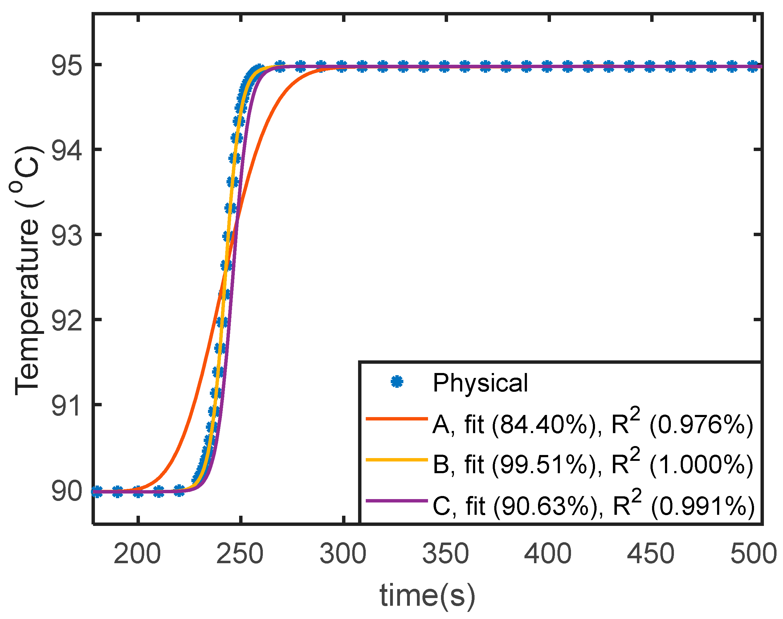
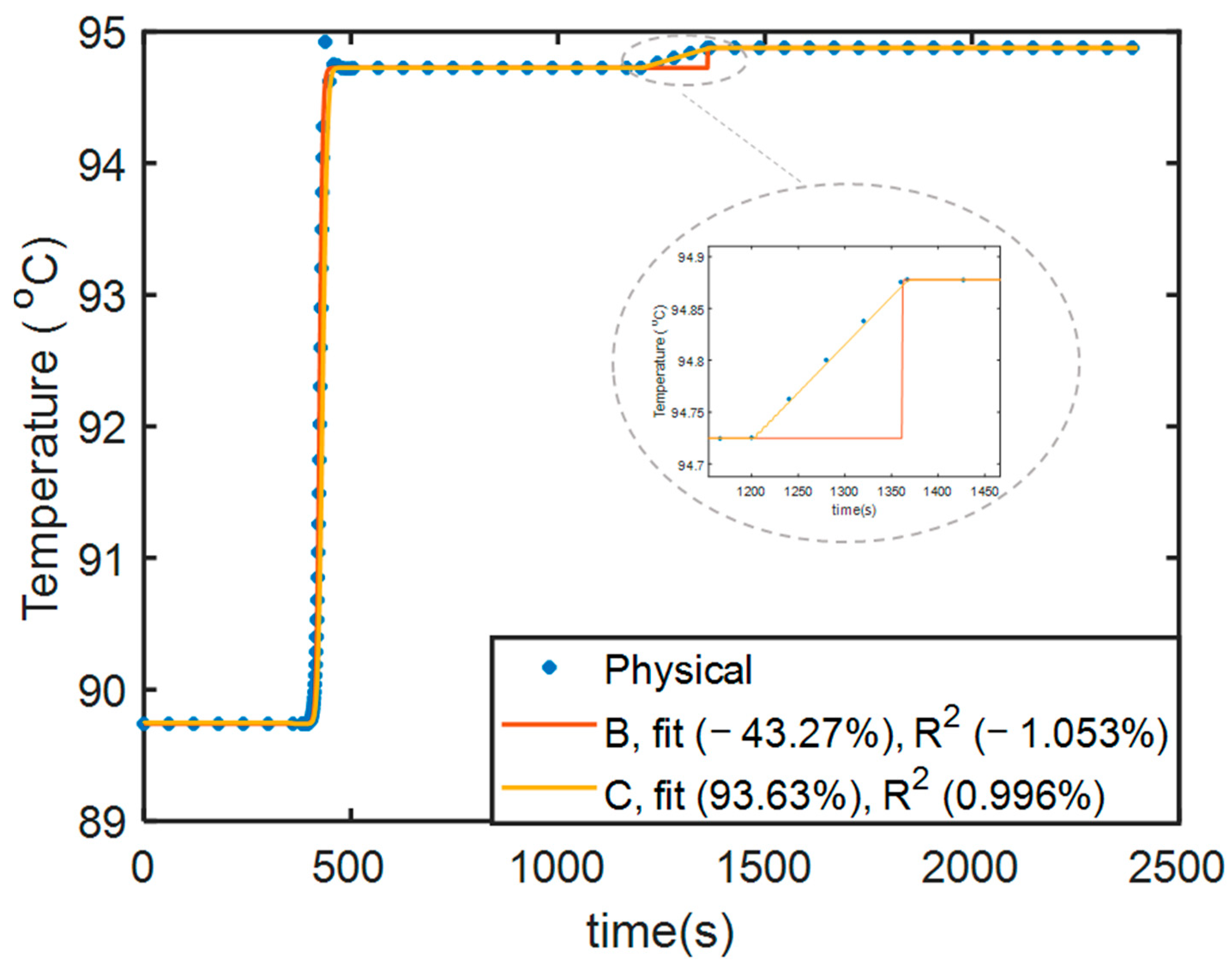
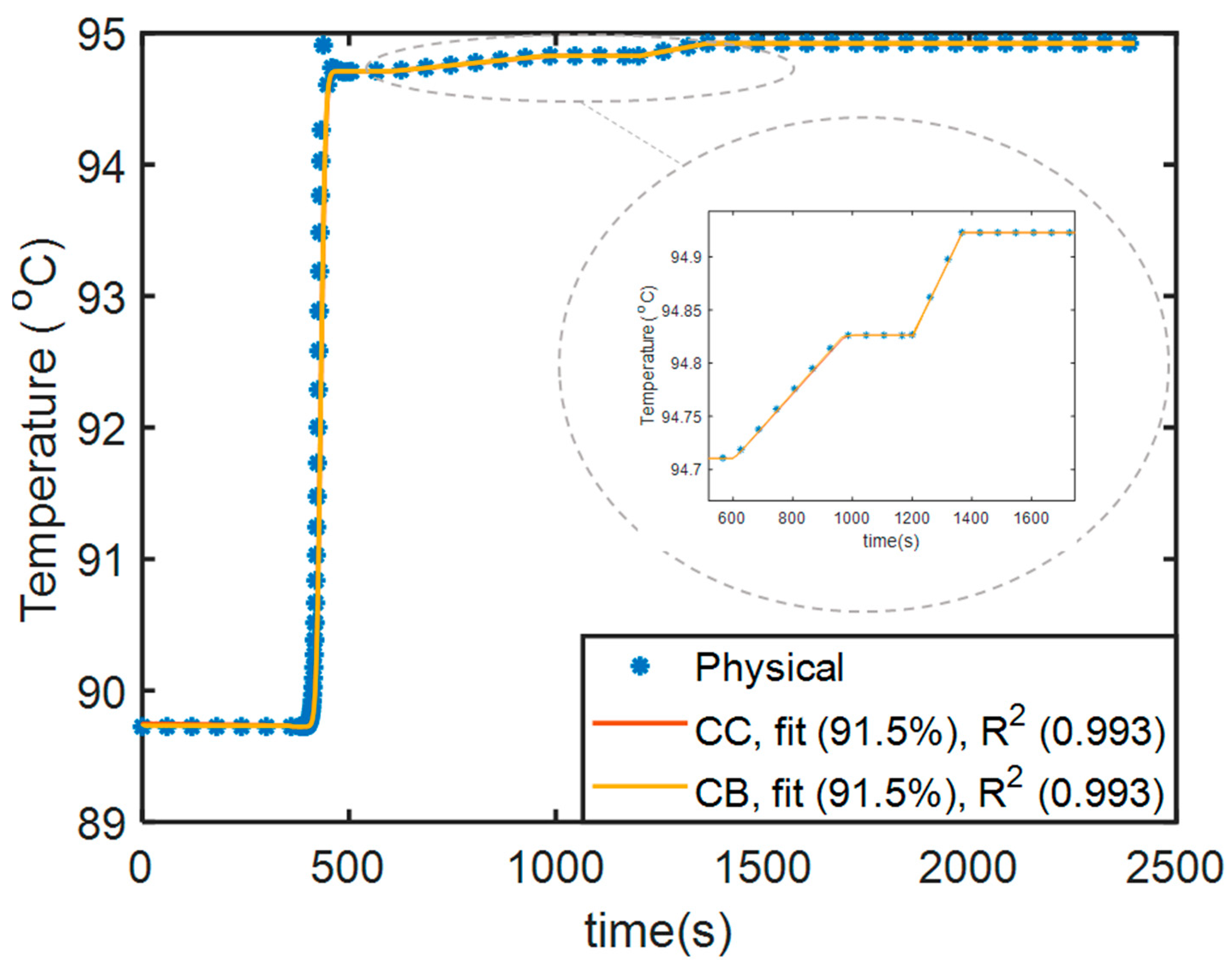
3. Model Validation Using DHN Simulation

To simulate a DHN, it is imperative to perform a degree of freedom (DOF) analysis to determine the number of variables that must be specified for the simulation. A presumed existing DHN is simulated in this research. Since the network is assumed to be pre-existing, the pipe dimensions, thermophysical properties of the pipe and water, and the pipe insulation properties are considered known parameters. The distribution pipes are represented as $k=\left\{mp, e{p}_{in},e{p}_{out},rp\right\}$, meaning that $nk=4$ for all DHNs, while the production pipes are represented as $p=\{pmp$, $prp\}$.

Thus, the degree of freedom can be calculated using the information in

Table 1. Degree of freedom (DOF) analysis of an existing DHN with a central generation station.

Variables	No. of Variables	Equations	No. of Equations
$T_{b,c,k,i}$	${\displaystyle {\displaystyle \sum }_{b=1}^{nb}}{\displaystyle {\displaystyle \sum }_{c=1}^{n{c}_b}}{\displaystyle {\displaystyle \sum }_{k=1}^{nk}}n{d}_{b,c,k}$	Discretised pipe equations	${\displaystyle {\displaystyle \sum }_{b=1}^{nb}}{\displaystyle {\displaystyle \sum }_{c=1}^{n{c}_b}}{\displaystyle {\displaystyle \sum }_{k=1}^{nk}}n{d}_{b,c,k}-1$
$T_{p,i}$	$n{d}_{pmp}+n{d}_{prp}$		$n{d}_{pmp}+n{d}_{prp}-2$
$T_{soil}$	1
$P_{demand,c}$	$nc$	Substation	$2nc$
${\dot{m}}_{b,c,k}$	$nk\times nc$	Distribution splitters	${\displaystyle {\displaystyle \sum }_{b=1}^{n_b}}3(n{c}_b-1)$
		Splitter continuity	$2nb$
		Distribution mixers	${\displaystyle {\displaystyle \sum }_{b=1}^{n_b}}2(n{c}_b-1)$
		Mixer continuity	$2nb$
${\dot{m}}_p$	2	Production splitter	$nb+1$
		Production mixer	2
$P_{gen}$	1	Power production in the generation section	1
$N_{variables}$	$\left\{{{\displaystyle \sum }}_{b=1}^{nb}{\displaystyle \sum }_{c=1}^{n{c}_b}{\displaystyle \sum }_{k=1}^{nk}n{d}_{b,c,k}\right\}+n{d}_{pmp}+n{d}_{prp}+\left(nk+1\right)nc+4$	$N_{equations}$	$\left\{{{\displaystyle \sum }}_{b=1}^{nb}{\displaystyle \sum }_{c=1}^{n{c}_b}{\displaystyle \sum }_{k=1}^{nk}n{d}_{b,c,k}-1+{\displaystyle \sum }_{b=1}^{nb}5(n{c}_b-1)\right\}+n{d}_{pmp }+n{d}_{prp}+2nc+5nb+2$

as $DOF=N_{variables}-N_{equations}=2nknc+2-nc-5nb-{\displaystyle \sum }_{b=1}^{nb}5(n{c}_b-1)$ for an existing DHN with a central heat-generation station.

Let us perform a case study simulation of an existing DHN with two branches $nb=2$, five consumers in each branch $n{c}_1=5, n{c}_2=5$. So, $nc=10$. The pipe diameters and lengths in the network are given in

Table 2. Pipe diameters and lengths for the case study DHN simulation.

Consumer	${\mathbf{Ф}}_{\mathit{m}\mathit{p}}$ (in)	${\mathit{L}}_{\mathit{m}\mathit{p}}$ (m)	${\mathbf{Ф}}_{\mathit{e}\mathit{p}}$ (in)	${\mathit{L}}_{\mathit{e}\mathit{p}}$ (m)
C1	8.00	279.93	5.00	95.21
C2	6.00	720.07	4.00	150.00
C3	5.00	176.46	2.00	40.00
C4	5.00	124.69	3.50	30.00
C5	1.50	397.32	1.50	100.00
C6	10.00	190.01	5.00	25.00
C7	8.00	97.04	3.50	10.00
C8	6.00	268.79	3.00	90.20
C9	5.00	1280.60	3.00	200.00
C10	5.00	198.28	4.00	50.00
Production	12.00	200.00

.

The DOF of the case study DHN simulation is $DOF=22$. This implies that twenty-two variables must be specified to simulate the DHN. The profiles of these variables must be defined as functions of time. This research uses the supply mass flow rates ${\dot{m}}_{c,k}$ (10 variables) of consumer component $c$, the power demands $P_{demand,c}$ (10 variables) of consumer component $c$, the soil temperature $T_{soil}$ (1 variable), and the plant generation temperature $T_{pmp,0}$ (1 variable). These declared variables are the simulation input variables, and their time profiles are shown in Figure 14, Figure 15 and Figure 16. The power demand profile and soil temperature were sourced from [26,27], respectively. The mass flow rate, adapted from [27], was modified to stay within the pipes’ maximum allowable limits to prevent erosion. A second-degree polynomial function was arbitrarily chosen for plant generation temperature to test the grey-box model under varying plant temperature conditions.

The simulation environment consists of MATLAB for the physical model and Simulink for the grey-box model, covering a duration of 1 to 24 h. The pipes in the DHN are discretised using an initial discretised segment length of $\Delta x_{initial}=$ 0.5 m and $\Delta x_{intial}=$ 8 m for the physical and grey-box models, respectively. The number of discretised segments of each pipe is initially calculated with the $\Delta x_{intial}$ using the piecewise functions in $\left(46\right)$ and $\left(47\right)$ for the physical and grey-box model simulations, respectively. Different piecewise functions are employed due to the distinct discretisation techniques used in the physical and grey-box models. In the grey-box model, the pipe inlet temperatures are treated directly as input variables, necessitating at least one discretised point to estimate the pipe outlet temperatures. Conversely, a second-order discretisation is applied to the spatial domain of the physical model, requiring a minimum of three discretisation points (including the inlet temperature) to estimate the pipe outlet temperatures. To ensure that a pipe is evenly discretised along its length, the discretised segment length of a pipe $pk$ to be used in the simulation is recalculated using $\Delta x_{pk}={\displaystyle \frac{L_{pk}}{n_{pk}-1}}$ and $\Delta x_{pk}={\displaystyle \frac{L_{pk}}{N_{pk}}}$ for the physical and grey-box model simulations, respectively. Consequently, $\Delta x_{pk}$ varies with the pipe lengths. However, the initially assigned segment lengths $\Delta x_{intial}$ are still referenced when describing the DHN simulation setup.

$$n_{pk}=\left\{\begin{array}{c}3 if round\left({\displaystyle \frac{L_{pk}}{\Delta x_{initial}}}\right)+1<3 \\ round\left({\displaystyle \frac{L_{pk}}{\Delta x_{initial}}}\right)+1 \left(\mathrm{includes} \mathrm{pipe} \mathrm{inlet} \mathrm{temperature}\right), otherwise \end{array}\right.$$

(46)

$$N_{pk}=\left\{\begin{array}{c}1 if round\left({\displaystyle \frac{L_{pk}}{\Delta x_{initial}}}\right)=0 \\ round\left({\displaystyle \frac{L_{pk}}{\Delta x_{initial}}}\right) otherwise\end{array}\right.$$

(47)

The physical model uses the ode15s solver in MATLAB, a variable-step, variable-order algorithm, with a maximum time step of 10 s and a relative and absolute tolerance of 1 × ${10}^{-4}$ and 1 × ${10}^{-6}$, respectively. Higher maximum time steps led to unrealistic simulation results, so the maximum time step was constrained to 10 s. Also, the Jacobian sparsity was supplied to the ode15s solver to hasten the simulation. The grey-box model in Simulink uses the fixed-step ode3 solver, based on the Bogacki–Shampine algorithm, with a fixed time step of 1 s.

The network temperatures after simulation are shown in Figure 17, Figure 18, Figure 19, Figure 20, Figure 21, Figure 22, Figure 23 and Figure 24. The physical model simulation results are represented with continuous lines, while the grey-box model simulation results are represented with asterisks. The DHN grey-box model achieves minimum and average ${R^2}_{DHN}$ values of 0.9983 and 0.9997 using $\left(48\right)$ and $\left(49\right)$, with corresponding minimum and average percentage fits of 95.92% and 98.64% using $\left(50\right)$ and $\left(51\right)$, respectively, when compared with the physical model. These results demonstrate the robustness of the grey-box LPV pipe model in capturing pipe dynamics without numerical issues.

$$minimum {R^2}_{DHN}=\min \left\{{R^2}_1, {R^2}_2, \dots , {R^2}_{npk}\right\}$$

(48)

$$average {R^2}_{DHN}={\displaystyle \frac{{{\displaystyle \sum }}_{pk}^{npk}{R^2}_{pk}}{npk}}$$

(49)

$$minimum \% fi{t}_{DHN}=\min \left\{\% fi{t}_1, \% fi{t}_2, \dots , \% fi{t}_{npk}\right\}$$

(50)

$$average \% fi{t}_{DHN}={\displaystyle \frac{{{\displaystyle \sum }}_{pk}^{npk}\% fi{t}_{pk}}{npk}}$$

(51)

Simulating the DHN with the physical model took approximately 165.9 min for a pipe segment length $\Delta x$ of 0.5 m with a maximum Courant number of 30.5 compared with 3.2 min with the grey-box model, which had a maximum Courant number of 0.19 and a maximum integration time step of 1 s, making the grey-box model about 52 times faster.

The DHN model validation results may seem counterintuitive, as the average percentage fit is higher for the DHN (with multiple pipes) case than for the single-pipe model. However, this discrepancy arises from the differing validation conditions. The single-pipe model was tested under strict conditions, including step changes in mass flow rate (50 $\mathrm{kg}/\mathrm{s}$) and soil temperature (40 °C), along with a pseudo-step change of 5 °C in inlet temperature. In contrast, the DHN validation involved smoothly varying profiles for input variables such as supply mass flow rates, power demands, plant temperature, and soil temperature.

Up to this point in the paper, the accuracy of the model simulations has been assessed based on the physical time delay, which is the time it takes for a fluid particle to travel from the pipe inlet to the outlet. This rationale led to the simulation of the physical and grey-box models using discretised pipe segment lengths $\Delta x_{intial}$ of 0.5 m and 7.14 m, respectively. However, a key question arises: could larger discretised pipe segment lengths achieve nearly the same accuracy as the high-fidelity physical model (simulated with $\Delta x_{intial}=0.5 \mathrm{m}$)? To investigate this, the physical and grey-box models are simulated at several $\Delta x_{intial}$ values and compared with the high-fidelity physical model, as shown in

Table 3. Computation time and fits for physical model simulated at varying $\Delta x$ values.

$\Delta x_{intial}$ (m)	1	2	5	8	10	15
Computation time (s)	24.03 $\times$ 60	3.72 $\times$ 60	29.92	8.36	4.31	2.26
Minimum $\% fi{t}_{DHN}$ (%)	99.97	99.91	99.83	99.7	99.66	99.50
Minimum ${R^2}_{DHN}$	1.0000	1.0000	1.000	1.000	1.000	1.000
Average $\% fi{t}_{DHN}$ (%)	99.99	99.98	99.95	99.92	99.90	99.86
Average ${R^2}_{DHN}$	1.0000	1.0000	1.000	1.000	1.000	1.000
Maximum integration time step (s)	10	10	10	10	10	10
Maximum $\mathrm{Co}$	15.25	7.71	3.05	2.46	2.46	2.46
$\Delta x_{intial}$ (m)	20	50	100	150	200	500
Computation time (s)	1.82	0.99	0.83	0.81	0.79	0.78
Minimum $\% fi{t}_{DHN}$ (%)	99.34	98.08	95.34	92.32	88.79	82.38
Minimum ${R^2}_{DHN}$	1.000	1.000	0.998	0.994	0.987	0.967
Average $\% fi{t}_{DHN}$ (%)	99.82	99.56	99.10	98.75	98.39	97.71
Average ${R^2}_{DHN}$	1.000	1.000	1.000	0.999	0.999	0.998
Maximum integration time step (s)	10	10	10	10	10	10
Maximum $\mathrm{Co}$	2.46	2.46	2.46	2.46	2.46	2.46

and

Table 4. Computation time and fits for grey-box model simulated at varying $\Delta x$ values.

$\Delta x_{intial}$ (m)	8	10	15	20	50	100	150	200	500
Computation time (s)	43.13	26.73	11.23	9.38	6.37	2.89	2.71	2.67	2.34
Minimum $\% fi{t}_{DHN}$ (%)	95.23	94.98	95.00	95.18	92.13	85.97	85.59	79.48	40.23
Minimum ${R^2}_{DHN}$	0.998	0.998	0.998	0.998	0.994	0.980	0.979	0.958	0.643
Average $\% fi{t}_{DHN}$ (%)	98.54	98.54	98.43	98.43	97.56	95.79	95.04	92.32	75.87
Average ${R^2}_{DHN}$	1.000	1.000	1.000	1.000	0.999	0.997	0.996	0.991	0.913
Maximum integration time step	58.18	66.93	90.76	142.78	343.38	523.66	731.72	907.81	1004.31
Maximum $\mathrm{Co}$	6.04	8.15	6.17	7.09	12.53	32.28	59.18	51.94	77.43

, using the ${R^2}_{DHN}$ in $\left(48\right)$ and $\left(49\right)$ and the percentage fit formula in $\left(50\right)$ and $\left(51\right)$.

The simulation solver of the grey-box model in Simulink is changed to ode15s, similar to the physical model, with a relative tolerance of 1 × ${10}^{-3}$ and with the Jacobian method being set to sparse analytical.

For all simulations in Table 3 and Table 4, the maximum velocity remains constant at 1.53 $\mathrm{m}/\mathrm{s}$ due to the identical mass flow rate profiles. The Courant numbers are calculated using $\left(52\right)$,

$$\mathrm{Co}=u_f\Delta t/\Delta x_{pk}$$

(52)

where $u_f$ is the fluid velocity and $\Delta t$ is the variable integration time step.

The maximum Courant numbers reported in Table 3 and Table 4 are determined by taking the maximum of all Courant numbers throughout the simulation. These values may not match the product of the maximum velocity and maximum time step divided by the pipe segment length. The Courant numbers exceed 1 due to the implicit integration methods employed by the numerical differentiation formula of the ode15s solver. Additionally, the minimum Courant number for all simulations is zero, as the integration time step at the initial condition is always zero.

From Table 3 and Table 4, it can be inferred that the simulation results of the low-fidelity physical model (obtained by simulating the physical model at an initial pipe segment length greater than $\Delta x_{intial}=0.5 \mathrm{m}$) consistently outperform the grey-box models in terms of fit to the high-fidelity physical model. This is reflected in the relatively high $\% fi{t}_{DHN}$ and ${R^2}_{DHN}$ values regardless of the initial pipe segment length $\Delta x_{intial}$. Moreover, the low-fidelity physical model simulations are consistently faster, demonstrating higher precision compared with the grey-box model.

The low-fidelity physical model with $\Delta x_{intial}=50 \mathrm{m}$ is recommended for future optimisation, as it achieves an average fit of 99.56% to the high-fidelity model with an ${R^2}_{DHN}$ value of 1. Additionally, the reduction in computation time for simulations with $\Delta x_{intial}>50 \mathrm{m}$ is relatively small when compared with the $\Delta x_{initial}=50 \mathrm{m}$. By the same criteria, the grey-box model with $\Delta x_{initial}=50 \mathrm{m}$ can also be used for future optimisation.

Although the low-fidelity physical model proves to be faster and more precise than the grey-box model, it is still essential to perform optimisation with both models to determine the best one. The reason for this is that the nature of an optimisation model influences the optimisation result, particularly with regard to local minima. In this case, the differing characteristics of the physical and grey-box models may present an opportunity to explore the advantages offered by each.

Finally, the simulation time in this paper was measured using MATLAB’s tic-toc function, which may differ from the actual CPU time. However, to minimise external influences, all non-MATLAB and Simulink activities on the laptop were closed before running the simulations. Additionally, each simulation case was executed three times to ensure accurate computation time measurement.

4. Conclusions

This study addressed the challenge of optimising district heating networks (DHNs) by developing a computationally efficient grey-box model suitable for dynamic real-time optimisation (DRTO). Unlike traditional physical models, which are accurate but computationally expensive, and black-box models, which lack extrapolation ability, the proposed grey-box linear parameter varying (LPV) pipe model balances accuracy and efficiency. The LPV pipe model was modified to allow DHN simulations with continuous mass flow rate profiles, expressing pipe outlet temperature as a function of inlet and soil temperatures, varying model parameters (dependent on mass flow rate), and constant parameters (determined through grid-search optimisation). Validation against a high-fidelity physical model (small discretisation) for a single pipe showed a 91.5% fit with an $R^2$ of 0.993 while being 5 times faster. Further validation in a 10-consumer DHN demonstrated an average fit of 98.64% and an $R^2$ of 0.9997, with the grey-box model running approximately 52 times faster than the physical model. Low-fidelity physical models (LFPMs), developed by increasing pipe segment lengths, remained more accurate and computationally efficient than the grey-box model when validated against the high-fidelity reference. Given the structural differences between grey-box and physical models, optimisation must be performed with both to determine which identifies better local minima. This research provides a foundation for future studies on DRTO implementation, exploring trade-offs between model accuracy, computational cost, and optimisation performance.

References

1. IEA Report. Heat—Renewables 2023—Analysis—IEA. Available online: https://www.iea.org/reports/renewables-2023/heat (accessed on 12 November 2024).
2. Pezzini, P.; Gomis-Bellmunt, O.; Sudrià-Andreu, A. Optimization techniques to improve energy efficiency in power systems. Renew. Sustain. Energy Rev. 2011, 15, 2028–2041. [Google Scholar] [CrossRef]
3. Rafati, A.; Shaker, H.R. Predictive maintenance of district heating networks: A comprehensive review of methods and challenges. Therm. Sci. Eng. Prog. 2024, 53, 102722. [Google Scholar] [CrossRef]
4. Jiang, M.; Rindt, C.; Smeulders, D.M.J. Optimal Planning of Future District Heating Systems—A Review. Energies 2022, 15, 7160. [Google Scholar] [CrossRef]
5. Untrau, A.; Sochard, S.; Marias, F.; Reneaume, J.-M.; Le Roux, G.A.; Serra, S. Analysis and future perspectives for the application of Dynamic Real-Time Optimization to solar thermal plants: A review. Sol. Energy 2022, 241, 275–291. [Google Scholar] [CrossRef]
6. Ellis, M.; Durand, H.; Christofides, P.D. A tutorial review of economic model predictive control methods. J. Process. Control. 2014, 24, 1156–1178. [Google Scholar] [CrossRef]
7. Hotvedt, M.; Hauger, S.O.; Gjertsen, F.; Imsland, L. Dynamic real-time optimisation of a CO2 capture facility. IFAC-PapersOnLine 2019, 52, 856–861. [Google Scholar] [CrossRef]
8. Untrau, A.; Sochard, S.; Marias, F.; Reneaume, J.-M.; Le Roux, G.A.; Serra, S. Dynamic Real-Time Optimization of a solar thermal plant during daytime. Comput. Chem. Eng. 2023, 172, 108184. [Google Scholar] [CrossRef]
9. Serasinghe, R.; Long, N.; Clark, J.D. Parameter identification methods for low-order gray box building energy models: A critical review. Energy Build. 2024, 311, 114123. [Google Scholar] [CrossRef]
10. Agner, F.; Kergus, P.; Pates, R.; Rantzer, A. Hydraulic Parameter Estimation in District Heating Networks. IFAC-PapersOnLine 2023, 56, 5438–5443. [Google Scholar] [CrossRef]
11. Wang, J.; Kong, F.; Pan, B.; Zheng, J.; Xue, P.; Sun, C.; Qi, C. Low-order gray-box modeling of heating buildings and the progressive dimension reduction identification of uncertain model parameters. Energy 2024, 294, 130812. [Google Scholar] [CrossRef]
12. Chen, Y.; Guo, M.; Chen, Z.; Chen, Z.; Ji, Y. Physical energy and data-driven models in building energy prediction: A review. Energy Rep. 2022, 8, 2656–2671. [Google Scholar] [CrossRef]
13. Bacher, P.; Madsen, H.; Perers, B. Models of the Heat Dynamics of Solar Collectors for Performance Testing. In Proceedings of the ISES Solar World Congress 2011, Kassel, Germany, 28 August–2 September 2011; Available online: www.imm.dtu.dk (accessed on 12 November 2024).
14. Nova-Rincon, A.; Sochard, S.; Serra, S.; Reneaume, J.-M. Dynamic simulation and optimal operation of district cooling networks via 2D orthogonal collocation. Energy Convers. Manag. 2020, 207, 112505. [Google Scholar] [CrossRef]
15. Li, Y.; O’Neill, Z.; Zhang, L.; Chen, J.; Im, P.; DeGraw, J. Grey-box modeling and application for building energy simulations—A critical review. Renew. Sustain. Energy Rev. 2021, 146, 111174. [Google Scholar] [CrossRef]
16. Thilker, C.A.; Bacher, P.; Bergsteinsson, H.G.; Junker, R.G.; Cali, D.; Madsen, H. Non-linear grey-box modelling for heat dynamics of buildings. Energy Build. 2021, 252, 111457. [Google Scholar] [CrossRef]
17. Svensen, J.L.; Bergsteinsson, H.G.; Madsen, H. Modeling and nonlinear predictive control of solar thermal systems in district heating. Heliyon 2024, 10, e31027. [Google Scholar] [CrossRef]
18. Blomgren, E.; D’ettorre, F.; Samuelsson, O.; Banaei, M.; Ebrahimy, R.; Rasmussen, M.; Nielsen, N.; Larsen, A.; Madsen, H. Grey-box modeling for hot-spot temperature prediction of oil-immersed transformers in power distribution networks. Sustain. Energy Grids Networks 2023, 34, 101048. [Google Scholar] [CrossRef]
19. Mercere, G.; Palsson, H.; Poinot, T. Continuous-time linear parameter-varying identification of a cross flow heat exchanger: A local approach. IEEE Trans. Control. Syst. Technol. 2011, 19, 64–76. [Google Scholar] [CrossRef]
20. Chouaba, S.E.; Chamroo, A.; Ouvrard, R.; Poinot, T. A counter flow water to oil heat exchanger: MISO quasi linear parameter varying modeling and identification. Simul. Model. Pract. Theory 2012, 23, 87–98. [Google Scholar] [CrossRef]
21. Naspolini, A.; Morato, M.M.; Flesch, R.C.C.; Normey-Rico, J.E. Enhanced gas-lift system operation using LPV nonlinear model predictive control. Geoenergy Sci. Eng. 2024, 239, 212969. [Google Scholar] [CrossRef]
22. Boutourda, F.; Ouvrard, R.; Poinot, T.; Mehdi, D.; Mesquine, F.; De Tredern, E.; Jauzein, V. A global approach to estimate continuous-time LPV models for wastewater nitrification. IFAC-PapersOnLine 2024, 58, 61–66. [Google Scholar] [CrossRef]
23. Shayan, M.E.; Petrollese, M.; Rouhani, S.H.; Mobayen, S.; Zhilenkov, A.; Su, C.L. An innovative two-stage machine learning-based adaptive robust unit commitment strategy for addressing uncertainty in renewable energy systems. Int. J. Electr. Power Energy Syst. 2024, 160, 110087. [Google Scholar] [CrossRef]
24. The Engineering ToolBox. Water—Specific Heat vs. Temperature. Available online: https://www.engineeringtoolbox.com/specific-heat-capacity-water-d_660.html (accessed on 13 January 2025).
25. Duquette, J.; Rowe, A.; Wild, P. Thermal performance of a steady state physical pipe model for simulating district heating grids with variable flow. Appl. Energy 2016, 178, 383–393. [Google Scholar] [CrossRef]
26. Elhafaia, M.H.; Nova-Rincon, A.; Sochard, S.; Serra, S.; Reneaume, J.-M. Optimization of the pipe diameters and the dynamic operation of a district heating network using a robust initialization strategy. Appl. Therm. Eng. 2025, 258, 124533. [Google Scholar] [CrossRef]
27. Tijani, O.E.; Serra, S.; Sochard, S.; Viot, H.; Henon, A.; Malti, R.; Lanusse, P.; Reneaume, J.M. Transient Modelling and Simulation for Optimal Future Management of a District Heating Network. 31ème Congrès Français Therm 2023. [Google Scholar] [CrossRef]
28. ThermExcel. Physical Characteristics of Water. 2003. Available online: https://www.thermexcel.com/english/tables/eau_atm.htm (accessed on 14 November 2024).
29. The Engineering ToolBox. Water—Thermal Conductivity vs. Temperature. Available online: https://www.engineeringtoolbox.com/water-liquid-gas-thermal-conductivity-temperature-pressure-d_2012.html (accessed on 14 November 2024).
30. Bergman, T.L.; Lavine, A.S.; Incropera, F.P.; Dewitt, D.P. Fundamentals of Heat and Mass Transfer, 7th ed.; John Wiley & Sons: Hoboken, NJ, USA, 2011. [Google Scholar]
Figure 1. A district heating network with a single generation station, multiple branches, and no thermal storage.
Energies 18 01626 g001
Figure 2. The generation section of a DHN.
Energies 18 01626 g002
Figure 3. The modelling of a consumer component c in branch b of a DHN distribution section.
Energies 18 01626 g003
Figure 4. The cross-sectional view of a pipe carrying hot fluid.
Energies 18 01626 g004
Figure 5. LPV model for outlet temperature as a function of inlet temperature for β = 0 ,   α = 1 ,   T d = 0 —Model A.
Energies 18 01626 g005
Figure 6. LPV model for outlet temperature as a function of inlet temperature for β = 0 ,   α = 0 ,   T d   0 —Model B.
Energies 18 01626 g006
Figure 7. LPV model for outlet temperature as a function of inlet temperature for β = 0 ,   α = 1 ,   T d 0 —Model C.
Energies 18 01626 g007
Figure 8. Outlet pipe temperatures for inlet temperature variation.
Energies 18 01626 g008
Figure 9. Simulink representation of model B.
Energies 18 01626 g009
Figure 10. Simulink representation of model C.
Energies 18 01626 g010
Figure 11. Outlet pipe temperatures for inlet temperature variation and mass flow rate excitation.
Energies 18 01626 g011
Figure 12. Distributed delay for the soil temperature influence on the pipe outlet temperature.
Energies 18 01626 g012
Figure 13. Pipe outlet temperature for input variable variations.
Energies 18 01626 g013
Figure 14. Supply mass flow rates of the consumers.
Energies 18 01626 g014
Figure 15. Plant generation and soil temperatures.
Energies 18 01626 g015
Figure 16. Power demands of the consumers.
Energies 18 01626 g016
Figure 17. Main pipe outlet temperatures for consumers 1–5 and production.
Energies 18 01626 g017
Figure 18. Main pipe outlet temperatures for consumers 6–10.
Energies 18 01626 g018
Figure 19. Extended-in pipe outlet temperatures for consumers 1–5.
Energies 18 01626 g019
Figure 20. Extended-in pipe outlet temperatures for consumers 6–10.
Energies 18 01626 g020
Figure 21. Extended-out pipe outlet temperatures for consumers 1–5.
Energies 18 01626 g021
Figure 22. Extended-out pipe outlet temperatures for consumers 6–10.
Energies 18 01626 g022
Figure 23. Return pipe outlet temperatures for consumers 1–5.
Energies 18 01626 g023
Figure 24. Return pipe outlet temperatures for consumers 6–10 and production.
Energies 18 01626 g024