Two-Level Optimal Scheduling of Electric–Aluminum–Carbon Energy System Considering Operational Safety of Electrolytic Aluminum Plants

Abstract

In recent years, the mounting pressure on the integration of renewable power has emerged as a crucial concern within renewable power systems. This situation urgently necessitates an enhancement in the operational flexibility of the demand side. As an energy-intensive load, electrolytic aluminum plants have great potential to participate in the demand response. However, existing models for electrolytic aluminum load regulation lack verification of operational safety, and there is a lack of consideration of carbon trading mechanisms. To this end, this paper proposes a two-level optimization framework for electric–aluminum–carbon energy systems. More specifically, this work presents a safety-constrained electrolytic aluminum plant model, which considers operational states swinging with key parameters and limitations verified by the thermal dynamic simulations of electrolytic aluminum electrolyzers. In addition, green certificate and tiered carbon trading mechanisms are both introduced to the electric–aluminum–carbon energy. Case studies show that the proposed framework can significantly reduce the system emission by 21.9%, improve the overall economic efficiency by 16.5%, and increase the renewable integration rate by 4.5%, with an additional 8.6% of carbon reduction that can be achieved by adopting EU carbon price policies.

1. Introduction

In recent years, the installed capacity of renewable generation has been on a continuous upward trajectory. It is estimated that, by 2025, wind and solar generation in China will account for over 35% of the total installed capacity [1]. However, frequent curtailment of renewable power persists in specific regions, with the Northwest China region still experiencing a wind curtailment rate of 5.7% in 2024 [2]. The structural imbalance between the rapid growth of renewable generation and the grid integration capability has become increasingly pronounced [3]. To address these challenges, it is imperative to coordinate between electricity, ancillary service, and carbon markets, thereby ensuring the flexible and low-carbon operation of renewable energy systems [4].

The intermittent nature of renewable energy heightens the need for flexible regulation, i.e., converting the surplus of renewable electricity to other types of the energy (e.g., hydrogen [5], heat [6], or chemical products such as aluminum [7]) and discharging them at a different times. An electrolytic aluminum load, as a significant industrial load in China, is characterized by high energy consumption, with the capacity of a single electrolytic aluminum plant reaching several hundred megawatts [8], making them have great potential for participation in demand response. Nevertheless, their operation flexibility has not yet been fully explored. This is because, as an energy-intensive chemical plant, practical electrolytic aluminum plants adhere to the traditional operational principle—“safety, stability, long-term, full-capacity, and high-quality operation” [9]. Their yield production and power consumption are less likely to change, as both increasing and decreasing the production rate could potentially break the thermal balance of a plant and cause permanent damage [10].

However, continuously rising raw material prices, increasingly stringent carbon emission standards, and the growing share of renewable energy pose challenges to the electrolytic aluminum industry [11]. Utilizing renewable energy for flexible production is a crucial means of maintaining competitiveness in the electrolytic aluminum industry [12]. However, existing electrolytic aluminum load regulation strategies fail to fully capture the operational flexibility and carbon trading incentive mechanisms under renewable energy systems.

There have been studies that have investigated the demand response potential of electrolytic aluminum plants within renewable power systems. For example, refs. [7,13] modeled an electrolytic aluminum load by constraining its aggregate input power over a certain period. Ref. [14] modeled an electrolytic aluminum load as regular curtailable load with curtailment penalties. Ref. [15] explored the power shifting characteristics of an electrolytic aluminum load with respect to the production rate. Refs. [16,17,18] investigated the equivalent electric circuit model for the dynamic response of electrolytic aluminum plants, which facilitates their participation in frequency regulation. In [19,20], multiple operational states of electrolytic aluminum loads were defined, and the operational limits of electrolytic aluminum loads were considered by constraining the number of the operational states/regulations that occurred over the day. The above models have posed constraints for electrolytic aluminum loads in multiple dimensions, i.e., day-ahead operational limits, state shifting, and power dynamics. However, the effectiveness of the above models in ensuring the operational safety for practical plants has not been verified. A detailed comparison of previous works is shown in

Table 1. Previous studies on modeling electrolytic aluminum load in power and energy systems.

Reference	Modeling Type	Operational Safety Modeling
[7]	Continuous model	Aggregate input power constraints
[13]	Continuous model	Aggregate input power constraints
[14]	Continuous model	No
[15]	Continuous model	No
[16]	Electric circuit (power dynamic)	No
[17]	Electric circuit (power dynamic)	No
[18]	Electric circuit (power dynamic)	No
[19]	Multi-stage model	State occurrence constraints
[20]	Multi-stage model	Regulation occurrence constraints
This work	Multi-stage model	Safety constraints verified by thermal dynamics

.

Furthermore, as a carbon-intensive load, an electrolytic aluminum plant will face complex and tough carbon policies. There have been studies that investigated the integration of different carbon trading mechanisms within power system optimization problems. For example, ref. [21] established a low-carbon power system dispatch model based on a tiered carbon trading mechanism. Refs. [22,23] and further introduced tiered carbon trading mechanisms for electric vehicles. Ref. [24] proposed a green certificate trading model for integrated energy systems. The electrolytic aluminum industry is a key target for carbon reduction that the Chinese government pays close attention to [25]. However, carbon trading mechanisms have not yet been fully considered in electrolytic aluminum energy systems. In this work, both green certificates and carbon trading are introduced to the electrolytic aluminum energy system.

This paper proposes a two-level optimization framework for electric–aluminum–carbon energy systems considering the safety-constrained aluminum production process. To be specific, this paper proposes a safety-constrained electrolytic aluminum plant model, which facilities it actively participating in the demand response while ensuring the operational safety of aluminum electrolyzers. The proposed aluminum plant model is established using thermal dynamic simulations, in which safety operational boundaries are evaluated based on a critical scenario analysis. Green certificate and tiered carbon trading mechanisms are introduced and analyzed. The proposed framework uses multiple linearization techniques and is formulated as mixed integer linear programming (MILP) models, which can be easily generalized and solved by commercial optimization solvers such as Gurobi or Cplex.

The main contributions of this paper are as follows:

(1)

This paper for the first time evaluates the safety operational boundaries of electrolytic aluminum loads by performing thermal dynamic simulations of aluminum electrolyzers. Based on that, a safety-constrained electrolytic aluminum plant model is presented. The model is formulated as MILP and can be easily adopted in energy system optimization problems.

(2)

This paper proposes a two-level economic dispatch framework for the electrolytic aluminum energy system. The framework transmits information between upper and lower levels and achieves mutual benefits for multiple stakeholders.

(3)

Carbon mechanisms are further considered within the optimal scheduling of the electrolytic aluminum load. The proposed framework introduces green certificate and tiered carbon trading mechanisms, while coordinating the optimization of electricity, aluminum, and carbon is achieved.

(4)

Case studies show that the proposed framework can significantly reduce the system emission by 21.9%, improve the overall economic efficiency by 16.5%, and increase the renewable integration rate by 4.5%, with an additional 8.6% of carbon reduction that be achieved by adopting EU carbon price policies.

2. Two-Level Optimization Framework

As energy-intensive enterprises, electrolytic aluminum companies consider their production data, output information, and finished product prices as corporate privacy. Therefore, they typically do not directly connect to the power system control center, and the power system cannot directly control the electrolytic aluminum load. The proposed two-level optimal dispatch framework decomposes the optimization problem into two subproblems for different stakeholders (e.g., the grid operator and electric aluminum plants in this work). The two-level structure may not achieve global optimality, but it is more practical, as each participant optimizes its own objectives (e.g., minimizing the generation cost or maximizing profit in this work) and shares only the necessary aggregated or reduced information with others.

As shown in Figure 1, the upper-level grid operator side optimizes power generation based on renewable power and regular load forecast considering green certificate trading. It then aggregates the surplus renewable and thermal power that can be supplied to the lower-level electrolytic aluminum plant. The lower-level electrolytic aluminum plant receives this information and optimizes the production and emission based on its own operational characteristic. Through the joint optimization of the power side and load side, the dispatch strategy ensures that the electrolytic aluminum enterprise gains economic and environmental benefits and increases the integration of renewable power at the same time.

3. Mathematical Model

3.1. Upper-Level Optimization Model

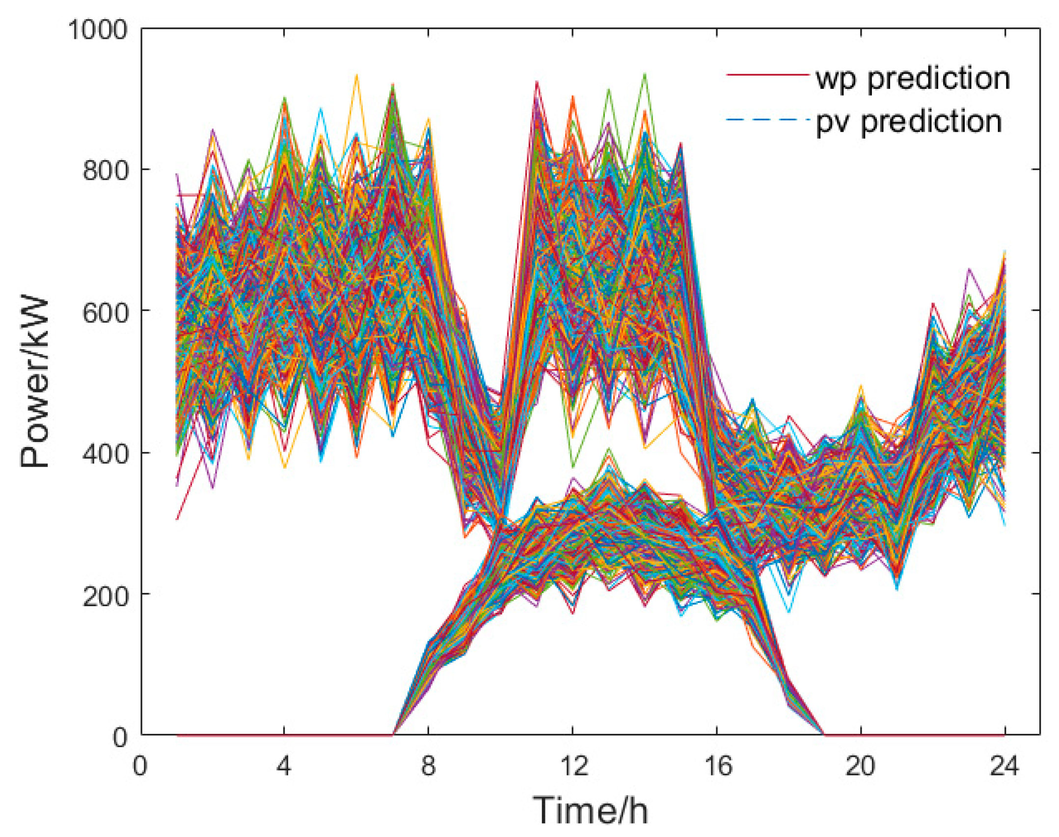
3.1.1. Renewable Generation Scenario Reduction

Renewable energy is difficult to predict. To accurately describe the random fluctuation characteristics of wind speed and solar radiation, this paper uses a scenario analysis approach to address the uncertainty of renewable generation. Based on historical data shown in Figure 2, the corresponding probability density functions of wind speed and solar radiation are established. It is assumed that wind power follows a normal distribution N(μ, σ²), where the expected value of wind power is μ and the fluctuation percentage is σ. The Latin hypercube sampling method is used to sample the cumulative distribution functions of wind speed and solar radiation, generating representative scenario sets for wind speed and solar intensity.

Then, the scenario reduction is implemented using the probability distance-based fast descendant elimination method with μ = 1 and σ = 0.12. The obtained renewable generation scenario distributions are shown in Figure 3.

3.1.2. Green Certificate Trading Mechanism

A green certificate is a certificate issued by the government to non-hydropower renewable energy generation enterprises. The number of certificates is related to the amount of renewable energy generated by the enterprise and is used to prove that the electricity produced by the enterprise originates from renewable energy, thus demonstrating its environmentally friendly attributes. The renewable energy quota specifies the proportion of renewable energy in the electricity generated or used by the enterprise. When the number of green certificates produced by a renewable energy generation enterprise exceeds the quota, the enterprise can sell the surplus certificates to make a profit. If the number is below the quota, the power plant must purchase green certificates. If an enterprise responsible for renewable energy integration exceeds its renewable energy absorption quota, it can sell the surplus green certificates in the market. On the other hand, if an electricity-consuming enterprise’s renewable energy integration is insufficient to meet its quota, it must purchase additional green certificates to fulfill the renewable energy integration targets. The green certificate trading mechanism not only encourages renewable energy enterprises to actively generate power and profit but also urges electricity-consuming enterprises to take responsibility for utilizing green electricity.

$$C_{GCT}=\left\{\begin{array}{l}{\lambda }_{buy}(P_q-P_{green})\hspace{1em}\hspace{1em}{P}_{green}<P_q\\ {\lambda }_{sale}(P_q-P_{green})\hspace{1em}\hspace{1em}{P}_{green}\ge P_q\end{array}\right.$$

(1)

where C_GCT represents the green certificate trading cost; λ_buy and λ_sale are the prices for purchasing and selling green certificates, respectively; and P_q and P_green represent the renewable energy integration quota and actual integration amount, respectively.

When P_green < P_q, the actual integration of renewable green electricity is less than the integration quota, and the enterprise needs to purchase green certificates. C_GCT is a positive value, indicating that the green certificate trading cost increases. When P_green ≥ P_q, the actual integration of renewable green electricity is not less than the integration quota, and the enterprise can sell green certificates. C_GCT is a negative value, indicating that the green certificate trading increases profit.

3.1.3. Upper-Level Constraints

To strengthen the argument for the validity of the proposed strategy, green certificate trading is considered in the objective function. The costs of green certificate are used to replace the wind and solar curtailment penalty costs. After considering the green certificate, the total system cost consists of the system operating cost and green certificate trading cost. The upper-level optimization model that considers the green certificate in the multi-energy complementary power system dispatch model is shown below:

$$\min F=C_{op}+C_{GCT,G}$$

(2)

$$C_{op}=C_g+C_w+C_{pv}$$

(3)

$$P_{green,t}=P_{w,t}+P_{pv,t}$$

(4)

$$C_g={\displaystyle \sum _{t=1}^T{\displaystyle \sum _{g=1}^{N_g}\left[a_g+b_g{P}_{g,t}+c_g{(P_{g,t})}^2\right]}}$$

(5)

$$C_w={\rho }_w{\displaystyle \sum _{t=1}^T{P}_{w,t}}$$

(6)

$$C_{pv}={\rho }_{pv}{\displaystyle \sum _{t=1}^T{P}_{pv,t}}$$

(7)

$$C_{GCT,G}=\left\{\begin{array}{l}{\lambda }_{buy}({\phi }_q{\displaystyle \sum _{t=1}^T{P}_{load,t}}-{\displaystyle \sum _{t=1}^T{P}_{green,t}})\hspace{1em}\hspace{1em}{\displaystyle \sum _{t=1}^T{P}_{green,t}}<{\phi }_q{\displaystyle \sum _{t=1}^T{P}_{load,t}}\\ {\lambda }_{sale}({\phi }_q{\displaystyle \sum _{t=1}^T{P}_{load,t}}-{\displaystyle \sum _{t=1}^T{P}_{green,t}})\hspace{1em}\hspace{1em}{\displaystyle \sum _{t=1}^T{P}_{green,t}}\ge {\phi }_q{\displaystyle \sum _{t=1}^T{P}_{load,t}}\end{array}\right.$$

(8)

where C_op represents the system operating cost and C_g, C_w, and C_pv represent the operating costs of thermal power units, wind farms, and photovoltaic power stations during the scheduling period. T is the scheduling period, which is set to 24 h in this paper; a_g, b_g, and c_g are the fuel cost coefficients for thermal power units; P_g,t represents the output power of thermal power unit i at time period t; N_g is the number of thermal power units involved in scheduling; ρ_w is the operating cost coefficient for the wind farm; N_w is the number of wind farms involved in scheduling; P_w,t represents the output power of wind farm at time period t; ρ_pv is the operating cost coefficient for the photovoltaic power station; N_pv is the number of photovoltaic power stations involved in scheduling; P_pv,t represents the output power of the photovoltaic power station at time period t; φ_q is the renewable energy quota coefficient; P_load,t is the forecasted load at time period t; and Δt represents the time interval for system scheduling, which is set to 1 h in this paper.

Equation (5) should be linearized to ensure the linearity of the model. Note that for any continuous function g(x), the following incremental linearization technic can be used:

$$g(x)=g(x_1)+{\displaystyle \sum _{k=1}^{NPL-1}[g(x_{k+1})-g(x_k)]\cdot {\delta }_k}$$

(9)

$$x=x_1+{\displaystyle \sum _{k=1}^{NPL-1}[x_{k+1}-x_k]\cdot {\delta }_k}$$

(10)

$$\begin{array}{cc}{\delta }_{k+1}\le {\eta }_k\le {\delta }_k& k=1,2,\dots NPL-2\end{array}$$

(11)

$$\begin{array}{cc}{\eta }_k\in \{0,1\},0\le {\delta }_k\le 1& k=1,2,\dots NPL-1\end{array}$$

(12)

where NPL is the number of interpolation points for piecewise linearization and η_k and δ_k are auxiliary variables.

Similarly, Equation (8) can be reformulated in a linear form as

$$C_{GCT}={\lambda }_{buy}\cdot {\chi }_{\mathrm{in},\mathrm{GCT}}-{\lambda }_{sale}\cdot {\chi }_{\mathrm{out},\mathrm{GCT}}$$

(13)

$${\chi }_{\mathrm{in},\mathrm{GCT}}-{\chi }_{\mathrm{out},\mathrm{GCT}}={\phi }_q{\displaystyle \sum _{t=1}^T{P}_{load}^t}-{\displaystyle \sum _{t=1}^T{P}_{green}^t}$$

(14)

$${\chi }_{\mathrm{in},\mathrm{GCT}},{\chi }_{\mathrm{out},\mathrm{GCT}}\ge 0$$

(15)

where χ_in,GCT and χ_out,GCT are auxiliary variables representing the insufficient or surplus portion of green electricity usage.

Furthermore, the ramping performance and on–off status of thermal generation plants should be constrained. Herein, the unit commitment model of thermal power plants is considered as per (16)–(25). Equations (16)–(20) limit the output power of the thermal unit at each time step; Equations (21)–(23) constrain the operational state of the thermal unit; and Equations (24) and (25) model the minimum operation period of each state.

$$\underset{¯}{P_{g.t}}\le P_{g.t}\le \overline{P_{g.t}}$$

(16)

$$\overline{P_{g.t}}\le P_{g,\max }[u_{g,t}-z_{g,t+1}]+S{D}_g{z}_{g,t+1}$$

(17)

$$\overline{P_{g.t}}\le P_{g.t-1}+{\mathrm{RU}}_g{u}_{g,t-1}+S{U}_g{y}_{g,t}$$

(18)

$$\underset{¯}{P_{g.t}}\ge P_{g,\min }{u}_{g,t}$$

(19)

$$\underset{¯}{P_{g.t}}\ge P_{g,t-1}-R{D}_g{u}_{g,t}-S{D}_g{z}_{g,t}$$

(20)

$$y_{g,t}-z_{g,t}=u_{g,t}-u_{g,t-1}$$

(21)

$$y_{g,t}+z_{g,t}\le 1$$

(22)

$$y_{g,t},z_{g,t},u_{g,t}=\{0,1\}$$

(23)

$$\begin{array}{cc}{\displaystyle \sum _{t=k_t}^{k_t+{\mathrm{UT}}_g-1}{u}_{g,t}\ge {\mathrm{UT}}_g\cdot y_{g,k_t}}& \forall k_t=1\dots T-{\mathrm{UT}}_g+1\end{array}$$

(24)

$$\begin{array}{cc}{\displaystyle \sum _{t=k_t}^{k_t+D{\mathrm{T}}_g-1}\left(1-u_{g,t}\right)\ge D{\mathrm{T}}_g\cdot z_{g,k}}& \forall k_t=1\dots T-{\mathrm{DT}}_g+1\end{array}$$

(25)

where k_t is the loop-back time index; k_t and t are aliases; u_g,t, y_g,t, and z_g,t are binary variables representing the generators’ operation sate, turn-on action, and shut-down action; UT_g and DT_g are the generators’ minimum-on and -off period; and RU_g, RD_g, SU_g, and SD_g are ramp up, ramp down, start up, and shut down power.

In addition, the renewable power generation (wind and solar) is modeled as

$$0\le P_{w,t}\le P_{w,\max }$$

(26)

$$0\le P_{pv,t}\le P_{pv,\max }$$

(27)

3.2. Lower-Level Optimization Model

3.2.1. Electrical Model of Aluminum Electrolyzers

An aluminum electrolyzer is connected by multiple cells and supplied by a DC current. The relationship between the voltage and current of an aluminum electrolyzer can be modeled as

$$U_{\mathrm{dc}}=I_{\mathrm{dc}}{R}_{\mathrm{as}}+E_{\mathrm{as}}$$

(28)

$$P_{\mathrm{AL}}=U_{\mathrm{dc}}{I}_{\mathrm{dc}}$$

(29)

where U_dc represents the DC voltage in the electrolyzer; I_dc represents the current passing through the electrolyzer; P_AL represents the power consumed by the electrolyzer; R_as represents the equivalent resistance of the electrolyzer; and E_as represents the back electromotive force of the electrolyzer.

The aluminum production rate–current relationship is

$$Y_{as}={\alpha }_{as}{I}_{dc}{\eta }_1{N}_{as}$$

(30)

where Y_as represents the aluminum production per unit time; α_as represents the electrochemical equivalent of aluminum; η₁ represents the electrolysis efficiency of the electrolytic aluminum load; and N_as represents the number of electrolytic cells.

When the electrolytic aluminum plant operates below the rated power, its efficiency is expressed as follows:

$${\eta }_1={\displaystyle \frac{I_{dc}{\eta }_{10}}{I_{dc0}}}$$

(31)

When the electrolytic aluminum plant operates above the rated power, its efficiency decreases, and the expression is as follows:

$${\eta }_1={\displaystyle \frac{I_{dc0}{\eta }_{10}}{I_{dc}}}$$

(32)

where I_dc0 represents the rated current of the electrolytic aluminum load DC bus and η_dc0 represents the rated electrolysis efficiency of the electrolytic aluminum load.

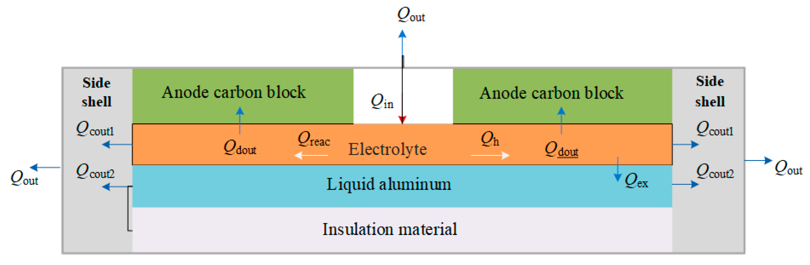
3.2.2. Thermal Dynamics of Aluminum Electrolyzers

To facilitate the analysis of the thermal characteristics of the aluminum electrolyzer, the thermal model of the aluminum electrolytic cell is divided into an electrolyte–aluminum system and a shell–carbon block system (see Figure 4).

Since the molten electrolyte and aluminum liquid are in a state of circulating flow, the temperatures of the electrolyte and aluminum liquid are assumed to be uniform. Therefore, the thermal balance equation of the electrolyte–aluminum system can be described as

$$Q_{\mathrm{in}}-Q_{\mathrm{reac}}-Q_{\mathrm{h}}-Q_{\mathrm{cout}1}-Q_{cout2}-Q_{\mathrm{dout}}=(c_e{m}_e+c_l{m}_l)\Delta T_e$$

(33)

where Q_in is the generated Joule heat; Q_reac is the heat consumed by the electrochemical reaction process; Q_h is raw material heating energy; Q_cout1 and Q_cout2 are the heat dissipated from electrolyte and aluminum; Q_dout is the heat dissipated to carbon blocks; c_e and c_s are the specific heat capacity of the electrolyte and liquid aluminum; m_e and m_l are the mass of the electrolyte and liquid aluminum; and ΔT_e is the temperature change of the electrolyte- aluminum system.

The shell–carbon block system is located between the external environment and the electrolyte–aluminum system. The heat inside the cell is dissipated into the outside air through the shell. The thermal balance equation of the shell–carbon block system can be described as

$$Q_{cout1}+Q_{cout2}+Q_{dout}-Q_{out}=c_s{m}_s\Delta T_s$$

(34)

where Q_out is the heat transferred from the shell–carbon block system to the environment; c_s and m_s are the specific heat capacity and mass of the shell–carbon block system; and ΔT_s is the temperature change of the shell–carbon block system.

The heat energy component in the above equations can be further expressed as

$$Q_{in}=(U_{cell}-E)I\Delta t$$

(35)

$$Q_{reac}=Y_{as}{E}_{\Delta H_r}\Delta t$$

(36)

$$Q_h=Y_{as}{E}_{\Delta H_h}\Delta t$$

(37)

$$Q_{cout1}=h_e(T_e-T_s)A_e\Delta t$$

(38)

$$Q_{cout2}=h_l(T_e-T_s)A_l\Delta t$$

(39)

$$Q_{dout}=h_c(T_e-T_s)A_c\Delta t$$

(40)

$$Q_{out}=h_s(T_s-T_a)A_s\Delta t$$

(41)

where h_e, h_l, h_c, and h_s are the convective heat transfer coefficient between the electrolyte and shell, liquid aluminum and shell, electrolyte and carbon blocks, and shell and carbon blocks; A_e, A_l, A_c, and A_s are heat transfer areas; ΔE_Hr and ΔE_Hs are the energy consumption of the electrochemical reaction and heating raw materials per unit of aluminum production; and T_a is the environmental temperature. Note that ΔE_Hs may vary depending on the target temperature.

By substituting (35)–(41) into (33) and (34), the overall thermal dynamics of aluminum cells can be written as

$${\displaystyle \frac{\partial T_e}{\partial t}}={\displaystyle \frac{(U_{cell}-E)I-Y_{as}(E_{\Delta H_r}+E_{\Delta H_h})}{c_e{m}_e+c_l{m}_l}}-{\displaystyle \frac{(h_e{A}_e+h_l{A}_l+h_c{A}_c)(T_e-T_s)}{c_e{m}_e+c_l{m}_l}}$$

(42)

$${\displaystyle \frac{\partial T_s}{\partial t}}={\displaystyle \frac{(h_e{A}_e+h_l{A}_l+h_c{A}_c)(T_e-T_s)}{c_s{m}_s}}-{\displaystyle \frac{h_s(T_s-T_a)A_s}{c_s{m}_s}}$$

(43)

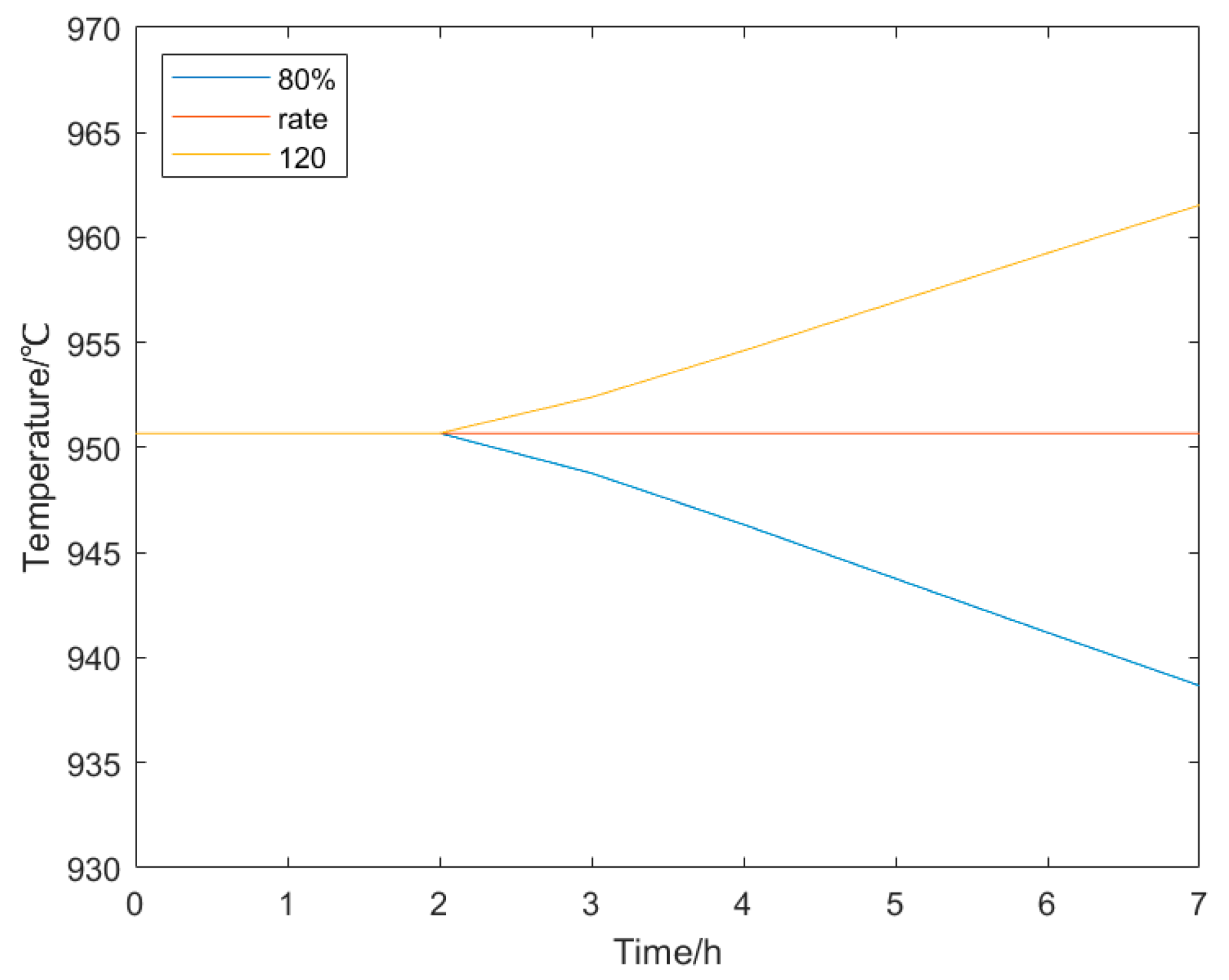
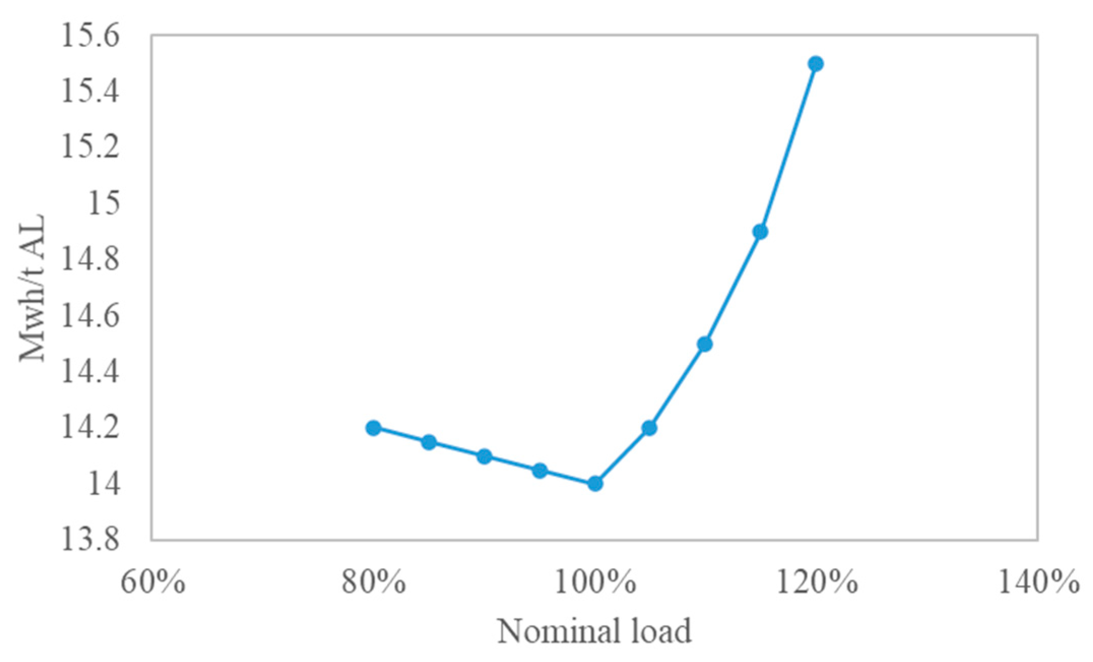
3.2.3. Exploring Operational Safety Boundaries

The operational safety of aluminum electrolyzers is determined by the temperature of the liquid aluminum. If the temperature of the electrolytic cell is too low, the electrolyte inside the cell will solidify on the sides and bottom, whereas the cryolite melt will freeze towards the carbon blocks, which will significantly reduce the thermal stability. Conversely, if the temperature goes too high, the cryolite melt could melt the cell walls, corrode the electrolytic cell, and thus shorten the service life of the electrolytic cell. Therefore, the safety operational limits of aluminum electrolyzers should be

$$\underset{¯}{T_e}\le T_e\le \overline{T_e}$$

(44)

where $T_e$ is the electrolyzer temperature, $\underset{¯}{T_e}$ and $\overline{T_e}$ are the lower and upper limits of the electrolyzer temperature, respectively.

Although it is possible to shut down the electrolyzer for a couple of hours, it is less likely that practical electrolytic aluminum plants to follow this request. Therefore, in this paper, shutting down the plant is not considered.

In practice, thermal parameters within aluminum electrolyzers may vary from case to case. It is risky to maintain the plant at its temperature boundary, as the thermal balance would become fragile and any disturbance would cause irreversible damage. Therefore, it would be more practical to determine a lower/upper production rate and a maximum load shifting period beyond the rate production. As a result, the operational strategy and principle of an electrolytic aluminum plant can be determined as

Table 2. Electrolytic aluminum load production stage.

Current	State	Production
[σ3Idc0, σ4Idc0)	Overload production	[Yas,min, Yas,r1)
[σ2Idc0, σ3Idc0)	Rate production	[Yas,r1, Yas,r2)
[σ1Idc0, σ2Idc0)	Reduced production	[Yas,r2, Yas,max]

and

Table 3. Electrolytic aluminum load production boundary.

State	Maximum-on Period	Minimum-off Period
Overload production	UThigh	DThigh
Rate production	/	/
Reduced production	UTlow	DTlow

.

Table 2 illustrates the maximum and minimum production limits for each state, while Table 3 presents that the maximum consecutive period of each state can be operated, and the minimum period of each state should be switch out before it is switch in again. To be more specific, when the plant decreases its operating current and production rate, its temperature will consistently decrease. Therefore, a maximum-on time should be determined to avoid the temperature exceeding the lower limit. On the contrary, when the plant switches to rate or overload production, it cannot switch back to the reduced production state before the temperature reaches the rate operating temperature.

Under this setup, the operational safety of the aluminum is assured to the greatest extent while maintaining adequate flexibility at the same time.

It is assumed that the rate production only allows the production rate to vary in a small range (95–105%), and the maximum and minimum production is at 80% and 120% of the rate production. The safety operational boundaries (maximum-on and minimum-off period) could be determined by performing the thermal dynamic model with (42) and (43) under the worst-case scenario.

To be more specific, Equations (42) and (43) can be solved in a finite difference scheme as

$${\displaystyle \frac{\partial T_e}{\partial t}}={\displaystyle \frac{T_{e,t+1}-T_{e,t}}{\Delta t}}$$

(45)

$${\displaystyle \frac{\partial T_s}{\partial t}}={\displaystyle \frac{T_{s,t+1}-T_{s,t}}{\Delta t}}$$

(46)

$$T_e={\displaystyle \frac{T_{e,t+1}+T_{e,t}}{2}}$$

(47)

$$T_s={\displaystyle \frac{T_{s,t+1}+T_{s,t}}{2}}$$

(48)

Referring to a typical electrolytic aluminum plant in Xinjiang Province, China, the rate voltage and current of the aluminum electrolytic cell is 4 V and 400 kA and the thermal parameters are as shown in

Table 4. Aluminum electrolyzer size parameters.

Component	Density/kg/m3	Volume/m3	Specific Heat Capacity /J/kg/°C
Electrolyte	2100	4	1600
Liquid aluminum	2700	9	880
Carbon blocks	2600	9	900

and

Table 5. Aluminum electrolyzer heat transfer parameters.

Component	Heat Transfer Coefficient/W/m2/°C	Heat Transfer Area/m2
Electrolyte–side shell	300	4
Liquid aluminum–side shell	200	4
Electrolyte–carbon blocks	5	3.6
Carbon blocks–air	5	60

, whereas the electrolyte temperature limits are 940–960 °C. The simulation results are shown below.

The simulation starts with a steady-state operation at the beginning, while the production rate shifting (i.e., from 100% to 80%/120% and from 80%/120% to 100%) occurs at the 2nd hour. Note that when the aluminum plant needs to increase or decrease its production rate, it will heat up raw materials to a higher or lower temperature (e.g., 930–980 °C for Al₂O₃ and 900–950 °C for carbon blocks) and hence accelerate the establishment of a new equilibrium. The resulting electrolyte temperature changes are shown in Figure 5 and Figure 6. It can be observed that the temperatures both exceed the limit after 4 h when the plant shifts from 100% to 80%/120%. The electrolyte temperatures could both change back to the rate temperature (950 °C) after 5 h when the plant shifts back to 100%.

3.2.4. Electrolytic Aluminum Plant Model Reformulation

After key operational safety parameters have been determined, the equivalent model of the electrolytic aluminum plant can be formulated as follows:

$$Y_{as,\min }{u}_{\mathrm{low},t}+Y_{as,\mathrm{r}1}{u}_{\mathrm{rate},t}+Y_{as,\mathrm{r}2}{u}_{\mathrm{high},t}\le Y_{as,t}\le Y_{as,\mathrm{r}1}{u}_{\mathrm{low},t}+Y_{as,\mathrm{r}2}{u}_{\mathrm{rate},t}+Y_{as,\max }{u}_{\mathrm{high},t}$$

(49)

$$\begin{array}{cc}{H}_{s,t}\ge H_{s,t-1}+u_{s,t}-(1-u_{s,t})\cdot \mathrm{M}& s=\left\{\mathrm{high},\mathrm{low}\right\}\end{array}$$

(50)

$$\begin{array}{cc}0\le H_{s,t}\le {\mathrm{UT}}_s& s=\left\{\mathrm{high},\mathrm{low}\right\}\end{array}$$

(51)

$$\begin{array}{cc}{y}_{s,t}-z_{s,t}=u_{s,t}-u_{s,t-1}& \forall s=\left\{\mathrm{high},\mathrm{low}\right\}\end{array}$$

(52)

$$\begin{array}{cc}{y}_{s,t}-z_{s,t}\le 1& \forall s=\left\{\mathrm{high},\mathrm{rate},\mathrm{low}\right\}\end{array}$$

(53)

$$\begin{array}{cc}{y}_{s,t},z_{s,t},u_{s,t}=\{0,1\}& \forall s=\left\{\mathrm{high},\mathrm{rate},\mathrm{low}\right\}\end{array}$$

(54)

$$\begin{array}{c}{\displaystyle \sum _{t=k}^{k+{\mathrm{DT}}_s-1}\left(1-u_{s,t}\right)\le {\mathrm{DT}}_s\cdot z_{s,k}}\\ \forall k=1\dots T-{\mathrm{DT}}_s+1,s=\left\{\mathrm{high},\mathrm{low}\right\}\end{array}$$

(55)

where s is the operational state index; u_s,t, y_s,t, and z_s,t are binary variables representing the operation sate of the electrolytic aluminum plant and actions of switch to and switch out of state s; H_s,t represents the consecutive period that the plant was in state s; UT_g and DT_g are maximum-on and minimum-off periods; and M is a very big positive number to guarantee that H_s,t can be reset once the plant switches out of state s.

According to (28)–(32), the production rate and power follows a nonlinear relationship:

$$Y_{as,t}=g(P_{AL,t})$$

(56)

As a result, Equation (56) can be linearized by (9)–(12) as well.

3.2.5. Additional Lower-Level Constraints

The lower-level optimization model aims to maximize the profit of the electrolytic aluminum plant:

$$\max C=C_{as}-C_{ass}-C_G-C_E-C_{CET,AL}$$

(57)

where C_ass is the cost of raw materials and additional depreciation and labor expenses caused by reduced/overload operation; C_as is the revenue of aluminum production; C_G is the cost of local thermal power generation; C_E is the cost of electricity purchased from the upper-level grid; and C_CET,AL represents the carbon trading cost.

The above cost component can be further represented as

$$C_{as}={\displaystyle \sum _t{\rho }_{AL}{Y}_{as,t}}$$

(58)

$$C_{ass}={\displaystyle \sum _{t,s}{\rho }_{r,s}\cdot u_{s,t}}$$

(59)

$$C_e={\lambda }_w{E}_w+{\lambda }_{pv}{E}_{pv}+{\lambda }_{G,\mathrm{buy}}{E}_{G,\mathrm{buy}}$$

(60)

where ρ_AL and ρ_r,s are the aluminum selling price and non-electricity production cost of operational state s; E_w, E_pv, and E_G,buy represent the amount of wind, solar, and thermal plant generation power purchased from the upper grid; and λ_w, λ_pv, and λ_G,buy represent the price of wind, solar, and thermal plant power from the upper grid.

Note that in practice, the electrolytic aluminum plant would have a self-owned power plant, which is usually a thermal power plant, whose generation cost C_G and constrains follow (5) and (16)–(25). Note that its cost constraint should also be linearized by (9)–(12).

In addition, the power balance at the plant level should be modeled:

$$P_{\mathrm{AL}}=E_w+E_{pv}+E_{G,\mathrm{buy}}+E_G$$

(61)

3.2.6. Tiered Carbon Trading Mechanism

Compared to the traditional carbon trading mechanism, to constrain carbon emissions, a tiered calculation of carbon trading costs based more strictly on segmented carbon emissions is adopted, and a price compensation coefficient is introduced.

The carbon trading cost of the electrolytic aluminum plant can be modeled as

$$C_{e,AL}={\gamma }_{AL}(E_{G,\mathrm{buy}}+E_G)$$

(62)

$$C_{q,AL}={\gamma }_{\mathrm{q},AL}{P}_{AL}$$

(63)

$$E_{AL}^{"}=C_{e,AL}-C_{q,AL}$$

(64)

where γ_AL represents the carbon emission coefficient per unit of thermal power for the electrolytic aluminum plant; γ_q,AL represents the allocation coefficient of the carbon emission quota; C_e,AL represents the actual carbon emissions of the electrolytic aluminum plant; C_q,AL represents the carbon quota of the enterprise; C_CET,AL represents the carbon trading cost for the electrolytic aluminum plant; and E″ represents the carbon emission trading volume for the electrolytic aluminum plant.

The tiered carbon mechanism formulates stricter rules for enterprises that exceed the carbon emission limit. The more the excess, the heavier the carbon penalty, which follows

$$C_{CET,AL}=\left\{\begin{array}{ll}\begin{array}{l}\mathsf{\lambda }(1+2\beta )\left(E^{″}+c\right)+\mathsf{\lambda }(1+\beta )c\\ \mathsf{\lambda }(1+\beta )E^{″}\\ \mathsf{\lambda }{E}^{″}\end{array}\hfill & \begin{array}{l}-2c<E^{″}\le c\\ -c<E^{″}\le 0\\ 0<E^{″}\le c\end{array}\hfill \\ \mathsf{\lambda }(1+\beta )\left(E^{″}-c\right)+\mathsf{\lambda }c\hfill & c<E^{″}\le 2c\hfill \\ \mathsf{\lambda }(1+2\beta )\left(E^{″}-2c\right)+\mathsf{\lambda }(2+\beta )c\hfill & 2c<E^{″}\le 3c\hfill \\ \mathsf{\lambda }(1+3\beta )\left(E^{″}-3c\right)+\mathsf{\lambda }(3+3\beta )c\hfill & 3c<E^{″}\le 4c\hfill \\ \mathsf{\lambda }(1+4\beta )\left(E^{″}-4c\right)+\mathsf{\lambda }(4+6\beta )c\hfill & E^{″}\ge 4c\hfill \end{array}\right.$$

(65)

where λ represents the base price for carbon trading, c represents the length of the carbon emission range, and β represents the price growth rate.

The piecewise-defined Equation (65) can be reformulated in a linear form as

$${\displaystyle \sum _k{E}_{\min ,k}^{″}{S}_k}\le E^{″}\le {\displaystyle \sum _k{E}_{\max ,k}^{″}{S}_k}$$

(66)

$${\displaystyle \sum _k{S}_k}=1$$

(67)

$$S_k\in \{0,1\}$$

(68)

$$C_{CET,AL}\ge {\mathsf{\omega }}_k^1{E}^{″}+{\mathsf{\omega }}_k^2-(1-S_k)\cdot \mathrm{M}$$

(69)

where S_k is a binary variable of the emission tier and ${\mathsf{\omega }}_k^1$ and ${\mathsf{\omega }}_k^2$ are coefficients of carbon prices in each segment in (65).

4. Case Studies

The case studies undertaken here are based on an electrolytic aluminum plant in Xinjiang Province, China. The upper-level main grid contains four thermal generation units, a wind farm, and a photovoltaic power generation station. The lower-level system includes an electrolytic aluminum plant with a total load power of 700 MW and a production rate of 50 kg aluminum/h (in rate operation), as well as a 330 MW self-owned thermal power plant. Detailed parameters regarding thermal generation units are shown in

Table 6. Thermal generation unit parameters.

Generators		Pmax	Pmin	a	b	c
Upper Level	CG1	370	111	2.54 × 10−2	131.5	5904
	CG2	270	81	2.09 × 10−2	123.1	4596
	CG3	160	48	4.89 × 10−2	155.5	2824
	CG4	100	30	6.20 × 10−2	162.3	2500
Lower Level	CGEAL	330	99	2.24 × 10−2	128.5	5310

, whereas the wind and solar power generation and upper-level electric load curves are shown in Figure 7.

The electrolytic aluminum plant power load–production curve is shown in Figure 8. Its operational safety parameters are summarized in

Table 7. Electrolytic aluminum plant operational safety boundaries.

State	Max-on Period	Min-off Period	Production Range
Overload production	4 h	5 h	105–120%
Rate production	/	/	95–105%
Reduced production	4 h	5 h	80–95%

, determined by the method presented in Section 3.2.3.

The upper-level green certificate purchase and selling price are CNY 50 and 35 per unit, respectively. The lower-level carbon emission quota coefficient is 40%, whereas the carbon base price, length of emission range, and carbon price growth rate are set to be 80 CNY/ton, 1000 ton, and 30%, referring to the current carbon market in China. The resulting emission–cost diagram is shown in Figure 9.

To analyze the effectiveness of the proposed two-level optimization framework on decarbonizing the energy system, three cases are presented:

Case 1: The electrolytic aluminum plant is operated at a constant production rate, with no carbon policy introduced.

Case 2: The electrolytic aluminum plant is operated at a varying production rate considering the operational safety limits, with no carbon policy introduced.

Case 3: The electrolytic aluminum plant is operated at a varying production rate, with green certificate trading and tiered carbon emission trading mechanisms introduced.

4.1. Dispatching Results

The resulting generation mix and aluminum production rate of Case 1 are shown in Figure 10 and Figure 11. It can be observed that the electrolytic aluminum load remains constant, whereas the upper-level system relies solely on thermal generator operations to integrate renewable power where severe wind and solar curtailment occurs.

The dispatching results of Case 2 are shown in Figure 12 and Figure 13. After considering the operational characteristics of the electrolytic aluminum load, it can be observed that the wind power generation at the lower level has significantly increased at the beginning and end of the day to match with the electrolytic aluminum load. However, the thermal power generation has decreased at the middle of the day to follow the load shedding provided by the electrolytic aluminum load. This is because at the beginning and end of the day, the aluminum plant uses surplus wind power to produce the aluminum at a cheaper electricity price. As long as the production cost is lower than the aluminum selling price, the plant would use whichever power it can obtain to increase its production. At the middle of the day when the renewable generation is smaller, the average electricity price that can be used to produce aluminum is higher and becomes uneconomic, and hence the plant would lower its production rate during this period.

The dispatching results of Case 3 are shown in Figure 14 and Figure 15, where green certificate trading and tiered carbon emission trading mechanisms are both introduced. In this case, the two-level coordinated scheduling of electricity, aluminum, and carbon is achieved. The electrolytic aluminum plant would lower its production and operate more on the reduced production state to reduce the emissions.

Note that in all three cases, the upper-level PV generation is insufficient and cannot be used by the lower-level electrolytic aluminum plant.

4.2. Cost–Benefit Analysis

The upper-level operational cost, lower-level plant revenue, and the emissions for the three cases are shown in

Table 8. Result summary.

Case	Upper-Level Cost (×103 CNY)	Plant Revenue (×103 CNY)	Emission (tons/day)
Case 1	1860	3855	10,198
Case 2	1884	4142	9495
Case 3	1554	3559	7969

, whereas the wind power utilization profiles are shown in Figure 16. Compared with Case 1, Case 2 shows how flexible operation of the electrolytic aluminum plant can affect the cost–benefit of the system and the integration level of the renewables. As the aluminum production increases, the plant revenue increases by 7.4%. The emission level decreases by 6.9% when carbon policy is not yet introduced. In Case 3, the upper-level operational cost is significantly decreased by 16.5%, as the system produces large amount of renewable power and obtains additional revenue from green certificate trading. The system emission decreases by 21.9% as a result of carbon trading, accounting for 2229 tons compared with Case 1.

The renewable integration level of the three cases is shown in Figure 16. In Case 1, the number of time periods with renewable curtailment is 10, with a maximum curtailed power of 130 MW. The total amount of wind and solar curtailment is 629.99 MWh, and the curtailment rate is 4.89%. In Case 2, the maximum curtailed wind and solar power is 59 MW, with a total curtailment of 117.5 MWh and a curtailment rate of 0.91%. In Case 3, the maximum curtailed wind and solar power is only 21 MW, with a total curtailment of 50 MWh and a curtailment rate of 0.39%.

From the above analysis, it can be concluded that the proposed two-level model considering electricity–aluminum–carbon coordinated scheduling increases the economic efficiency of the system, reduces carbon emissions, and lowers the wind and solar curtailment rate. This validates that the proposed scheduling strategy improves the system’s economic performance while bringing environmental benefits.

4.3. Sensitivity Analysis

The carbon prices in China remains low (80 CNY/ton), whereas in the carbon prices in the EU have reached around 500 CNY/ton (60–70 EUR/ton) [26]. Considering China’s carbon neutrality goals, the future carbon policy will possibly become stricter. Therefore, this subsection analyzes the influence of key parameters regarding carbon prices.

The resulting aluminum production, carbon emission, and plant revenue under different carbon price parameters are shown in

Table 9. Carbon price sensitivity analysis.

Parameters (λ, β)	Production (ton AL)	Plant Revenue (×103 CNY)	Plant Emission (tons/day)
(80, 30%)	1.173	3559	7969
(80, 50%)	1.168	3495	7906
(200, 50%)	1.124	2884	7418
(500, 50%)	1.095	1547	7089

. It can be observed that the plant revenue would reduce with the increase in the base carbon price and carbon price growth rate, causing the plant to reduce production and the usage of thermal power.

5. Conclusions

This paper proposes a two-level low-carbon economic scheduling framework for the coordinate optimization of an electricity–aluminum–carbon energy system that facilities renewable integration and carbon reduction by green certificate and tiered carbon trading mechanisms by the flexible operation of an electrolytic aluminum plant. Specifically, this work presents a safety-constrained electrolytic aluminum plant model, considering its multiple operational states and practical limitations of state changing, with key parameters obtained by performing a thermal dynamic simulation of the electrolytic aluminum plant under critical scenarios.

The case studies presented show that, compared with the traditional operation mode, the flexible operation of an electrolytic aluminum plant can increase the renewable integration rate by 4.0% and reduce emissions by 6.9%. By adopting the carbon trading mechanisms with the current carbon price in China, the system can significantly reduce the emission by 21.9% and improve its overall economic efficiency by 16.5%. A sensitivity analysis was conducted with respect to different carbon trading parameters, showing that a maximum carbon reduction of 30.5% can be achieved with the current EU carbon price policies.

Future research will focus on the real-time scheduling of electrolytic aluminum plants and explore the impact of electrolytic aluminum loads on power grid balances and frequency regulations.

References

1. National Development and Reform Commission of China. Guiding Opinions on Vigorously Implementing the Renewable Energy Substitution Action; National Development and Reform Commission of China: Beijing, China, 2024.
2. Guiding Opinions on Energy Work in 2024. 2024. Available online: https://www.nea.gov.cn (accessed on 28 February 2025).
3. Sharma, R.; Sinha, A.; Kautish, P.; Paul, S.; Dey, T.; Saha, P.; Dey, S.; Sen, R. Review on the development scenario of renewable energy in different country. In Proceedings of the 2021 Innovations in Energy Management and Renewable Resources, Kolkata, India, 30 March 2021. [Google Scholar]
4. Zhang, J.; Li, L.; Yan, T.; Yu, J.; He, C.; Liao, S. A collaborative control method for high-proportion renewable energy and flexible loads. In Proceedings of the 2024 4th International Conference on Energy, Power and Electrical Engineering (EPEE), Wuhan, China, 17 February 2025. [Google Scholar]
5. Yang, Z.; Ren, Z.; Li, H.; Sun, Z.; Feng, J.; Xia, W. A multi-stage stochastic dispatching method for electricity-hydrogen integrated energy systems driven by model and data. Appl. Energy 2024, 371, 123668. [Google Scholar] [CrossRef]
6. Yang, N.; Xu, G.; Fei, Z.; Li, Z.; Du, L.; Guerrero, J.M.; Huang, Y.; Yan, J.; Xing, C.; Li, Z. Two-Stage Coordinated Robust Planning of Multi-Energy Ship Microgrids Considering Thermal Inertia and Ship Navigation. IEEE Trans. Smart Grid 2025, 16, 1100–1111. [Google Scholar] [CrossRef]
7. Liu, J.; Wang, K.; Su, Z.; Feng, Y.; Wang, C.; Ai, X. Source-load Coordinated Optimal Scheduling in Stochastic Unit Commitment Considered Electrolytic Aluminum Load and Wind Power Uncertainty. In Proceedings of the 2022 IEEE 5th International Electrical and Energy Conference (CIEEC), Nangjing, China, 11 August 2022. [Google Scholar]
8. Li, L.; Chen, Y.; Zhang, J.; Pi, S.; He, C.; Liao, S. High-capacity Multi-level Emergency Load Shedding Technology for Electrolytic Aluminum Load. In Proceedings of the 2023 8th International Conference on Power and Renewable Energy (ICPRE), Shanghai, China, 22–25 September 2023. [Google Scholar]
9. Li, L.; Chen, Y.; Sun, P.; He, C.; Pi, S.; Liao, S. Real-Time Regulation Boundary Solution Method for Electrolytic Aluminum Industrial Park. In Proceedings of the 2024 3rd International Conference on Power Systems and Electrical Technology (PSET), Tokyo, Japan, 30 December 2024. [Google Scholar]
10. Adibi, T.; Sojoudi, A.; Saha, S.C. Modeling of thermal performance of a commercial alkaline electrolyzer supplied with various electrical currents. Int. J. Thermofluids 2022, 13, 100126. [Google Scholar] [CrossRef]
11. Paulus, M.; Borggrefe, F. The potential of demand-side management in energy-intensive industries for electricity markets in Germany. Appl. Energy 2011, 88, 432–441. [Google Scholar]
12. Zeng, K.; Wang, H.; Liu, J.; Dong, C.; Lan, X.; Wang, C.; Le, L.; Ai, X. A bi-level programming guiding electrolytic aluminum load for demand response. In Proceedings of the 2020 IEEE/IAS Industrial and Commercial Power System Asia (I&CPS Asia), Weihai, China, 13–15 July 2020. [Google Scholar]
13. Zhou, B.; Li, J.; Liu, Q.; Li, G.; Gu, P.; Ning, L.; Wang, Z. Optimal operation of energy-intensive load considering electricity carbon market. Heliyon 2024, 10, e34796. [Google Scholar] [PubMed]
14. Gong, F.; Ren, K.; Zhang, A.; Chen, S.; Feng, J.; Zhang, K.; Li, D. Review of electrolytic aluminum load participating in demand response to absorb new energy potential and methods. In Proceedings of the 2021 IEEE 2nd International Conference on Big Data, Artificial Intelligence and Internet of Things Engineering (ICBAIE), Nanchang, China, 26–28 March 2021. [Google Scholar]
15. Ding, X.; Liao, S.; Xu, J.; Sun, Y. A Source-Load Coordinated Control Strategy in an Industrial Aluminum Production Mircrogrid for Smoothing Wind Power Fluctuations. In Proceedings of the 2023 IEEE/IAS Industrial and Commercial Power System Asia (I&CPS Asia), Chongqing, China, 7–9 July 2023. [Google Scholar]
16. Li, L.F.; Chen, Y.; Zhu, X.; Yu, Q.; Jiang, X.; Liao, S. Electrolytic Aluminum Load Participating in Power Grid Frequency Modulation Method Based on Active Adjustable Capacity Coordination. In Proceedings of the 2021 3rd Asia Energy and Electrical Engineering Symposium (AEEES), Chengdu, China, 26–29 March 2021. [Google Scholar]
17. Chen, S.; Gong, F.; Sun, T.; Yuan, J.; Yang, S.; Liu, Z. Research on the method of electrolytic aluminum load participating in the frequency control of power grid. In Proceedings of the 2021 IEEE 2nd International Conference on Big Data, Artificial Intelligence and Internet of Things Engineering (ICBAIE), Nanchang, China, 26–28 March 2021. [Google Scholar]
18. Liu, J.; Zeng, K.; Wang, C.; Le, L.; Zhang, M.; Ai, X. Unit commitment considering electrolytic aluminum load for ancillary service. In Proceedings of the 2019 4th International Conference on Intelligent Green Building and Smart Grid (IGBSG), Hubei, China, 6–9 September 2019. [Google Scholar]
19. Wang, Y.; Fu, B.; Ding, K.; Sun, Y. Day-ahead Economic Dispatch of Power Systems Considering the Demand Response of Electrolytic Aluminum Loads. In Proceedings of the 2024 IEEE 2nd International Conference on Power Science and Technology (ICPST), Dali, China, 9–11 May 2024. [Google Scholar]
20. Zheng, W.; Yu, P.; Xu, Z.; Fan, T.; Liu, H.; Yu, M.; Zhang, J.; Li, J. Day-ahead Intra-day Economic Dispatch Methodology Accounting for the Participation of Electrolytic Aluminum Loads and Energy Storage in Power System Peaking. In Proceedings of the 2024 IEEE 2nd International Conference on Power Science and Technology (ICPST), Dali, China, 9–11 May 2024. [Google Scholar]
21. Li, X.; Deng, J.; Liu, J. Energy–carbon–green certificates management strategy for integrated energy system using carbon–green certificates double-direction interaction. Renew. Energy 2025, 238, 121937. [Google Scholar]
22. Yang, Y.; Li, S.; Zhang, Z.; Zhang, N.; Wang, S.; Wu, X.; Yan, H. The low-carbon economic scheduling method for regional integrated energy systems considering the joint integration of electric vehicles and concentrated solar power plants for wind power consumption. Wind Eng. 2025, 309524, 241302464. [Google Scholar]
23. Gao, C.; Lu, H.; Chen, M.; Chang, X.; Zheng, C. A low-carbon optimization of integrated energy system dispatch under multi-system coupling of electricity-heat-gas-hydrogen based on stepwise carbon trading. Int. J. Hydrogen Energy 2025, 97, 362–376. [Google Scholar]
24. Sun, H.; Sun, X.; Kou, L.; Zhang, B.; Zhu, X. Optimal scheduling of park-level integrated energy system considering ladder-type carbon trading mechanism and flexible loa. Energy Rep. 2023, 9, 3417–3430. [Google Scholar]
25. National Development and Reform Commission of China. Special Action Plan for Energy Conservation and Carbon Emission Reduction in the Electrolytic Aluminum Industry; National Development and Reform Commission of China: Beijing, China, 2024.
26. EU Carbon Permits. Available online: https://tradingeconomics.com/commodity/carbon (accessed on 26 February 2025).
Figure 1. Solution process of the electric–aluminum–carbon collaborative two-level optimization model.
Energies 18 01645 g001
Figure 2. Renewable energy output curves for each scenario before reduction.(Diffirent colors refer to diffirent original wind/solar data).
Energies 18 01645 g002
Figure 3. Renewable energy output curves for each scenario after reduction. (Diffirent colors refer to diffirent scenarios).
Energies 18 01645 g003
Figure 4. Thermal balance diagram of the aluminum electrolytic cell.
Energies 18 01645 g004
Figure 5. Electrolyte temperature change when production reduced/overloaded.
Energies 18 01645 g005
Figure 6. Electrolyte temperature change when production shifts back to rate.
Energies 18 01645 g006
Figure 7. Upper-level input profiles.
Energies 18 01645 g007
Figure 8. Operational characteristics of the electrolytic aluminum plant.
Energies 18 01645 g008
Figure 9. Lower−level emission−carbon cost diagram.
Energies 18 01645 g009
Figure 10. The upper-level scheduling results for Case 1.
Energies 18 01645 g010
Figure 11. The lower-level scheduling results for Case 1.
Energies 18 01645 g011
Figure 12. The upper-level scheduling results for Case 2.
Energies 18 01645 g012
Figure 13. The lower-level scheduling results for Case 2.
Energies 18 01645 g013
Figure 14. The upper-level scheduling results for Case 3.
Energies 18 01645 g014
Figure 15. The lower-level scheduling results for Case 3.
Energies 18 01645 g015
Figure 16. Wind power integration levels.
Energies 18 01645 g016