Convex Optimization and PV Inverter Control Strategy-Based Research on Active Distribution Networks

Abstract

Optimizing the operation of active distribution networks (ADNs) has become more challenging because of the uncertainty created by the high penetration level of distributed photovoltaic (PV). From the convex optimization perspective, this paper proposes a two-layer optimization model to simplify the solution of the ADN optimal operation problem. Firstly, to pick out the ADN “key” nodes, a “key” nodes selection approach that used improved K-means clustering algorithm and two indexes (integrated voltage sensitivity and reactive power-balance degree) is introduced. Then, a two-layer ADN optimization model is built using various time scales. The upper layer is a long-time-scale model with on-load tap-changer transformer (OLTC) and capacitor bank (CB), and the lower layer is a short-time-scale optimization model with PV inverters and distributed energy storages (ESs). To take into account the PV users’ interests, maximizing PV active power output is added to the objective. Afterwards, under the application of the second-order cone programming (SOCP) power-flow model, a linearization method of OLTC model and its tap change frequency constraints are proposed. The linear OLTC model, together with the linear models of the other equipment, constructs a mixed-integer second-order cone convex optimization (MISOCP) model. Finally, the effectiveness of the proposed method is verified by solving the IEEE33 node system using the CPLEX solver.

1. Introduction

The green and low-carbon transition of energy is the key to realize the “dual-carbon” goals. The high penetration level of distributed generators (DG) has led to problems such as node voltage exceeding and power-flow reversal, and has posed a huge challenge to power system’s stable and economic operation [1,2,3]. Therefore, building new power systems is inevitable [4]. As an important part of the new power system, the distribution network is connected to numerous power electronic devices and has a higher operational complexity. In order to fully leverage the energy and the distribution network’s advantages to cope with the above problems, the proposal of an ADN voltage-control strategy with both flexibility and reliability is urgently needed.

PV inverters have the ability of reactive power regulation, which can realize continuous voltage/var control within a certain range. The PV inverters have four kinds of control strategies: maximum active power output control, reactive power control (RPC), active power curtailment (APC), and optimal inverter dispatch (OID) [5,6,7]. The flexible switching of different control strategies can realize the flexible active and reactive power output regulation. In current practical applications, most of the PV inverters use a single control strategy [8], i.e., maximum active power output control, which limits the flexibility of PV inverters’ regulation. In addition, at some specific times, the PV active power output is too high to be used up, which may result in the wasting of resources such as abandoned light. Therefore, the PV inverters control strategy that can fully utilize the advantages of multiple control strategies and can take into account the users’ interests is needed.

There are three types of methods for solving the ADN voltage/var control problem: artificial intelligence algorithms (AI), data-driven methods, and mathematical methods. However, AI algorithms cannot guarantee the convergence to the global optimum; data-driven algorithms require a large amount of data; mathematical methods, which use solvers to solve problems, are more reliable but struggle to directly solve complex nonlinear problems [9]. The ADN voltage/var control problem is essentially a high-dimensional and high-complex mixed-integer nonlinear programming (MINLP) problem which is difficult to solve and needs to be linearized first. By using the second-order cone relaxation, semidefinite relaxation and linear approximation, Refs. [10,11,12,13] convexified the non-convex power-flow model and proposed the SOCP power-flow model, the semidefinite programming (SDP) power-flow model, and the linear approximation (LA) power-flow model, respectively. SDP model is more accurate but takes a long time to solve; the LA model is simple and takes less time but has large errors; and the SOCP model is the most widely used one. Ref. [14] proposed a method to linearize the ADN OLTC model by using the big M method under the application of the SOCP power-flow model. The big M method is a linearization approach and has the extensive application in the linearization of nonlinear constraints. Its fundamental principle lies in leveraging an arbitrarily large positive number M to relax the original nonlinear constraints into linear ones [15,16]. Ref. [17] solved the optimization of electric stress distribution over the live electrode of an axisymmetric vacuum interrupter employed for 11 kV switching operations, which is a MINLP problem by using the big M method. Although the Ref. [14] can successfully linearize the OLTC model, it requires multiple variable substitutions which increase the linear model complexity and make the model hard to solve. Therefore, a simple linear OLTC model that can be applied under the SOCP power-flow model is necessary.

The injected power’s effect on ADN node voltages is different. To fully utilize the compensation devices, it is essential for device allocation to evaluate the power injection impact on node voltages and select high-impact “key” nodes. The typical indicators used for evaluation are reactive voltage sensitivity [18], edge weight [19], power transfer distribution factor (PTDF) [20], reactive power-balance degree [21], etc. Ref. [22] partitioned the power system based on a comprehensive electrical distance index. Ref. [23] partitioned the distribution networks by using the labeled numbers of the nodes on paths between every two adjacent controllable distributed generations (CDG) as the optimization variables. Power system partitioning usually uses clustering methods; the typical and simple ones are K-means clustering [24], K-means++ clustering, fuzzy clustering [25], etc. K-means clustering is simple in principle, fast in computation, and feasible in practice. However, for the traditional K-means clustering method, it is sensitive to the initial clustering centers and the selection of initial centers is random. Improper clustering centers can cause problems such as local optimality, slow convergence, and instability. Therefore, when applying the K-means clustering algorithm, the selection of suitable initial clustering centers is very important. In addition, the $R/X$ of the distribution network is relatively low [26,27,28], so it is necessary to consider both active and reactive power effects on the ADN node voltages.

In summary, the key contributions of this paper are as follows:

1.

Given the single control strategy of PV inverters that restricts reactive power regulation and flexibility, a comprehensive control strategy integrating multiple strategies is proposed. This aims to fully exploit the regulation capacity and account for users’ interests.

2.

Considering the complex and non-simplified OLTC models under the SOCP power-flow model, an OLTC model linearization approach using integers binary expansion and the big M method is proposed. Additionally, a linear model for OLTC tap change frequency constraints is put forward.

3.

Since current “key” nodes selection indicators in distribution networks mainly focus on reactive power effect while overlooking the active power effect, a comprehensive index encompassing active–reactive voltage sensitivity and reactive power-balance degree is proposed.

4.

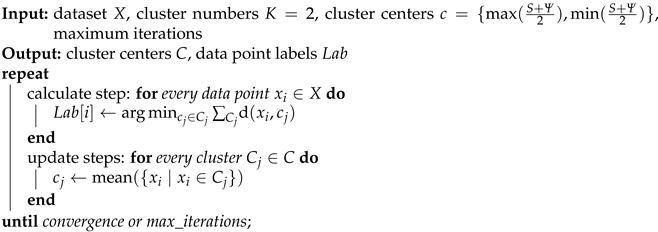
Due to the random selection of initial clustering centers in the traditional K-means algorithm, an improved K-means clustering algorithm with an enhanced selection method for initial clustering centers is proposed.

This research was based on the improved IEEE33 case system.

2. Key Nodes Selection

Active-reactive voltage sensitivity and reactive power-balance degree constituted the comprehensive evaluation index together. The comprehensive evaluation index and the improved k-means clustering method were used to classify the nodes into “key” ones and “normal” ones.

2.1. Active–Reactive Voltage Sensitivity

The active–reactive voltage sensitivity was obtained by calculating the voltage sensitivity matrix, and the process is shown below.

Let there be a system with n nodes, where there is 1 balanced node, m PV nodes, and the others are PQ nodes. In polar coordinate, the power equations for each node of the system are shown in Equation (1) [29].

$$\left\{\begin{array}{c}△P_i=P_{Gi}-P_{Li}-U_i\sum _{j\in i}{U}_j(G_{ij}cos{\theta }_{ij}+B_{ij}sin{\theta }_{ij})=0,(i=1, 2, \dots , n-1)\hfill \\ △Q_i=Q_{Gi}-Q_{Li}-U_i\sum _{j\in i}{U}_j(G_{ij}sin{\theta }_{ij}-B_{ij}cos{\theta }_{ij})=0,(i=1, 2, \dots , m)\hfill \end{array}\right.$$

(1)

where $P_{Gi}-P_{Li}$ is the active power injection of node i; $Q_{Gi}-Q_{Li}$ is the reactive power injection of node i.

Then, based on the Newton–Raphson method, Equation (2) can be derived as follows.

$$\left[\begin{array}{c}\Delta P\\ \Delta Q\end{array}\right]=J\left[\begin{array}{c}\Delta \theta \\ \Delta V\end{array}\right]=\left[\begin{array}{cc}{\displaystyle \frac{\partial P}{\partial Q}}& {\displaystyle \frac{\partial P}{\partial V}}\\ {\displaystyle \frac{\partial Q}{\partial \theta }}& {\displaystyle \frac{\partial Q}{\partial V}}\end{array}\right]\left[\begin{array}{c}\Delta \theta \\ \Delta V\end{array}\right]$$

(2)

where J is the Jacobi matrix.

The voltage sensitivity matrix can be obtained by inverting J as shown in Equation (3) [30,31,32].

$$\left[\begin{array}{c}\Delta \theta \\ \Delta V\end{array}\right]=J^{-1}\left[\begin{array}{c}\Delta P\\ \Delta Q\end{array}\right]=\left[\begin{array}{cc}{\displaystyle \frac{\partial \theta }{\partial P}}& {\displaystyle \frac{\partial \theta }{\partial Q}}\\ {\displaystyle \frac{\partial V}{\partial P}}& {\displaystyle \frac{\partial V}{\partial Q}}\end{array}\right]\left[\begin{array}{c}\Delta P\\ \Delta Q\end{array}\right]$$

(3)

let $A_{ij}=\partial V_i/\partial P_j$ and $B=\partial V/\partial Q$, A and B are the active and reactive voltage sensitivity matrices, respectively, where $A_{ij}$ denotes the effect of the node j active change on the node i voltage, i.e., the node i sensitivity to the node j active change. The diagonal elements of matrix $A_{ij}$ describe the voltage sensitivity of the node’s active change to itself; the non-diagonal elements of matrix $A_{ij}$ describe the voltage sensitivity of the node’s active change to others. $A_{ij}>0$ indicates that increasing the j node active injection can improve the i node voltage stability; $A_{ij}<0$ indicates that increasing the j node active injection will worsen the i node voltage stability. The reactive voltage sensitivity is the same.

Take the absolute value sum of each node’s active voltage sensitivity and reactive voltage sensitivity, as shown in Equations (4) and (5).

$$S_i^P=\sum _{j\in N}\left|A_{ij}\right|$$

(4)

$$S_i^O=\sum _{j\in N}\left|B_{ij}\right|$$

(5)

where N is the set of all nodes.

The comprehensive i node voltage sensitivity can be obtained by normalizing and summing the active and reactive voltage sensitivities, respectively. As shown in Equation (6).

$$S_i={\mu }_1{\displaystyle \frac{S_i^P}{\overline{S^P}}}+{\mu }_2{\displaystyle \frac{S_i^Q}{\overline{S^Q}}}$$

(6)

where ${\mu }_1$ and ${\mu }_2$ are the weight factors, and both of them are taken as 0.5 [33]; $\overline{S^P}$ and $\overline{S^Q}$ are the maximum values of $S^P$ and $S^Q$.

2.2. Reactive Power-Balance Degree

The reactive power-balance degree was used to describe the level of the node’s reactive power compensation required. The bigger the degree, the higher level of node reactive power compensation required, as shown in Equation (7) [21].

$${\Psi }_i=\left\{\begin{array}{cc}0\hfill & ,Q_{i,needed}=0\hfill \\ \left|{\displaystyle \frac{\frac{Q_{i,needed}}{Q_{i,needed}+Q_{i,supplied}}}{\overline{\frac{Q_{i,needed}}{Q_{i,needed}+Q_{i,supplied}}}}}\right|\hfill & ,Q_{i,needed}\ne 0\hfill \end{array}\right.$$

(7)

where $Q_{i,needed}$ is the additional reactive power at node i to qualify the node voltage (0.95 p.u.); $Q_{i,supplied}$ is the reactive power supplied to node i in the actual power flow. The formulation of $Q_{i,needed}$ is shown in Equation (2).

$$\left\{\begin{array}{cc}{U}_i\ge 0.95 \mathrm{p}.\mathrm{u}.\hfill & ,Q_{i,needed}=0\hfill \\ U_i<0.95 \mathrm{p}.\mathrm{u}.\hfill & ,Q_{j,needed}={\displaystyle \frac{0.95 \Delta V_j}{X_{ij}}}\hfill \end{array}\right.$$

(8)

where $\Delta V_j=0.95-V_j$.

2.3. Node Classification Method Based on Improved K-Means Clustering

The K-means clustering algorithm is one of the most widely used clustering algorithms and also can be used to classify the “key” nodes. The algorithm is simple and useful, but the selection of its clustering number K and initial clustering center directly affects the clustering results [34].

The basic principle of the K-means algorithm is to divide the dataset $X=x_1, x_2, \dots , x_n$ ($x_i=(x_{i1}, x_{i2}, \dots , x_{id})$ is a d-dimensional vector) into K clusters according to the rule that the sum of squares of all points in the clusters to their clustering centers are the smallest. Each cluster corresponds to a clustering center, as shown in Equation (9).

$$min\sum _{i=1}^K\sum _{X\in C_i}{\parallel x-c_i\parallel }_2^2$$

(9)

where $X\in C_i$ denotes the sample in the ith cluster; $c_i$ denotes the ith cluster’s clustering center.

In this research, the ADN nodes need to be classified into “key” ones and “normal” ones by applying K-means clustering algorithm. Therefore, take $K=2$.

Since the initial clustering centers of the traditional K-means method are randomly selected, which may lead to slow convergence, the selection way of the initial centers is improved.

The nodes’ active–reactive voltage sensitivities and reactive power imbalance degrees are positively correlated, and it is hoped that the selected “key” nodes have large values of both indexes, so the two points with the largest and smallest indexes mean values were selected as the initial centers, as shown in Equation (10).

$$C=\{max\left({\displaystyle \frac{S+\Psi }{2}}\right),min\left({\displaystyle \frac{S+\Psi }{2}}\right)\}$$

(10)

The pseudo-code of the improved K-means clustering algorithm is shown in Algorithm 1.

Algorithm 1 Improved K-means clustering algorithm.

3. The Framework of ADN Optimization Operation Model

Let the set of all ADN nodes be N (node 1 is the balanced node), the set of the nodes with PV access be $N_{PV}$, the set of the nodes with ES access be $N_{ES}$, the set of the nodes with CB access be $N_{CB}$, the set of the nodes with OLTC access be $N_{OLTC}$, and the set of all lines be L.

3.1. Upper-Layer Optimization Model

In the upper-layer model, the time scale is one hour and the devices are OLTC and CBs.

3.1.1. Upper-Layer Model Constraints

1.

Power-flow constraints

Using the branch flow model shown in Figure 1, the branch flow equation shown in Equation (11) is listed according to Ohm’s law, the branch first-end power equation and the node power-balance equation.

$$\left\{\begin{array}{c}{S}_{ij}^t=V_i^t{I}_{ij}^{t*}\hfill \\ V_j^t=V_i^t-Z_{ij}{I}_{ij}^t\hfill \\ S_j^t=\sum _{k:j\to k}{S}_{jk}^t-\sum _{i:i\to j}(S_{ij}^t-Z_{ij}|I_{ij}^t{|}^2)\hfill \end{array}\right.$$

(11)

where $i,j\in N;(i,j),(j,k)\in L;t\in T=1, \dots , 24$; $S_{ij}$ and $I_{ij}$ are branch $(i,j)$’s transmission power and current; $S_j$ is the injection power of node i, its value is the difference between the power emitted by the generator and the load at node i, i.e., $S_i=S_i^g-S_i^l$.

2.

OLTC model

The low voltage side of the OLTC is connected to the balancing node. To simplify the solution of the optimization problem, only the low voltage side of the OLTC is considered. Let the OLTC be an ideal one and set the reference voltage $V_{ref}=1$. The OLTC model is shown in Equation (12).

$$\left\{\begin{array}{c}0\le T^t\le K\hfill \\ V_1^t=V_{ref}·k^t\hfill \\ k^t=1+(T^t-2)\Delta k\hfill \end{array}\right.,t\in T=1, \dots , 24$$

(12)

where $T^t$ is the OLTC tap at moment t, the integer variables; $\Delta k$ is the step size between adjacent taps, its value is 2.5%; K is the total number of taps, its value is 4.

3.

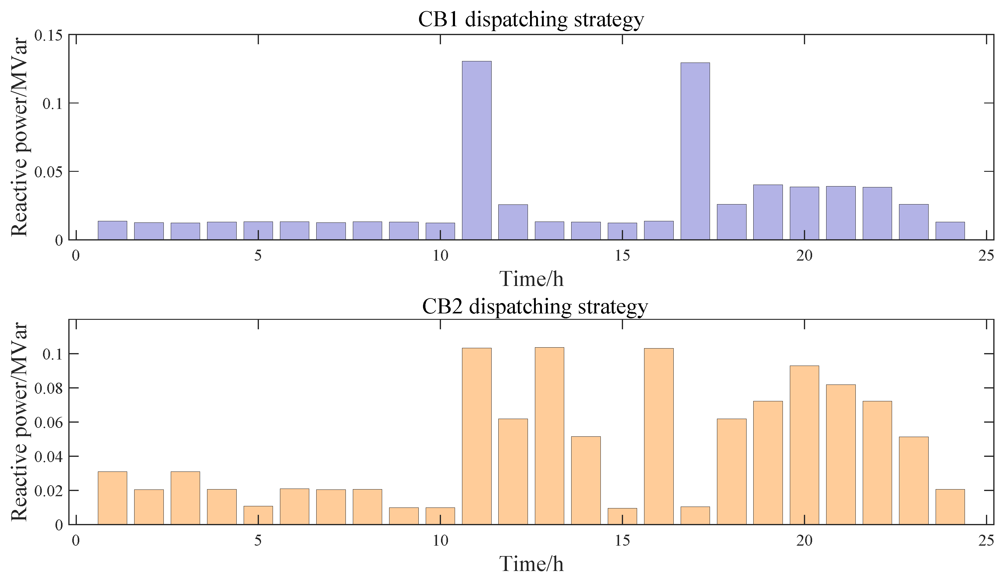
CB model

The CB model is shown in Equation (13).

$$\left\{\begin{array}{c}{q}_j^{c,t}=d_j^t{q}_j^{step}\hfill \\ 0\le d_j^t\le n_j^c\hfill \\ q_j^t=q_j^{c,t}-q_j^{L,t}\hfill \end{array}\right.,j\in N_{CB};t\in T=1, \dots , 24$$

(13)

where $q_j^{c,t}$ is the reactive power compensated by the CB at node j; $d_j$ is the number of CB banks to be switched, the integer variables; $q_j^{step}$ is the capacity of each CB bank; $n_j^c$ is the total number of CB banks connected at node j; $q_j^L$ is the reactive power consumed by the load at node j.

4.

Node voltage constraint

$$\underline{V_i}\le V_i^t\le \overline{V_i},t\in T=1, \dots , 24$$

(14)

where $V_i$ is the voltage of node i; $\underline{V_i}$ and $\overline{V_i}$ are the upper and lower limits of the node i voltage, respectively.

5.

Branch current constraint

$$0\le I_{ij}^t\le \overline{I_{ij}},t\in T=1, \dots , 24$$

(15)

where $I_{ij}^t$ is the maximum current of branch $(i,j)$.

3.1.2. Upper-Layer Model Objective Function

The objective function of the upper-layer is the active network loss. According to Ohm’s law, the active network loss is defined as shown in Equation (16).

$$min{F}_1=min\sum _{t\in T}\sum _{i\in N}{R}_{ij}{\left(I_{ij}^t\right)}^2,t\in T=1, \dots , 24$$

(16)

3.2. Lower-Layer Optimization Model

In the lower-layer model, the time scale is 30 min and the devices are PV inverters and ESs.

3.2.1. Lower-Layer Model Constraints

1.

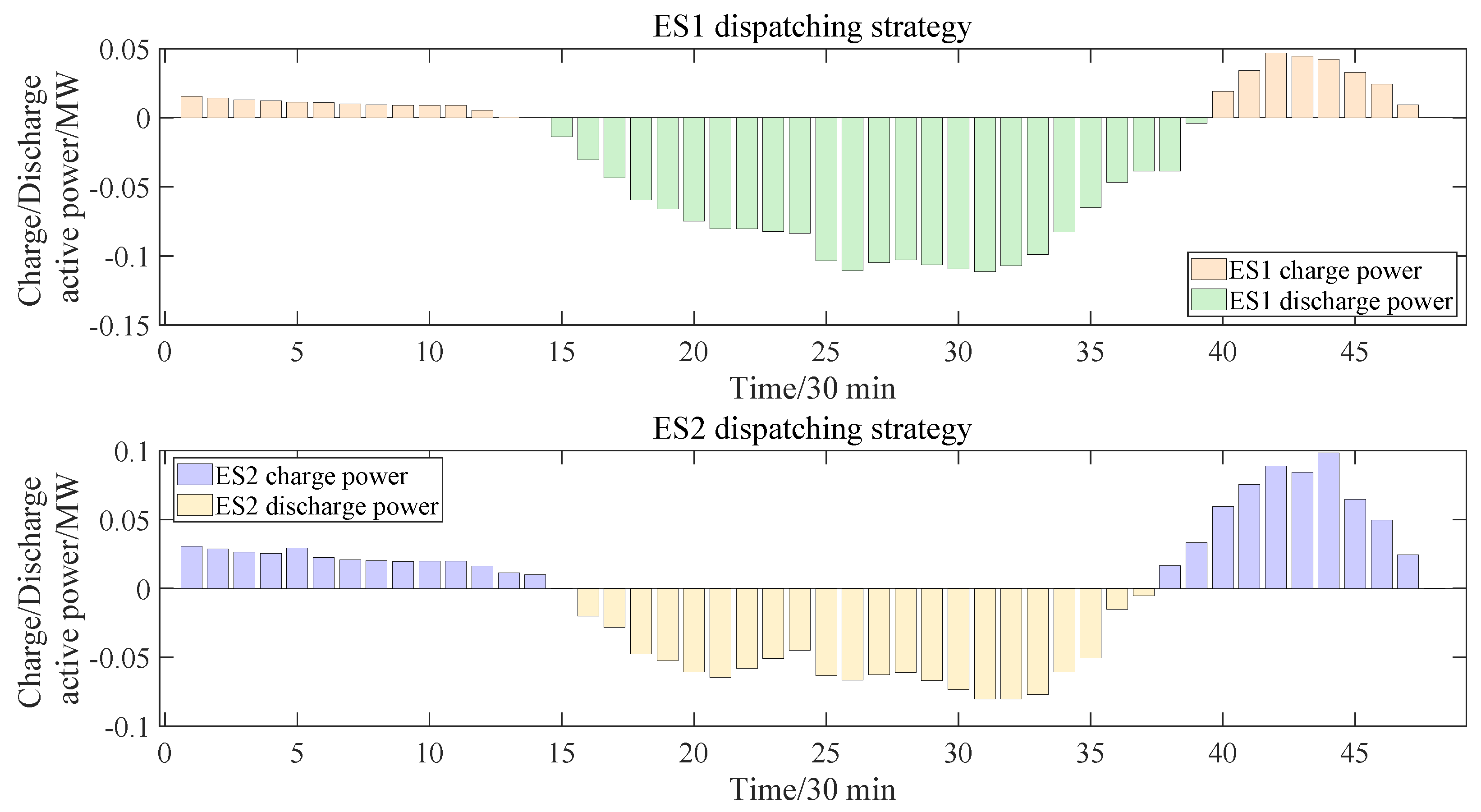
ES model

The ES model is shown in Equation (17).

$$\left\{\begin{array}{c}0\le SO{C}^t\le 1\hfill \\ s_i^t=0,P_{i,dis}^t=0,0\le P_{i,char}^t\le P_{i,max},SO{C}_i^t=SO{C}_i^{t-1}+{\displaystyle \frac{{\eta }_{i,char}{P}_{i,char}^t\Delta t}{E_{i,max}}}\hfill \\ s_i^t=1,P_{i,char}^t=0,0\le P_{i,dis}^t\le P_{i,max},SO{C}_i^t=SO{C}_i^{t-1}-{\displaystyle \frac{P_{i,dis}^t\Delta t}{{\eta }_{i,dis}{E}_{i,max}}}\hfill \end{array}\right.,t\in T=1, \dots , 48$$

(17)

where $P_{max}$ is maximum charging and discharging power of ES; $E_{max}$ is the capacity of the ES, i.e., the maximum electricity amount that the ES device store; ${\eta }_{char}$ and ${\eta }_{dis}$ are the charging and discharging efficiencies, respectively, and ${\eta }_{char},{\eta }_{dis}\in [0,1]$; $s^t$ is the ES charging and discharging state at moment t, 0 denotes charging and 1 denotes discharging; $SO{C}^t$ is the ES state of charge (SOC) at the end of moment t,and $SO{C}^t\in [0,1]$; $\Delta t=1/2$.

2.

PV inverter constraints

The PV inverter constraints are detailed in the lower-layer objective function.

3.2.2. Lower-Layer Objective Function

The lower-layer model considered three objective functions: active network loss, voltage deviation, and user benefits. The first two of them are shown in Equations (18) and (19).

1.

Active network loss

$$min{f}_1=min\sum _{t\in T}\sum _{i\in N}{R}_{ij}{\left(I_{ij}^t\right)}^2,t\in T=1, \dots , 48$$

(18)

2.

Voltage deviation

$$min{f}_2=min\sum _{t\in T}\sum _{i\in N}{(V-V_{ref})}^2,t\in T=1, \dots , 48$$

(19)

3.

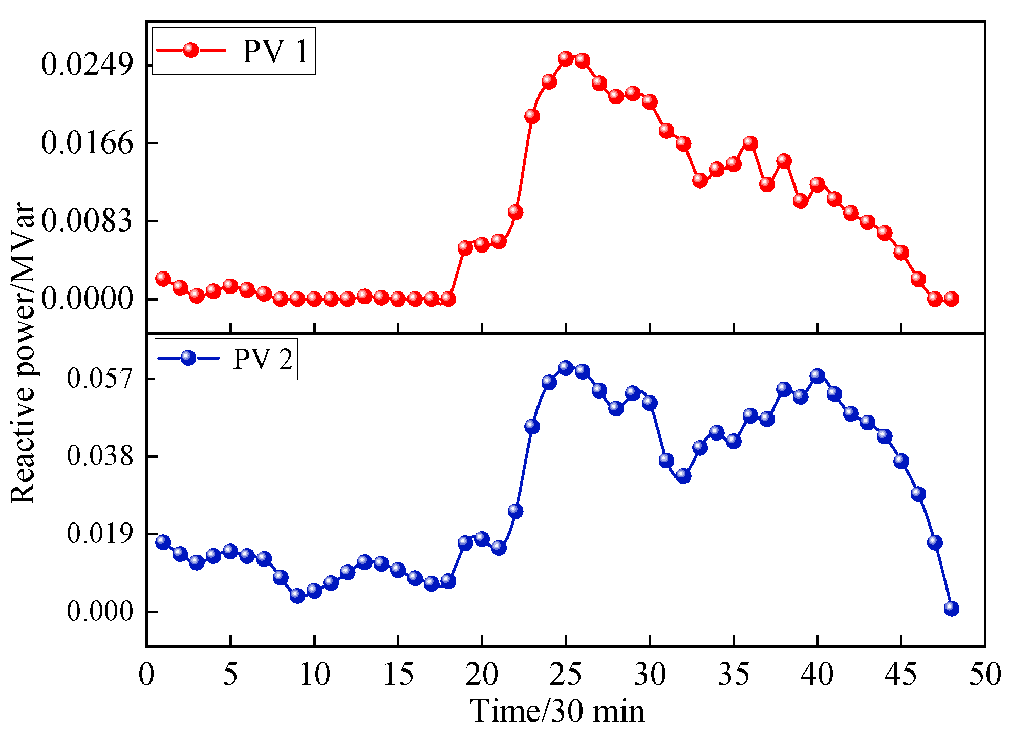
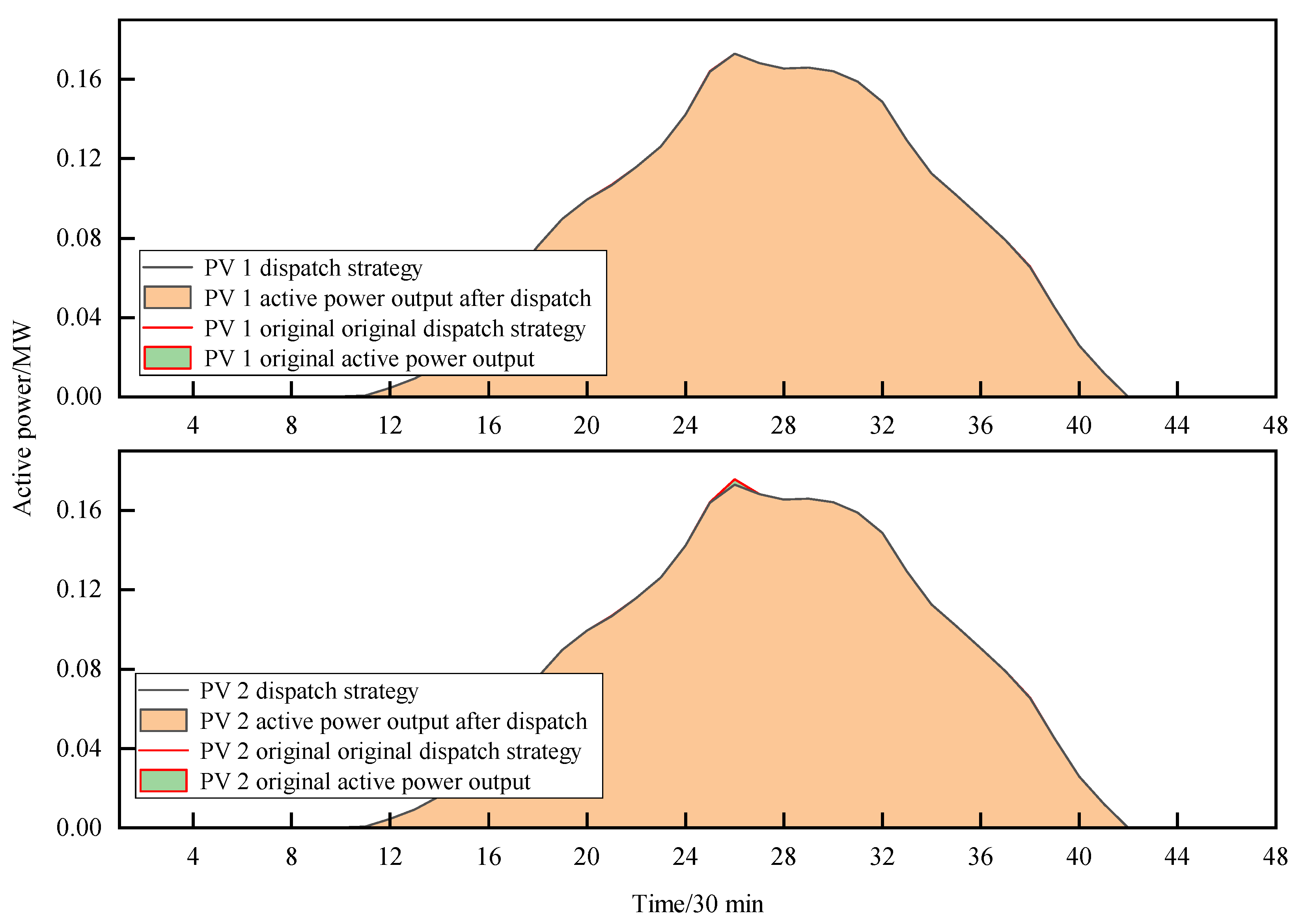
User benefits

The users benefits are ensured by adjusting PV inverters’ operating strategies. There are two PV inverter control strategies with reactive power regulation capability: RPC and OID. In practice, the operating strategy of PV inverters is maximum active power output control; therefore, the following three control strategies were considered: maximum active power output control, RPC, and OID. The principles are shown in Figure 2, the blue area is the executable region of the strategy.

The models of the three control strategies are shown in Equations (20)–(22).

$$\left\{\begin{array}{c}{Q}_{PV}=0\hfill \\ P_{PV}=P_{PV,actual\_output}\hfill \end{array}\right.$$

(20)

$$\left\{\begin{array}{c}{∥\begin{array}{c}{P}_{PV}\\ Q_{PV}\end{array}∥}_2\le S_{PV}\hfill \\ P_{PV}=P_{PV,actual\_output}\hfill \end{array}\right.$$

(21)

$$\left\{\begin{array}{c}{∥\begin{array}{c}{P}_{PV}\\ Q_{PV}\end{array}∥}_2\le S_{PV}\hfill \\ |Q_{PV}|\le P_{PV}·tan\theta \hfill \\ 0\le P_{PV}\le P_{PV,actual\_output}\hfill \end{array}\right.$$

(22)

The higher the PV active power output, the more the user benefits.

According to Figure 2, it can be seen that both control strategies (a) and (b) maximize the PV active power output in the current environment, while (c) sacrifices part of the active power output to obtain the reactive power regulation capability. Therefore, making the PV inverter switch along the sequence (a)→(b)→(c) can satisfy the objective of maximizing the PV active power output, i.e., the objective of maximizing the user benefit.

In order to obtain the above PV inverters’ control strategy ((a)→(b)→(c)), the three traditional control strategies were combined and an integrated PV inverters’ control strategy that balances active power output maximization and reactive power regulation was derived. The integrated strategy is modeled as shown in Equations (23) and (24).

$$\left\{\begin{array}{c}{∥\begin{array}{c}{P}_{i,PV}\\ Q_{i,PV}\end{array}∥}_2\le S_{i,PV}\hfill \\ 0\le P_{i,PV}\le P_{i,PV,actual\_output}\hfill \end{array}\right.$$

(23)

$$min\sum _{i\in N_{PV}}\sum _{t\in T}{(P_{i,PV,actual\_output}-P_{i,PV}^t)}^2$$

(24)

where $i\in N_{PV},t\in T=1, \dots , 48$.

Equations (23) and (24) are the constraints and user benefit objective function of the PV inverters, respectively.

The overall objective function of the lower-layer model is shown in Equation (25) and ${\sigma }_1,{\sigma }_2,{\sigma }_3$ are all taken as 0.3.

$$min{F}_2={\sigma }_1{f}_1+{\sigma }_2{f}_2+{\sigma }_3{f}_3$$

(25)

4. The Convexification of ADN Optimization Operation Model

The convexification of nonlinear models transforms them into simple ones that can be solved directly by the solver. With the application of the SOCP power-flow model, the OLTC model is changed into a nonlinear one because of the quadratic term appearance. In addition, the OLTC tap change frequency constraints and ES constraints are also nonlinear.

4.1. The Convexification of Power-Flow Model

From Equation (11), it is clear that the original branch flow model is continuously non-convex, and it can be transformed into a convex SOCP model through phase-angle relaxation, variable substitution ($v_j=V_j^2,l_{ij}=I_{ij}^2$), and second-order cone relaxation, as shown in Equation (26) [10].

$$\left\{\begin{array}{c}{∥\begin{array}{c}2P_{ij}^t\\ 2Q_{ij}^t\\ l_{ij}^t-v_{ij}^t\end{array}∥}_2\le l_{ij}^t+v_{ij}^t\hfill \\ P_j^t=\sum _{k:j\to k}{P}_{jk}^t-\sum _{i:i\to j}(P_{ij}^t-R_{ij}{l}_{ij}^t)\hfill \\ Q_j^t=\sum _{k:j\to k}{Q}_{jk}^t-\sum _{i:i\to j}(Q_{ij}^t-X_{ij}{l}_{ij}^t)\hfill \\ v_j^t=v_i^t-2(R_{ij}{P}_{ij}^t+X_{ij}{Q}_{ij}^t)+(R_{ij}^2+X_{ij}^2)l_{ij}^t\hfill \end{array}\right.$$

(26)

where $i,j\in N;(i,j),(j,k)\in L;t\in T=1, \dots , 24$.

4.2. The Linearization of OLTC Model

When applying the SOCP power-flow model, the OLTC model becomes as shown in Equation (27).

$$\left\{\begin{array}{c}{v}_1^t={\left(k^t\right)}^2\hfill \\ 0\le T^t\le K\hfill \\ k^t=\underline{V_{OLTC}}+\Delta k·T^t\hfill \end{array}\right.,t\in T=1, \dots , 24$$

(27)

where $\underline{V_{OLTC}}$ is the lower voltage limit of the OLTC secondary side.

Under the application of the SOCP power-flow model, the OLTC model becomes nonlinear; therefore, an OLTC linearization method based on binary expansion and big M method was proposed.

First, expand $T^t$ in binary. The total digit is $S+1$ and the value of the s-th digit is ${\lambda }^s$, ${\lambda }^s\in \{0,1\}$ and $S=0,1, \dots , s$, as shown in Equation (28).

$$T^t=\sum _{s=0}^S{2}^s·{\lambda }^{s,t}$$

(28)

Then, Equation (27) is transformed into Equation (29).

$$\left\{\begin{array}{c}{v}_1^t={\left(k^t\right)}^2\hfill \\ \sum _{s=0}^S{2}^s·{\lambda }^{s,t}\le K\hfill \\ k^t=\underline{V_{OLTC}}+\Delta k·\sum _{s=0}^S{2}^s·{\lambda }^{s,t}\hfill \end{array}\right.$$

(29)

Then, a new variable $y^{s,t}$ is introduced, and $y^{s,t}={\lambda }^{s,t}·k^t$. Multiply both sides of $k^t=\underline{V_{OLTC}}+\Delta k·{\sum }_{s=0}^S{2}^s·{\lambda }^{s,t}$ by $k^t$ and yield Equation (30).

$$v_1^t=\underline{V_{OLTC}}·k^t+\Delta k·\sum _{s=0}^S{2}^s·y^{s,t}$$

(30)

Afterwards, using the big M method, $y^{s,t}={\lambda }^{s,t}·k^t$ can be transformed into Equation (31).

$$\left\{\begin{array}{c}0\le y^{s,t}\le {\lambda }^{s,t}·M\hfill \\ 0\le y^{s,t}-k^t\le (1-{\lambda }^{s,t})·M\hfill \end{array}\right.$$

(31)

where the M is an arbitrarily large positive number.

Ultimately, the OLTC model is transformed into Equation (32), a mixed-integer linear one.

$$\left\{\begin{array}{c}\sum _{s=0}^S{2}^s·{\lambda }^{s,t}\le K\hfill \\ 0\le y^{s,t}\le {\lambda }^{s,t}·M\hfill \\ 0\le y^{s,t}-k^t\le (1-{\lambda }^{s,t})·M\hfill \\ v_1^t=\underline{V_{OLTC}}·k^t+\Delta k·\sum _{s=0}^S{2}^s·y^{s,t}\hfill \end{array}\right.$$

(32)

4.3. The Linearization of OLTC Operation Count Constraints

In practice, the OLTC has the limited frequency of tap change throughout the day. OLTC taps cannot be adjusted frequently and each adjustment can only be made between adjacent taps. This creates the strong coupling between time periods for the dynamic voltage/var control problem, which cannot be decoupled into a static one for each time period.

Based on the Equation (32) OLTC model, the OLTC tap-change frequency constraints are shown in Equation (33).

$$\left\{\begin{array}{c}0\le |\sum _{s=0}^S{2}^s·{\lambda }^{s,t}-\sum _{s=0}^S{2}^s·{\lambda }^{s,t-1}|\le 1\hfill \\ \sum _{t=2}^{24}|\sum _{s=0}^S{2}^s·{\lambda }^{s,t}-\sum _{s=0}^S{2}^s·{\lambda }^{s,t-1}|\le E\hfill \end{array}\right.$$

(33)

Equation (33) is a nonlinear model with absolute values. Introducing the auxiliary variable $\xi \in \{0,1\}$ and applying the big M method, Equation (33) is linearized to Equation (34).

$$\left\{\begin{array}{c}0\le Z^t\le 1\hfill \\ \sum _{t=2}^{24}{Z}^t\le E\hfill \\ 0\le Z^t-(\sum _{s=0}^S{2}^s·{\lambda }^{s,t}-\sum _{s=0}^S{2}^s·{\lambda }^{s,t-1})\le M·{\xi }^t\hfill \\ 0\le Z^t-(\sum _{s=0}^S{2}^s·{\lambda }^{s,t-1}-\sum _{s=0}^S{2}^s·{\lambda }^{s,t})\le M·(1-{\xi }^t)\hfill \end{array}\right.$$

(34)

4.4. The Linearization of the ES Model

From Equation (17), it can be seen that the charging and discharging of the ESs cannot be performed simultaneously. This lead to nonlinear constraints for both the charging and discharging power constraints and the SOC constraints.

1.

ES power constraints

The original ESs’ power constraints are shown in Equation (35). Using the idea of the big M method can linearize it. The linearized constraints are shown in Equation (36).

$$\left\{\begin{array}{c}{s}_i^t=0,P_{i,dis}^t=0,0\le P_{i,char}^t\le P_{i,max}\hfill \\ s_i^t=1,P_{i,char}^t=0,0\le P_{i,dis}^t\le P_{i,max}\hfill \end{array}\right.$$

(35)

$$\left\{\begin{array}{c}0\le P_{i,dis}^t\le s_i^t·P_{i,max}\hfill \\ 0\le P_{i,char}^t\le (1-s_i^t)·P_{i,max}\hfill \end{array}\right.$$

(36)

2.

ES SOC constraints

The original ESs SOC constraints are shown in Equation (37). Using the big M method can linearize it. The linearized constraints is shown in Equation (38).

$$\left\{\begin{array}{c}{s}_i^t=1,SO{C}_i^t=SO{C}_i^{t-1}-{\displaystyle \frac{P_{i,dis}^t\Delta t}{{\eta }_{i,dis}{E}_{i,max}}}\hfill \\ s_i^t=0,SO{C}_i^t=SO{C}_i^{t-1}+{\displaystyle \frac{{\eta }_{i,char}{P}_{i,char}^t\Delta t}{E_{i,max}}}\hfill \end{array}\right.$$

(37)

$$\left\{\begin{array}{c}SO{C}_i^{t-1}+{\displaystyle \frac{{\eta }_{i,char}{P}_{i,char}^t\Delta t}{E_{i,max}}}-s_i^t·M\le SO{C}_i^t\le SO{C}_i^{t-1}+{\displaystyle \frac{{\eta }_{i,char}{P}_{i,char}^t\Delta t}{E_{i,max}}}+s_i^t·M\hfill \\ SO{C}_i^{t-1}-{\displaystyle \frac{P_{i,dis}^t\Delta t}{{\eta }_{i,dis}{E}_{i,max}}}-(1-s_i^t)·M\le SO{C}_i^t\le SO{C}_i^{t-1}-{\displaystyle \frac{P_{i,dis}^t\Delta t}{{\eta }_{i,dis}{E}_{i,max}}}+(1-s_i^t)·M\hfill \end{array}\right.$$

(38)

The Equation (39) constraints ensure that in the charging state ($s^t=0$), only the charge SOC is valid while the discharge SOC is not; and in the discharging state ($s^t=1$), only the discharge SOC is valid while the charge SOC is not.

$$0\le SO{C}^t\le 1$$

(39)

Therefore, the linearized ESs model combined with Equations (36), (38), and (39), i.e., a mixed-integer linear model.

5. Case Study

IEEE33 node radial distribution network and Matlab 2022b were used in the case study.

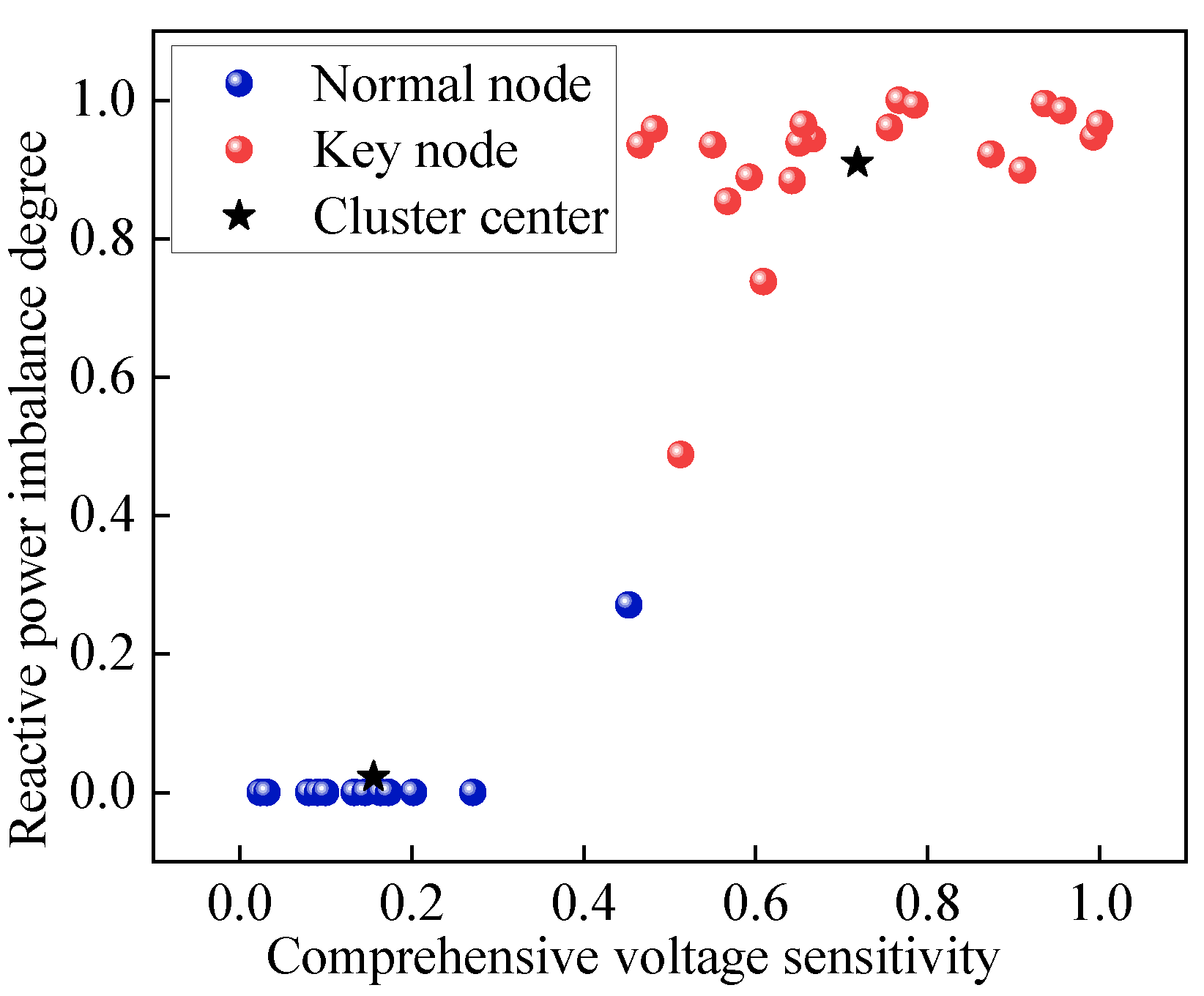
5.1. “Key” Nodes Selection

The results of “key” nodes selection are shown in Figure 3, the red dots indicate “key” nodes, the blue dots indicate “normal” nodes, and the asterisks are the clustering centers. It can be seen that the improved K-means clustering algorithm has a good classification effect. The “key” nodes are 6, 7, 8, 9, 10, 11, 12, 13, 14, 15, 16, 18, 25, 26, 27, 28, 29, 30, 31, 32.

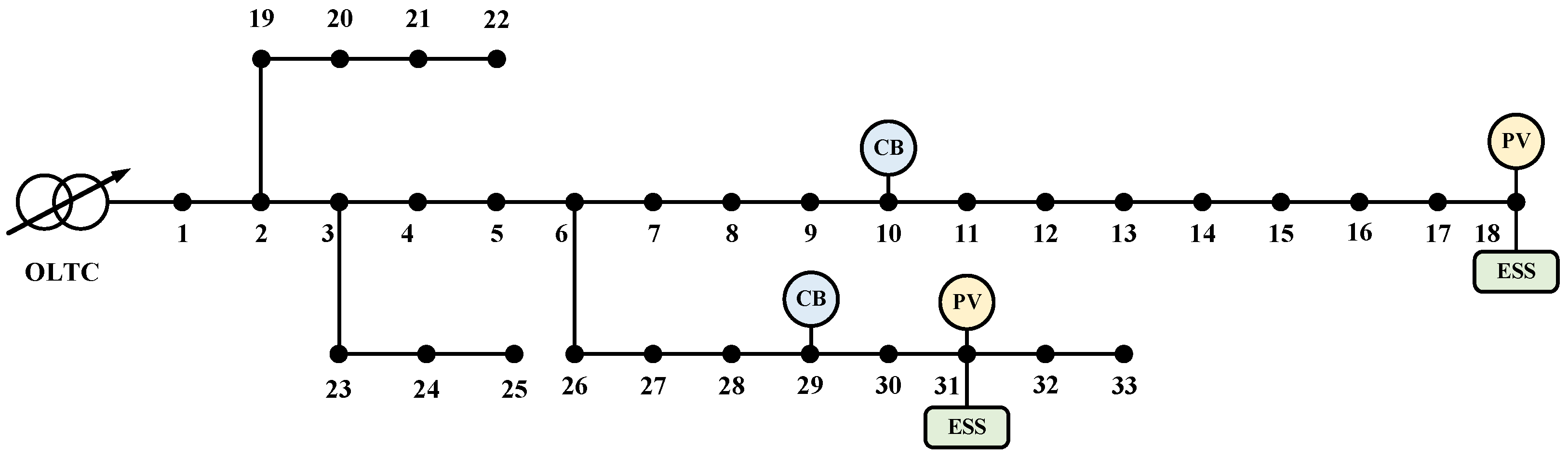
5.2. Case Allocation

We configured IEEE33 distribution network system by integrating the proposed improved K-means algorithm with practical insights. Initially, an improved K-means clustering algorithm pinpointed candidate key nodes. Then, informed by the radial distribution network’s features and practical experience, further selections were made. In radial distribution networks, voltage drops progressively from head-end nodes near the generator to distant ones. To ensure voltage quality across the distribution network, we installed reactive power CBs, PVs, and ESs at mid-nodes and ends of main line and long branch.

The case allocation involves configuring PV according to high penetration situation. The number of the PVs is two, both capacities are 1800 kW, the total capacity is 3600 kW, connected to node 18 and node 31, respectively. The number of the CBs is two, connected to node 10 and node 29, respectively, and their capacities are 1300 kVar and 1000 kVar, respectively. Both CBs have 10 banks and each bank’s capacities are 130 kVar and 100 kVar, respectively. The OLTC is connected to node 1. It has 5 taps, the step between two taps is 2.5%; so, the OLTC voltage regulation range is 0.95–1.05 p.u. The number of the distributed ESs is two, connected to node 18 and node 31, respectively; their capacities are both 13 MW and their maximum charging and discharging power are both 1.7 MW.

The case allocation is in Figure 4.

5.3. Curves for Load and PV Active-Power Output

The 24 h active and reactive load curves are shown in Figure 5, and their projections demonstrate the trend of their values over time and over nodes.

From the figures, it can be seen that the active load connected to node 24 is maximum while the reactive load connected to node 30 is maximum. During the day, there are two peaks for both active and reactive loads, the two peaks for active loads are at the 14 and 21 moments, respectively, and the two peaks for reactive loads are at the 13 and 20 moments, respectively.

The 24 h original PV active power output curve (each PV) is shown in Figure 6.

It can be seen that the peak PV active power output moment is around the 13th moment, and there are about 9 h in a day when the PV active power output is zero.

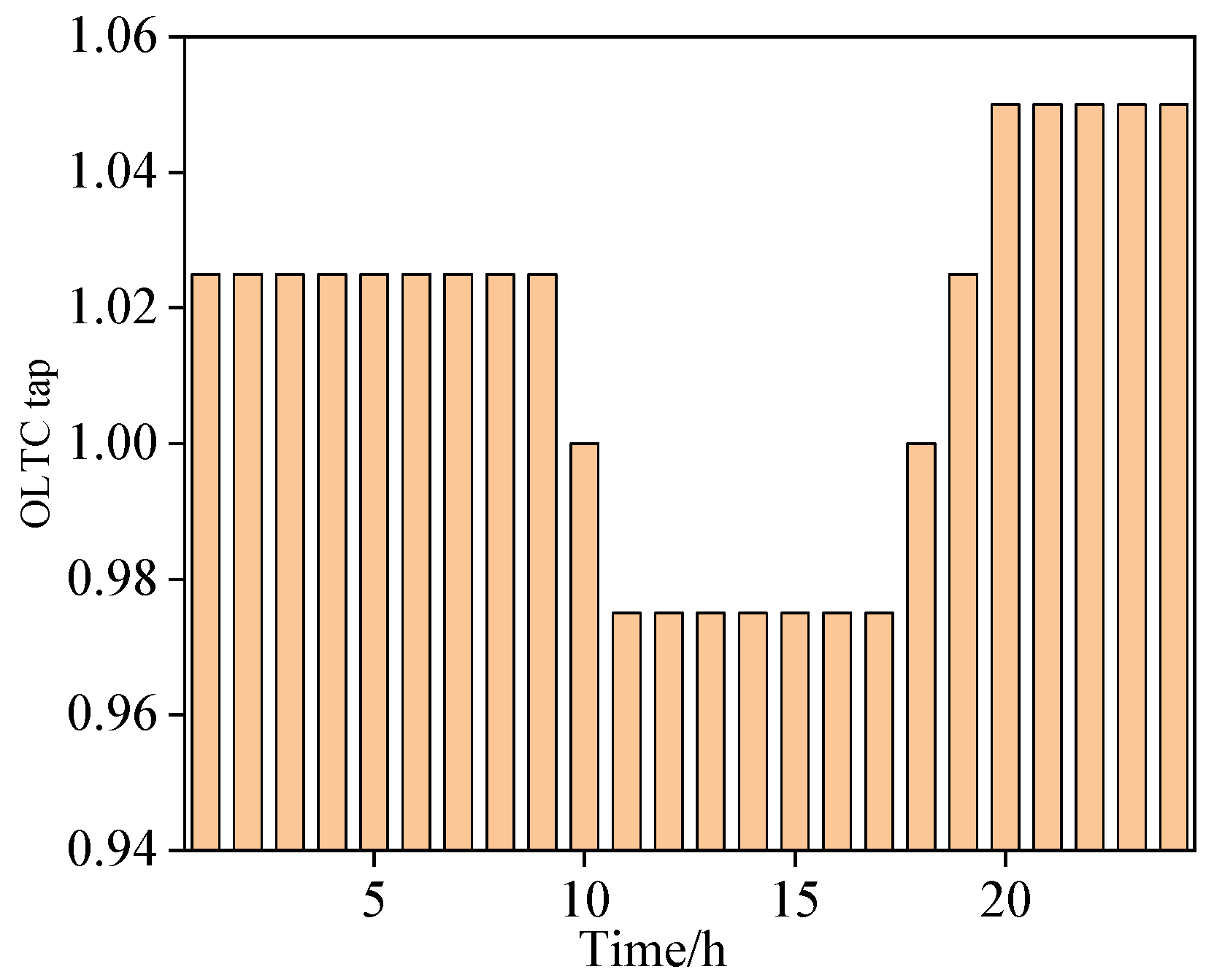
5.4. Upper-Layer Equipment-Dispatching Strategies

The OLTC dispatching strategy is shown in Figure 7.

It can be seen from the figure, the low-voltage-side voltages of the OLTC are in the range of 0.975 p.u.–1.025 p.u. and lie between the lower limit of 0.95 p.u. and the upper limit of 1.05 p.u. The number of tap adjustments in a day is 6.

Tap adjustments between adjacent moments are continuous, and tap adjustments between the 1st and 24th moments are also continuous. All of them meet the OLTC operation requirements.

The dispatching strategy of the two CBs are shown in Figure 8.

It can be seen that the first compensation small peak occurs around the 11th moment and the second compensation small peak occurs around the 16th moment. This is because the load is high at these two moments and the reactive power compensation is increased to ensure that the voltages are within the qualified range.

5.5. Lower-Layer Equipment-Dispatching Strategies

The generator active power output curve of the day at the first end of ADN is shown in Figure 9.

It can be seen that the generator active output has two peaks near the 13th moment and 20th moment respectively, roughly coinciding with the two peak moments of the load curve. Excessive PV power generation is likely to result in power-flow reverse. When power-flow reverse occurs, generators may experience negative power output. This phenomenon is not in line with normal operating principles. It disrupts the stable operation of power systems, and can even trigger safety issues. After the proposed strategy, the generators did not exhibit a negative power output. This indicates that the rational operation requirements of the ADN are met, contributing to stable operation and reliable power supply of the active distribution network.

The dispatching strategies for ESs are shown in Figure 10.

It can be seen that at peak moments the ESs discharge to meet load demand; the rest of the time they charge. The discharging power of ES1 exceeds its charging power can likely be attributed to the relatively heavy load near the node where ES1 is connected. As a crucial power-supplementation source, ES1 is required to release more electrical energy to meet the load demand. In contrast, for Energy Storage 2 (ES2), the similar magnitudes of its charging and discharging powers may stem from the lighter load near the node it is connected to. ES2 mainly serves a fine-tuning function in maintaining the power balance of the distribution network. The reason may be that the load near the node where ES2 is connected is relatively light, and ES2 mainly plays a role in fine-tuning.

The PVs reactive power output dispatching strategies are shown in Figure 11.

It can be seen that the PVs’ curve of reactive-power output is similar to the CBs reactive power output. Both of them have two peaks near the 13th moment and 20th moment, which are capable of meeting the load demand while satisfying the voltage qualification.

The PVs’ active-power output of the day before and after dispatching is shown in Figure 12.

This proves that the PV inverters are actively and continuously playing the role of reactive-power regulation. It can also be seen that before and after dispatching, the active-power output of the PVs is almost unchanged. This is the result of pursuing the maximum PVs active output to ensure the users’ interests. Therefore, the results of the dispatching are satisfactory.

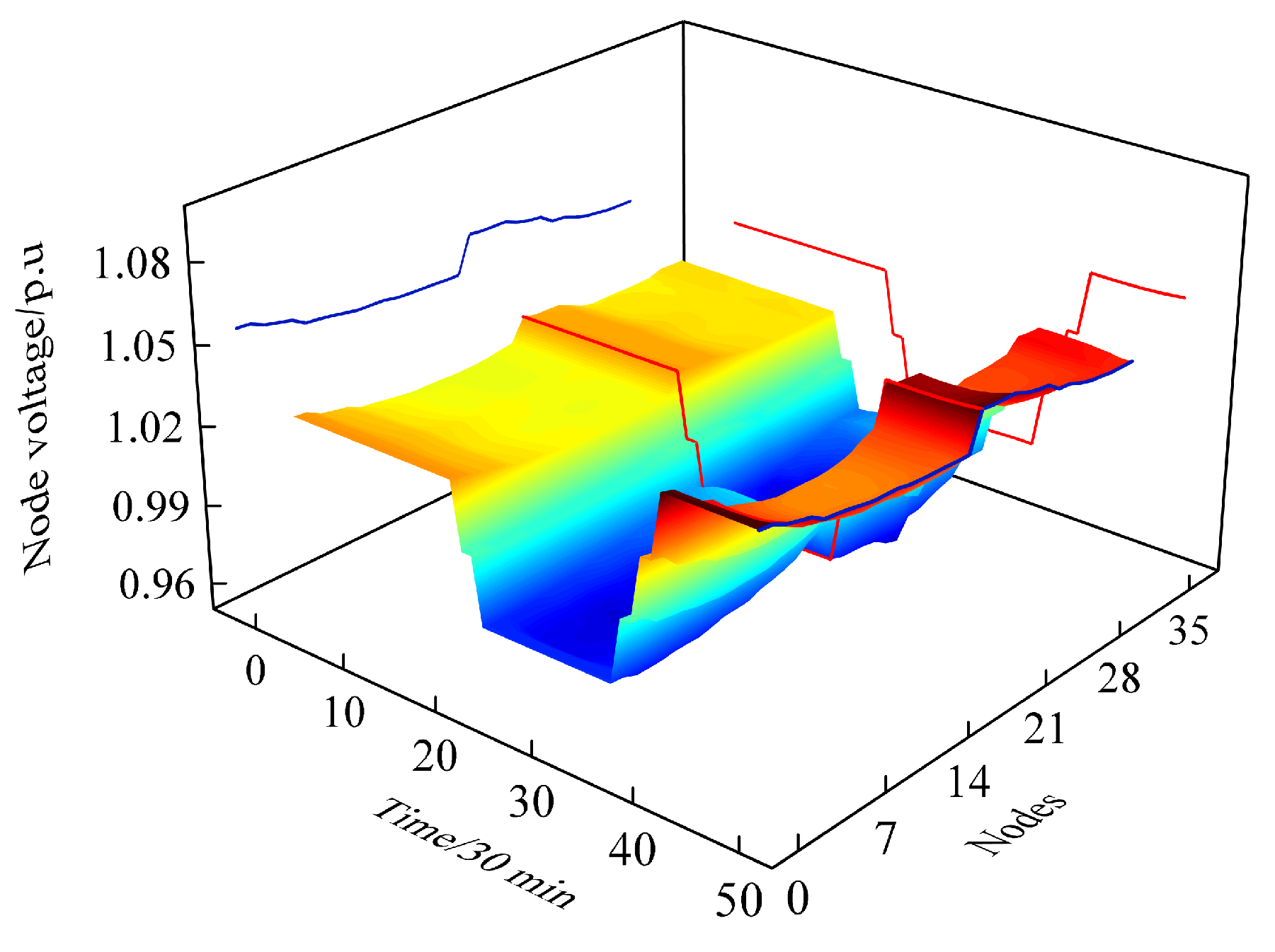
5.6. Optimal Dispatching Results

The network loss before optimal dispatching is 1.355 MW, and the network loss after optimal dispatching is 336.077 kW, decreased by 75.20%. It shows that the optimization effect for network loss is obvious.

The node voltages of the ADN are shown in the Figure 13, and its projections show the trend of voltage values over time and over nodes.

It can be seen that the all node voltages specification is between 0.95 p.u. and 1.05 p.u., which are all within the qualified range. In addition, from the perspective of time, it also can be seen that the trend of the node voltages is the same as that of OLTC. This means that the OLTC has a great influence on the node voltages.

6. Conclusions

In order to solve the problem of ADN increased dispatching difficulty caused by the high DG penetration, this paper proposed a two-layer optimal dispatching model for ADN based on convex optimization. Firstly, the active–reactive voltage sensitivity and reactive power-balance degree were introduced as comprehensive indexes, and the “key” nodes were selected using the improved K-means clustering method. Then, a two-layer optimization model was established based on the different time scales. The upper-layer model is a long-time-scale one, contains OLTC and CBs. The lower-layer model is a short-time-scale one, contains PV inverters and ESs. In addition, by proposing the PV inverters’ comprehensive control strategy, the model also took into account the users’ benefits. Afterwards, the linearization methods were proposed for OLTC model and its operation constraints model, and the two-layer model was eventually transformed into a MISOC model. Finally, the effectiveness of the proposed method was verified by solving the improved IEEE33 case using the CPLEX solver and the following conclusions were drawn:

1.

The proposed OLTC linearization method did convert the non-linear OLTC model into linear one under the application of the SOCP power-flow mode, and the proposed OLTC tap-change frequency constraints linearization method made the OLTC model more practical;

2.

The proposed PV inverters control strategy enabled voltage/var control while simultaneously ensuring user benefits;

3.

The proposed comprehensive “key” node selection indexes and the proposed improved K-means algorithm increased the reliability of key node selection;

4.

The proposed two-layer optimization model has led to a 70% reduction in network losses and has successfully maintained all node voltages within qualified limits. This demonstrates that the proposed method is beneficial for both the economic and stable operation of the distribution network.

The proposed model transforms common non-linear device models in the ADN into linear or convex ones. This enables solving ADN optimal operation problems with solvers like Cplex, simplifying the process. Even when applied to complex ADNs with numerous non-linear devices, the model simplifies problem solving through such conversions.

However, as ADNs develop, more complex non-linear devices are being connected. Thus, there is a need to enhance the proposed model. This shows the current model has limitations in dealing with emerging complex non-linear devices. Considering ADNs’ future development, the growing complexity may also impact the model’s computational complexity and real-time applicability.

References

- Mehrjerdi, H.; Hemmati, R.; Farrokhi, E. Nonlinear stochastic modeling for optimal dispatch of distributed energy resources in active distribution grids including reactive power. Simul. Model. Pract. Theory 2019, 94, 1–13. [Google Scholar] [CrossRef]
- Kerrouche, S.; Djerioui, A.; Zeghlache, S.; Houari, A.; Saim, A.; Rezk, H.; Benkhoris, M.F. Integral backstepping-ILC controller for suppressing circulating currents in parallel-connected photovoltaic inverters. Simul. Model. Pract. Theory 2023, 123, 102706. [Google Scholar] [CrossRef]
- Song, J.; Jung, S.; Lee, J.; Shin, J.; Jang, G. Dynamic performance testing and implementation for static var compensator controller via hardware-in-the-loop simulation under large-scale power system with real-time simulators. Simul. Model. Pract. Theory 2021, 106, 102191. [Google Scholar] [CrossRef]
- Wang, J.; Yao, L.; Liang, J.; Wang, J.; Cheng, F. Distributed optimization strategy for networked microgrids based on network partitioning. Appl. Energy 2025, 378, 124834. [Google Scholar] [CrossRef]
- Ding, T.; Li, C.; Yang, Y.; Jiang, J.; Bie, Z.; Blaabjerg, F. A two-stage robust optimization for centralized-optimal dispatch of photovoltaic inverters in active distribution networks. IEEE Trans. Sustain. Energy 2016, 8, 744–754. [Google Scholar] [CrossRef]
- Emiliano, D.; Sairaj, V.; Brian, G.; Georgios, B. Optimal dispatch of residential photovoltaic inverters under forecasting uncertainties. IEEE J. Photovoltaics 2014, 5, 350–359. [Google Scholar]
- Emiliano, D.; Sairaj, V.; Brian, G.; Georgios, B. Decentralized optimal dispatch of photovoltaic inverters in residential distribution systems. IEEE Trans. Energy Convers. 2014, 29, 957–967. [Google Scholar]
- González-Moreno, A.; Marcos, J.; Parra, I.; Marroyo, L. Control method to coordinate inverters and batteries for power ramp-rate control in large PV plants: Minimizing energy losses and battery charging stress. J. Energy Storage 2023, 72, 108621. [Google Scholar] [CrossRef]
- Luo, L.; Gu, W.; Zhang, X.-P.; Cao, G.; Wang, W.; Zhu, G.; You, D.; Wu, Z. Optimal siting and sizing of distributed generation in distribution systems with PV solar farm utilized as STATCOM (PV-STATCOM). Appl. Energy 2018, 210, 1092–1100. [Google Scholar] [CrossRef]
- Masoud, F.; Steven, H.L. Branch flow model: Relaxations and convexification—Part I. IEEE Trans. Power Syst. 2013, 28, 2554–2564. [Google Scholar]
- Masoud, F.; Steven, H.L. Branch flow model: Relaxations and convexification—Part II. IEEE Trans. Power Syst. 2013, 28, 2565–2572. [Google Scholar]
- Wang, Z.; Kirschen, D.S.; Zhang, B. Accurate semidefinite programming models for optimal power flow in distribution systems. arXiv 2017, arXiv:1711.07853. [Google Scholar]
- Gan, L.; Low, S.H. Convex relaxations and linear approximation for optimal power flow in multiphase radial networks. In Proceedings of the 2014 Power Systems Computation Conference, Wroclaw, Poland, 18–22 August 2014; pp. 1–9. [Google Scholar]
- Wu, W.; Tian, Z.; Zhang, B. An exact linearization method for OLTC of transformer in branch flow model. IEEE Trans. Power Syst. 2016, 32, 2475–2476. [Google Scholar] [CrossRef]
- Wolsey, L.A.; Nemhauser, G.L. Integer and Combinatorial Optimization; John Wiley & Sons: Hoboken, NJ, USA, 1999. [Google Scholar]
- Bazaraa, M.S.; Jarvis, J.J.; Sherali, H.D. Linear Programming and Network Flows; John Wiley & Sons: Hoboken, NJ, USA, 2011. [Google Scholar]
- Dasgupta, S.; Baral, A.; Lahiri, A. Optimization of Electric Stress in a Vacuum Interrupter Using Charnes’ Big M Algorithm. IEEE Trans. Dielectr. Electr. Insul. 2022, 30, 877–882. [Google Scholar] [CrossRef]
- Ye, K.; Zhao, J.; Huang, C.; Duan, N.; Zhang, Y.; Field, T.E. A data-driven global sensitivity analysis framework for three-phase distribution system with PVs. IEEE Trans. Power Syst. Trans. Power Syst. 2021, 36, 4809–4819. [Google Scholar]
- Rubén J, S.; Max, F.; Seán, N.; Nick, W.; Graham, N.; Jacek, B.; Janusz, W.B. Hierarchical spectral clustering of power grids. IEEE Trans. Power Syst. 2014, 29, 2229–2237. [Google Scholar]
- Di, S.; Daniel, J.T. A novel bus-aggregation-based structure-preserving power system equivalent. IEEE Trans. Power Syst. 2014, 30, 1977–1986. [Google Scholar]
- Zhao, B.; Xu, Z.; Xu, C.; Wang, C.; Lin, F. Network partition-based zonal voltage control for distribution networks with distributed PV systems. IEEE Trans. Smart Grid 2017, 9, 4087–4098. [Google Scholar]
- Meng, L.; Yang, X.; Zhu, J.; Wang, X.; Meng, X. Network partition and distributed voltage coordination control strategy of active distribution network system considering photovoltaic uncertainty. Appl. Energy 2024, 362, 122846. [Google Scholar]
- Ma, L.; Wang, L.; Liu, Z. Self-organized partition of distribution networks with distributed generations and soft open points. Electr. Power Syst. Res. 2022, 208, 107910. [Google Scholar]
- Li, Y.; Liu, C.; Zhang, L.; Sun, B. A partition optimization design method for a regional integrated energy system based on a clustering algorithm. Energy 2021, 219, 119562. [Google Scholar] [CrossRef]
- Wang, Y.; Ma, J.; Gao, N.; Wen, Q.; Sun, L.; Guo, H. Federated fuzzy k-means for privacy-preserving behavior analysis in smart grids. Appl. Energy 2023, 331, 120396. [Google Scholar] [CrossRef]
- Zhu, Z.; Zeng, F.; Qi, G.; Li, Y.; Jie, H.; Mazur, N. Power system structure optimization based on reinforcement learning and sparse constraints under DoS attacks in cloud environments. Simul. Model. Pract. Theory 2021, 110, 102272. [Google Scholar] [CrossRef]
- Manzoor, A.; Judge, M.A.; Ahmed, F.; ul Islam, S.; Buyya, R. Towards simulating the constraint-based nature-inspired smart scheduling in energy intelligent buildings. Simul. Model. Pract. Theory 2022, 118, 102550. [Google Scholar] [CrossRef]
- Suryakiran, B.; Nizami, S.; Verma, A.; Saha, T.; Mishra, S. A DSO-based day-ahead market mechanism for optimal operational planning of active distribution network. Energy 2023, 282, 128902. [Google Scholar] [CrossRef]
- Xiang, Y.; Lu, Y.; Liu, J. Deep reinforcement learning based topology-aware voltage regulation of distribution networks with distributed energy storage. Appl. Energy 2023, 332, 120510. [Google Scholar] [CrossRef]
- Miguel, P.; Lukas, O.; Saverio, B.; Florian, D. Adaptive real-time grid operation via online feedback optimization with sensitivity estimation. Electr. Power Syst. Res. 2022, 212, 108405. [Google Scholar]
- Jochen, S.; Thierry, Z.; Giacomo, P.; Damiano, T.; Gabriela, H.; Konstantinos, B. Sensitivity analysis of electric vehicle impact on low-voltage distribution grids. Electr. Power Syst. Res. 2021, 191, 106696. [Google Scholar]
- Pierrou, G.; Wang, X. An online network model-free wide-area voltage control method using PMUs. IEEE Trans. Power Syst. 2021, 36, 4672–4682. [Google Scholar] [CrossRef]
- Elshahed, M.; Tolba, M.A.; El-Rifaie, A.M.; Ginidi, A.; Shaheen, A.; Mohamed, S.A. An artificial rabbits’ optimization to allocate PVSTATCOM for ancillary service provision in distribution systems. Mathematics 2023, 11, 339. [Google Scholar] [CrossRef]
- González-Cabrera, N.; Ortiz-Bejar, J.; Zamora-Mendez, A.; Paternina Mario, R.A. On the Improvement of representative demand curves via a hierarchical agglomerative clustering for power transmission network investment. Energy 2021, 222, 119989. [Google Scholar] [CrossRef]
Disclaimer/Publisher’s Note: The statements, opinions and data contained in all publications are solely those of the individual author(s) and contributor(s) and not of MDPI and/or the editor(s). MDPI and/or the editor(s) disclaim responsibility for any injury to people or property resulting from any ideas, methods, instructions or products referred to in the content. |
© 2025 by the authors. Licensee MDPI, Basel, Switzerland. This article is an open access article distributed under the terms and conditions of the Creative Commons Attribution (CC BY) license (https://creativecommons.org/licenses/by/4.0/).
Share and Cite
Shi, J.; Hu, S.; Fu, R.; Zhang, Q. Convex Optimization and PV Inverter Control Strategy-Based Research on Active Distribution Networks. Energies 2025, 18, 1793. https://doi.org/10.3390/en18071793
Shi J, Hu S, Fu R, Zhang Q. Convex Optimization and PV Inverter Control Strategy-Based Research on Active Distribution Networks. Energies. 2025; 18(7):1793. https://doi.org/10.3390/en18071793
Chicago/Turabian StyleShi, Jiachuan, Sining Hu, Rao Fu, and Quan Zhang. 2025. "Convex Optimization and PV Inverter Control Strategy-Based Research on Active Distribution Networks" Energies 18, no. 7: 1793. https://doi.org/10.3390/en18071793
APA StyleShi, J., Hu, S., Fu, R., & Zhang, Q. (2025). Convex Optimization and PV Inverter Control Strategy-Based Research on Active Distribution Networks. Energies, 18(7), 1793. https://doi.org/10.3390/en18071793