Abstract
In transmission lines, the discharge characteristics of long air gaps significantly influence the design of external insulation. Existing machine learning models for predicting breakdown voltage are typically limited to single gaps and do not account for the combined effects of complex factors. To address this issue, this paper proposes a novel prediction model based on the Improved Sparrow Search Algorithm-optimized XGBoost (ISSA-XGBoost). Initially, a comprehensive dataset of 46-dimensional electric field eigenvalues was extracted for each gap using finite element simulation software and MATLAB. Subsequently, the model incorporated a comprehensive set of input variables, including electric field eigenvalues, gap distance, waveform and polarity of the switching impulse voltage, temperature, relative humidity, and atmospheric pressure. After training, the ISSA-XGBoost model achieved a Mean Absolute Percentage Error (MAPE) of 7.85%, a Root Mean Squared Error (RMSE) of 56.92, and a Coefficient of Determination (R2) of 0.9938, indicating high prediction accuracy. In addition, the ISSA-XGBoost model was compared with traditional machine learning models and other optimization algorithms. These comparisons further substantiated the efficacy and superiority of the ISSA-XGBoost model. Notably, the model demonstrated exceptional performance in terms of predictive accuracy under extreme atmospheric conditions.
1. Introduction
In transmission lines, long air gaps serve as the predominant form of external insulation. Their discharge characteristics are crucial for the design of external insulation in transmission and transformation projects, and they are influenced by a multitude of factors, including electrode structure, voltage type, and atmospheric conditions [1]. Rod/sphere–plate and rod–rod gaps are typical gap configurations, each exhibiting distinct discharge voltage characteristics [2,3,4]. Consequently, investigating the discharge characteristics of these various gap structures is not only representative, but also holds significant value for practical engineering applications. Due to the immature nature of discharge theory, the acquisition of breakdown voltage still relies heavily on specific gap discharge experiments. However, full-scale experiments are costly and time-consuming. To address these issues, researchers are actively exploring the mechanisms and models of gap discharge, employing a combination of experimental and simulation methods to reduce the workload associated with external insulation design. Currently, the computational models for air gap breakdown voltage primarily consist of empirical formulas [5], semi-empirical formulas [6], and physical models [7]. Among these, empirical and semi-empirical formulas are relatively straightforward and are more frequently applied in practical engineering. However, some parameters within these formulas are derived under specific conditions, limiting their general applicability. Owing to the current inadequacies in observational methods and theoretical research on gap discharge, the results obtained from physical models often exhibit considerable discrepancies compared to experimental values.
To overcome the limitations of the traditional methods of obtaining gap breakdown voltage, some scholars have proposed a research approach that combines machine learning algorithms with high-voltage science. This approach is based on high-voltage experiments and utilizes machine learning models to process the complex relationships between multiple factors. By incorporating electric field features [8] that influence air discharge, voltage waveforms and polarities [9], and atmospheric parameters [10] as input variables, the model is trained to establish a multidimensional nonlinear relationship between these inputs and the breakdown voltage, thereby enabling the prediction of breakdown voltage. The traditional experimental methods often require substantial time and resources to collect data and struggle to account for all possible factors that may affect breakdown voltage. In contrast, machine learning models can automatically identify key factors and establish their complex relationships by inputting and analyzing extensive datasets. Even in the absence of a complete dataset, the model can make reasonable predictions based on the available data.
In the process of obtaining the breakdown voltage of long air gaps, accurately describing the three-dimensional structure of the gap presents a significant challenge. Relying solely on geometric parameters such as electrode dimensions and gap distance fails to fully capture the rich three-dimensional spatial characteristics of the gap, particularly when data are limited, leading to reduced prediction accuracy of the model. To address this issue, various methods have been employed to enhance the precision of breakdown voltage prediction. Reference [11] utilized simulations to construct the conical electric field region and the shortest path between electrodes, extracting electric field features as model inputs and employing Support Vector Machines (SVM) for breakdown voltage prediction. Reference [12] focused on using electrostatic field characteristics to describe the gap structure, directly analyzing the nonlinear relationship between electric field features and breakdown voltage, which was a relatively straightforward approach. Reference [13] combined electric field characteristics with impulse voltage waveform characteristics to represent the energy storage state of the air gap, using these as input variables for SVM, achieving favorable prediction results. However, most of the aforementioned studies did not consider the coupled effects of complex factors such as voltage waveform, polarity, and atmospheric parameters. Regarding the impact of atmospheric parameters, reference [14] adopted an improved neural network algorithm, incorporating gap distance and atmospheric parameters as input variables, demonstrating good predictive capability for breakdown voltage. However, this study only included experimental data for rod–plate long air gaps and did not encompass other types of gap structures, nor did it consider variations in voltage waveform and polarity, thus limiting its general applicability.
To address the limitations of previous research, this paper introduced an XGBoost model optimized by an Improved Sparrow Search Algorithm (ISSA). The main contributions of this paper were as follows:
- (1)
- This paper meticulously assembled a comprehensive dataset comprising 373 distinct sets of breakdown voltage measurements under switching impulse voltage for various long air gap configurations, specifically including rod/sphere–plate and rod–rod arrangements. The research was endowed with an ample and diverse array of data, thereby facilitating an in-depth and multifaceted analysis of the gap types;
- (2)
- This paper employed electric field characteristics, gap distance, and waveform and polarity of switching impulse voltage, as well as atmospheric parameters such as input variables for the predictive model. It thoroughly investigated the intricate interdependencies among the various factors influencing the breakdown voltage of long air gaps, thereby enhancing the robust applicability of the model;
- (3)
- Addressing the issue of potential local optima in the later iterations of the Sparrow Search Algorithm, this paper introduced elite and memory strategies to refine the algorithm. The Improved Sparrow Search Algorithm demonstrated significant efficacy in optimizing the hyperparameters of the XGBoost model;
- (4)
- Utilizing the ISSA-XGBoost model, this study predicted the switching impulse breakdown voltage for rod/sphere–plate and rod–rod long air gaps, achieving a relatively small prediction error. The results were compared with those from traditional machine learning models and other optimization algorithms, thereby substantiating the effectiveness and superiority of the proposed model.
2. Data
In this section, we delineated the dataset utilized in the model training and test process and elucidated the categories and significance of the model’s input variables.
2.1. Source
This paper focused on the study of typical long air gaps, with the data sources presented in Table 1. The dataset comprised a total of 373 data points, encompassing both rod/sphere–plate and rod–rod gap configurations [15,16,17,18,19,20,21,22,23,24,25].

Table 1.
Introduction of the dataset.
The dataset encompasses a multitude of influencing factors, including various gap configurations, gap distances, and applied voltage waveforms and polarities, as well as atmospheric parameters.
2.2. Model Input Variables
The discharge phenomena of rod/sphere–plate and rod–rod long air gaps are the result of interactions among multiple physical fields, influenced by various factors such as gap structure, voltage waveform, voltage polarity, and atmospheric conditions. To construct a predictive model, this paper extracted the following key features as input variables:
- (1)
- Electric field eigenvalues: The breakdown voltage of long air gaps is significantly affected by the gap structure, which primarily includes gap distance and electrode dimensions. Utilizing finite element simulation software in conjunction with MATLAB, this paper extracted electric field features for different gap configurations. These features encompassed the electric field strength and its rate of change in both horizontal and vertical directions, as well as electric field energy and energy density;
- (2)
- Characteristics of switching impulse voltage: Under switching impulse voltage, the waveform exerts a pronounced influence on gap discharge. Additionally, due to the differences in the discharge processes of positive and negative polarity gaps, voltage polarity also impacts the magnitude of the breakdown voltage;
- (3)
- Atmospheric parameters: When conducting gap discharge experiments, environmental conditions such as temperature, humidity, and atmospheric pressure are typically recorded. These atmospheric factors also exert a significant influence on the breakdown voltage of air gaps.
The following data preprocessing steps were carried out: First, feature scaling was performed to standardize the features, transforming them to have a mean of 0 and a standard deviation of 1. By doing so, we aimed to bring all of the features to a comparable scale. Next, for feature selection, all features were retained to fully account for the coupling effects among the different features.
3. Methodology
3.1. ISSA-XGBoost
3.1.1. Model Prediction Process
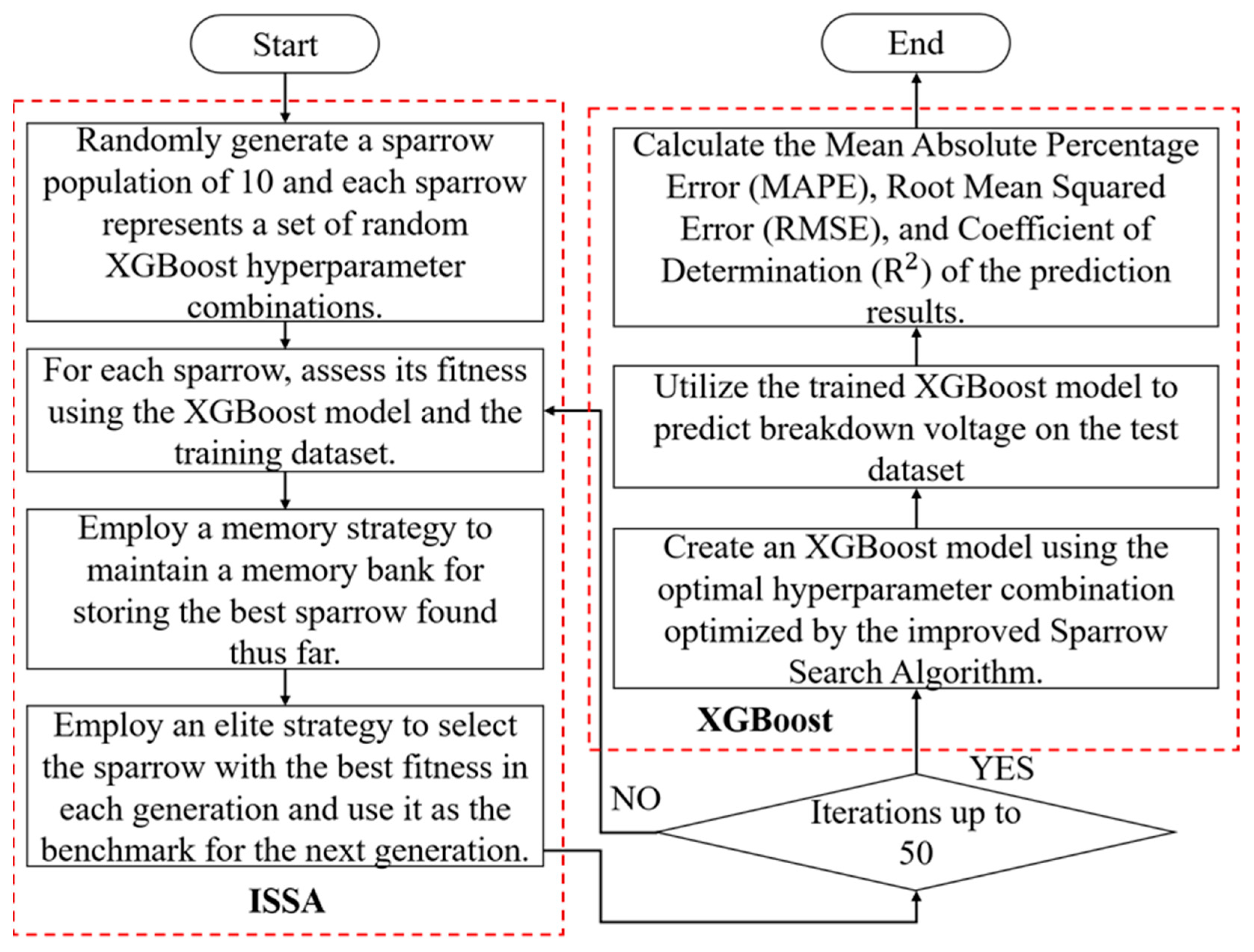
This paper employed the Improved Sparrow Search Algorithm (ISSA) to optimize the hyperparameters of the XGBoost model. The prediction process of the ISSA-XGBoost model is illustrated in Figure 1.
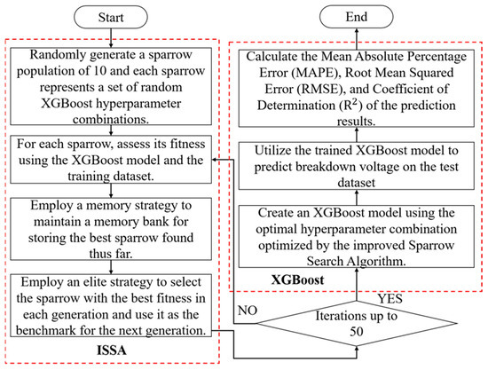
Figure 1.
Prediction process of the ISSA-XGBoot model.
3.1.2. XGBoost
The XGBoost algorithm, proposed by Chen et al. in 2016, is an advancement based on the Gradient Boosting decision tree (GBDT) framework, incorporating both linear scale solvers and tree learning characteristics [26]. The fundamental concept of XGBoost involves integrating multiple decision tree models to make predictions. The model construction process encompasses several critical steps. Specifically, the predictive output of the model is the summation of predictions from all decision trees, and its calculation formula is shown in Formula (1).
where represents the prediction result at the t-th iteration, denotes the weight of the leaf node to which the i-th sample is classified in the k-th tree, is the prediction result from the (t − 1)-th iteration, and pertains to the space of Classification and Regression Trees (CART).
The optimization process of the XGBoost algorithm relies on an objective function composed of a loss function and a regularization term, and the objective function is shown in Formula (2).
where the loss function l is employed to quantify the predictive capability of the model, denotes the number of samples in the training function, and the regularization term Ω serves to govern the structure of the trees.
3.1.3. ISSA
The fundamental principle of the Sparrow Search Algorithm (SSA) is inspired by the division of labor and behavioral patterns observed in sparrow populations during foraging activities, where individuals are categorized into the following three roles: discoverers, followers, and sentinels [27]. However, during the later iterations of the algorithm, rapid convergence among individuals may lead the population to become trapped in local optima. To address this issue, this paper proposed the following two optimization strategies:
- (1)
- Incorporation of an Elite Strategy: By integrating an elite strategy into the SSA, the preservation of superior genetic traits is ensured, preventing the loss of excellent solutions due to random operations [28]. This enhancement boosts the algorithm’s convergence rate and global search capabilities.
- (2)
- Introduction of a Memory Strategy: Within the SSA framework, a memory strategy is employed to record the optimal solutions found during each iteration [29]. These solutions serve as references for subsequent iterations, aiding the algorithm in consistently tracking the optimal solution.
In the Improved Sparrow Search Algorithm (ISSA), the synergistic effects of the elite strategy and the memory strategy optimize the fitness function, which is defined as the sum of the Mean Squared Error (MSE) and the Mean Absolute Percentage Error (MAPE). Furthermore, the number of iterations is increased to 50, thereby enhancing the algorithm’s search capability and the quality of the final solution. Consequently, the position update formula for the individual sparrow in the ISSA is shown in Formula (3).
where t denotes the current iteration number, j = 1, 2, …, d, represents the maximum number of iterations set during initialization, and signifies the j-th dimensional position of the i-th individual in the sparrow population during the t-th iteration. is a random number, and and , respectively, represent the vigilance value and the safety threshold. Q is a random number following the standard normal distribution, and L denotes a 1 × d matrix with all elements equal to 1. is the optimal position of the discoverer recorded by the memory strategy, and is the optimal discoverer selected through the elite strategy. When R2 < ST, it indicates that the discoverer can perform an extensive search for food resources; when R2 ≥ ST, it implies that the discoverer must immediately proceed to a safe area to forage.
The position update formula for followers is shown in Formula (4).
where represents the position of the discoverer and denotes the global worst position during the t-th iteration. A is a 1 × d matrix that satisfies , with each element of the matrix being randomly assigned a value of either 1 or −1. If i > n/2, it indicates that the i-th follower with a lower fitness value must fly to another region to search for food.
The position update formula for sentinels is shown in Formula (5).
where denotes the optimal position within the sparrow population during the t-th iteration; represents a random variable following a normal distribution with a mean of 0 and a variance of 1, which governs the movement of the individual sparrow’s position; and , , and , respectively, indicate the fitness value of the current individual sparrow, the global best fitness value, and the global worst fitness value. The condition implies that the individual is located at the periphery of the population; signifies the necessity for immediate movement towards a safe location; is a constant to prevent division by zero; and is a random number and a parameter variable that controls the movement of the individual sparrow’s position.
3.2. Calculation of Electric Field Eigenvalues
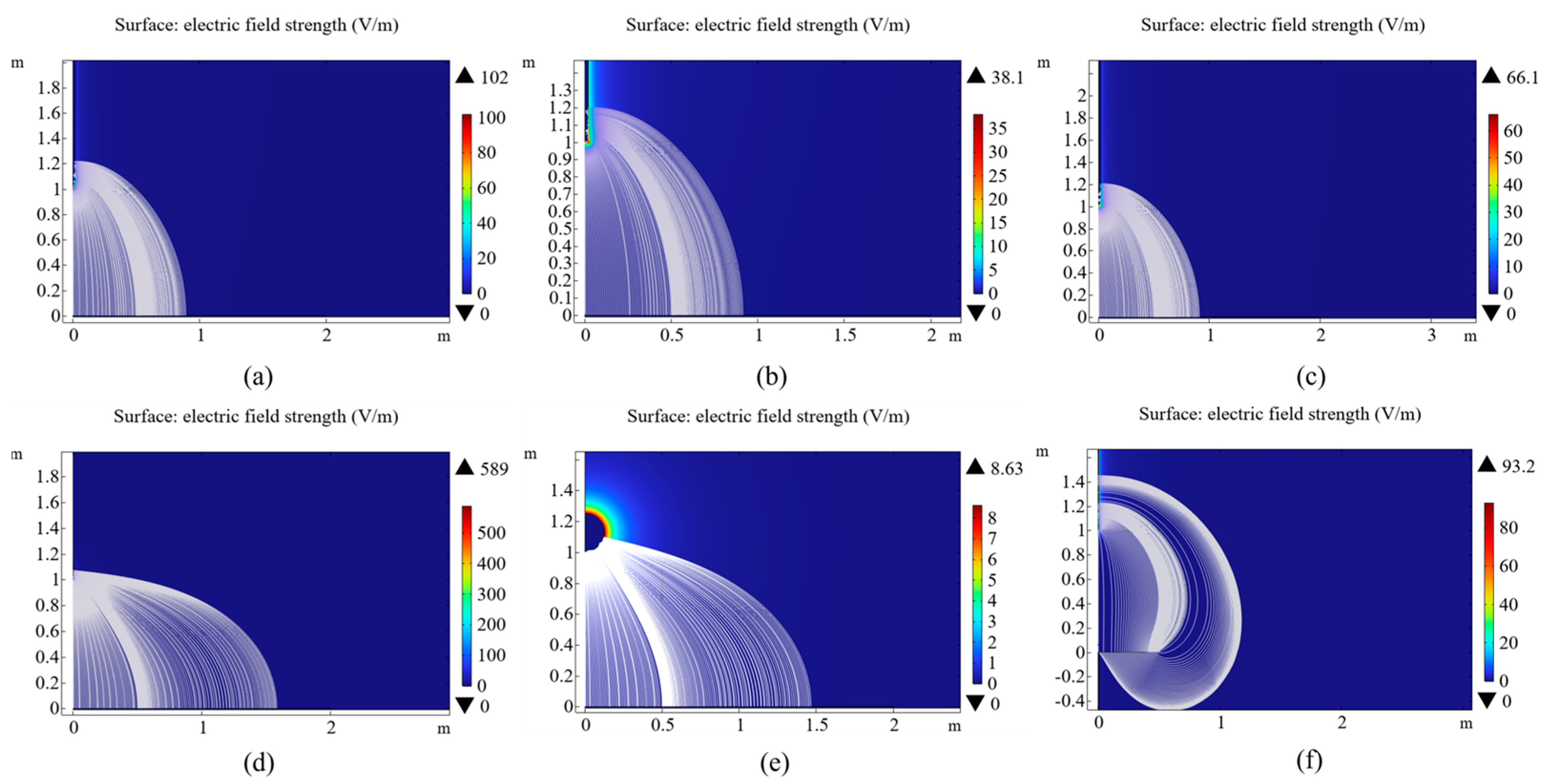
The finite element simulations were performed using COMSOL Multiphysics (version 6.2), a commercial software platform widely adopted for electromagnetic field analysis. Two-dimensional axisymmetric simulation models of rod/sphere–plate and rod–rod long air gap structures were established using finite element simulation software for electrostatic field simulation calculations. Triangular elements were employed for mesh discretization, with finer meshing near the high-voltage electrode, ground electrode, and air gap. A potential of 1 V was uniformly assigned to the high-voltage electrode. A rectangular air gap region, defined by a length equal to half the gap length and a height equal to the gap length, was established between the high-voltage and ground electrodes. Streamlines were set within this rectangular region to calculate the electric field strength in both horizontal and vertical directions. The surface electric field strength distribution for different gap structures is shown in Figure 2, where a-c represented rod–plate gap structures with rod tips of conical, open-ended, and hemispherical shapes, respectively; d represented a rod–plate gap structure with a needle-shaped rod; e represented a sphere–plate gap structure; and f represented a rod–rod gap structure, with both rod tips being open-ended.
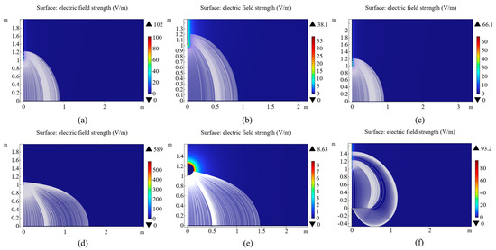
Figure 2.
Surface electric field strength distribution for different gap structures. (a–d) Rod–plate gap; (e) Sphere–plate gap; (f) Rod–rod gap.
The finite element simulation model files were exported to MATLAB software (version R2023a). The calculation process for extracting electric field features is shown in Figure 3, with the specific steps for calculating electric field eigenvalues in MATLAB as follows:
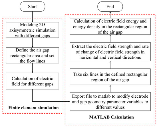
Figure 3.
Calculation procedure for extracting electric field eigenvalues.
- (1)
- The geometric parameters of the electrodes and gaps were modified to variables;
- (2)
- Six lines were sampled in the defined air gap rectangular region according to the sampling rules of 0, 0.05, 0.1, 0.2, 0.4, and 0.8 times the rectangle length. On each line, points were sampled at intervals of 0.01 m, totaling 100 times the line length, to obtain the electric field strength and its rate of change in both horizontal and vertical directions at each point;
- (3)
- A total of 11 sampling points were selected from the above six lines according to the sampling rules of 0, 0.05, 0.1, 0.2, 0.4, and 0.8 times the gap length from the high-voltage electrode, along the shortest path between the electrodes and a path at a 60-degree angle to the shortest path. The electric field strength and its rate of change in both horizontal and vertical directions were extracted for each sampling point;
- (4)
- The defined air gap rectangular region was divided into 36 equal-sized rectangular grid units, with the electric field strength of each grid unit being specified as the electric field strength at the top-left vertex. The electric field energy and energy density of the defined air gap rectangular region were calculated using Formula (6). Since the structure was two-dimensional and axisymmetric, the area of the grid unit was used to replace the volume in Formula (6);
- (5)
- By modifying the geometric parameters of the electrodes and gaps to different values, a 46-dimensional dataset of electric field features could be extracted for each gap structure as input variables for the prediction model.
4. Experiment
4.1. Datasets
Based on the 373 sets of experimental data presented in Section 2.1, an ISSA-XGBoost model for predicting operational impulse breakdown voltage was established. To validate the model’s effectiveness in a rational manner, the dataset was divided into an 8:2 ratio. A total of 298 sets of experimental data were selected as the training set to construct the predictive model, while the remaining 75 sets were utilized as the testing set. The training and testing sets encompass various gap configurations, including rod/sphere–plate and rod–rod structures, with data ranges for gap distance, applied voltage waveform and polarity, and meteorological parameters, as detailed in Table 2 and Table 3, respectively.
Table 2.
Training set data range.
Table 3.
Test set data range.
4.2. Error Metrics
Error analysis is an integral component of model prediction. By calculating error metrics, one can assess the accuracy and applicability of the model, aiding in the optimization of model parameters to achieve superior predictive outcomes. This paper employed three common error metrics, as shown in Formulas (7)–(9).
- (1)
- Mean Absolute Percentage Error (MAPE):
- (2)
- Root Mean Squared Error (RMSE):
- (3)
- Coefficient of Determination (R2):
where n represents the number of predicted samples; Up denotes the discharge voltage value predicted by the model, in kilovolts (kV); Ub is the operational impulse breakdown voltage value obtained from the experiments, in kilovolts (kV); and is the average value of the operational impulse breakdown voltage obtained from the experiments, in kilovolts (kV).
4.3. Results
The training time of the ISSA-XGBoost model proposed in this paper was 0.1931 s, the testing time was 0.0010 s, and the hyperparameter optimization time for XGBoost was 60.2942 s. Upon inputting the test data into the trained ISSA-XGBoost model presented in this paper, the values of MAPE, RMSE, and R2 on the test set were achieved, as shown in Table 4. The MAPE was less than 10%, and R2 was very close to 1. The results indicated that the model proposed in this paper performed exceptionally well, thereby validating the effectiveness of the predictive model.
Table 4.
Prediction results.
A histogram of the relative errors is shown in Figure 4. In Figure 4, the horizontal axis represents the intervals of relative errors, with each interval having a length of 10%. The vertical axis represents the number of samples whose errors fell within the corresponding intervals. As can be seen from Figure 4, among the 75 test samples, 59 samples had relative errors of less than 10%, 8 samples had relative errors between 10% and 20%, and only 8 samples had relative errors greater than 20%. Nearly 80% of the test samples had relative errors of less than 10%, which validated the effectiveness of the model presented in this paper.

Figure 4.
The histogram of the relative errors.
We plotted the regression (R) curve graph showing the predicted values versus the actual values for the test points, as shown in Figure 5. According to Figure 5, both the Pearson’s and R-Square values were very close to 1, indicating a strong linear relationship between the predicted and actual values and excellent model fit.

Figure 5.
The regression (R) curve of the ISSA-XGBoost model.
To ensure the generalizability of the ISSA-XGBoost model to prevent overfitting and provide a more comprehensive assessment of the model’s predictive capabilities, the implementation of k-fold cross-validation was proposed. Specifically, 5-fold cross-validation was chosen due to its balance between computational efficiency and the thoroughness of model evaluation.
The comparison between the results of the ISSA-XGBoost model with and without 5-fold cross-validation is shown in Table 5. Additionally, the MAPE, RMSE, and R2 values obtained from the 5-fold cross-validation were averaged.
Table 5.
The prediction results with and without k = 5 cross-validation.
As shown in Table 5, the comparison of results indicated that, for the ISSA-XGBoost model without 5-fold cross-validation, the MAPE value increased by 1.15%, the RMSE value decreased by 9.02, and the R2 value increased by 0.001 compared to the results with 5-fold cross-validation. The changes in the error metrics were only marginal, with no significant degradation in performance. The results demonstrated that the ISSA-XGBoost model proposed in this paper could effectively prevent overfitting.
4.4. Comparative Study with Traditional Machine Learning Methods
This study conducted a comparative analysis of the proposed ISSA-XGBoost model with several other machine learning models, including Extreme Gradient Boosting (XGBoost), Random Forest Regression (RF) [30], and Gradient Boosting decision trees (GBRT) [31]. Table 6 presents the comparative results of these models on the test set.
Table 6.
Comparative study results with ML.
Based on the results presented in Table 6, it was evident that the ISSA-XGBoost model proposed in this paper demonstrated superior predictive capabilities compared to the traditional machine learning models. The Mean Absolute Percentage Error (MAPE) of the ISSA-XGBoost model was reduced by 1.93% to 4.25%, the Root Mean Squared Error (RMSE) decreased by 25.15 to 42.68, and the Coefficient of Determination (R2) was enhanced by 0.0127 to 0.0067.
We plotted the regression (R) curve graphs of ISSA-XGBoost compared with other traditional machine learning models, as shown in Figure 6. According to Figure 6, the ISSA-XGBoost model had the highest Pearson’s r and R-Square values, closest to 1. This indicated that the model ISSA-XGBoost proposed in this paper had the highest predictive accuracy and reliability, and the best fitting effect.

Figure 6.
The regression (R) curve graphs of different ML. (a) ISSA-XGBoost; (b) XGBoost; (c) RF; (d) GBRT.
To provide a more intuitive comparison of the predictive outcomes of different models, this paper selected 29 test samples under various meteorological conditions, including high temperature, low temperature, high humidity, low humidity, standard atmospheric pressure, and low atmospheric pressure. These samples encompassed both rod/sphere–plate and rod–rod long air gap structures, with data ranges for gap distance, applied voltage waveform and polarity, and meteorological parameters as detailed in Table 7. Figure 7 illustrates the predicted breakdown voltage values for these 29 test samples using the four models, and Table 8 listed the Mean Absolute Percentage Error (MAPE) values for each model.
Table 7.
Information on selected test samples.
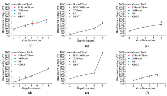
Figure 7.
The comparison results with ML on selected test samples. (a) High temperature; (b) Low temperature; (c) High humidity; (d) Low humidity; (e) Standard atmospheric pressure; (f) Low atmospheric pressure.
Table 8.
MAPE comparison results with ML on selected test samples.
As depicted in Figure 7, the ISSA-XGBoost model exhibited minimal discrepancies between its predicted breakdown voltage values and the actual values across various gap distances. In contrast, other traditional machine learning models, such as XGBoost and Random Forest (RF), demonstrated considerable deviations at certain gap distances. Although Gradient Boosting Regression Trees (GBRT) displayed a relatively stable performance, their predictive accuracy fell short of that achieved by the ISSA-XGBoost model. According to the comparative results of the Mean Absolute Percentage Error (MAPE) presented in Table 8, the ISSA-XGBoost model consistently manifested lower error rates under different environmental conditions. Notably, under high temperature and high humidity conditions, its MAPE values were 3.85% and 2.76%, respectively, which were significantly lower than those of the other models. Despite a relatively weaker performance under low temperature conditions, with a MAPE value of 7.39%, which was slightly higher than that of XGBoost and GBRT, it still remained considerably lower than RF. The average MAPE value of the ISSA-XGBoost model was 4.78%, the lowest among all models, and it achieved a reduction of up to 3.69% compared to the highest value among the other models, thereby highlighting its stability and superiority under various environmental conditions, particularly in extreme meteorological scenarios.
In summary, the breakdown voltage predictions made by the ISSA-XGBoost model were closer to the actual values, and its predictive performance was markedly superior to that of the traditional machine learning models.
5. Discussion
To further evaluate the predictive capability of the ISSA-XGBoost model proposed in this paper, we conducted a comparative study of XGBoost optimized by different algorithms.
The predictive results of the ISSA-XGBoost model were compared with those of XGBoost models optimized by other algorithms, including the Sparrow Search Algorithm, Dung Beetle Optimization Algorithm [32], and Particle Swarm Optimization Algorithm [33]. The selection of SSA, PSO, and DBO for comparative analysis was motivated by their distinct optimization mechanisms and relevance to high-dimensional engineering problems. SSA’s dynamic population roles and adaptability make it ideal for hyperparameter tuning, while PSO serves as a classical benchmark for swarm intelligence. DBO, with its advanced exploration strategies, represents cutting-edge bio-inspired optimization. Table 9 presents the comparative results of error metrics for these models on the test set.
Table 9.
Comparative study results with optimization algorithms.
As indicated in Table 9, the ISSA-XGBoost model significantly outperformed the XGBoost models optimized by the other algorithms. The Mean Absolute Percentage Error (MAPE) of the ISSA-XGBoost model was reduced by up to 1.19%, the Root Mean Squared Error (RMSE) decreased by up to 15.75, and the Coefficient of Determination (R2) was enhanced by up to 0.0039.
We plotted the regression (R) curve graph of ISSA-XGBoost compared with the other optimization algorithms, as shown in Figure 8. According to Figure 8, when compared with the other optimization algorithms, the ISSA-XGBoost model had the highest Pearson’s r and R-Square values, which were closest to 1. The model ISSA-XGBoost proposed in this paper had the best fitting effect and the best predictive ability.
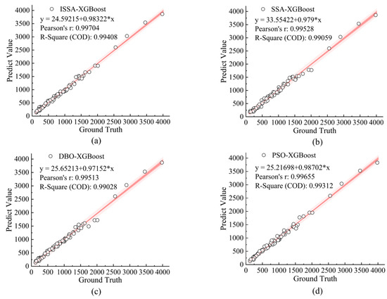
Figure 8.
The regression (R) curve graphs of different optimized algorithms. (a) ISSA-XGBoost; (b) SSA-XGBoost; (c) DBO-XGBoost; (d) PSO-XGBoost.
To provide a more intuitive illustration of the impact of different optimization algorithms on the XGBoost model, this paper selected a subset of test samples identical to those in shown Section 4.4 and plotted a comparative graph of the predicted values from the four models, as shown in Figure 9. The Mean Absolute Percentage Error (MAPE) values for the selected subset of samples for each model are presented in Table 10.
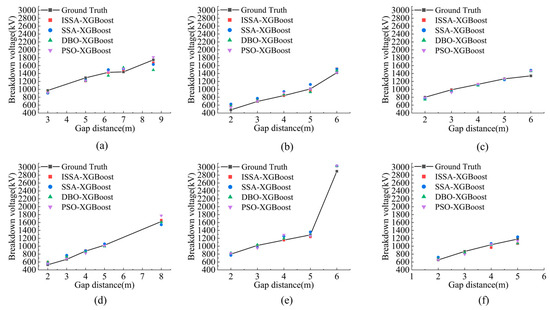
Figure 9.
The comparison results with optimized algorithms on selected test samples. (a) High temperature; (b) Low temperature; (c) High humidity; (d) Low humidity; (e) Standard atmospheric pressure; (f) Low atmospheric pressure.
Table 10.
MAPE comparison results with optimized algorithms on selected test samples.
As illustrated in Figure 9, the ISSA-XGBoost model exhibited minimal deviation between its predicted breakdown voltage values and the actual values across various gap distances. In contrast, SSA-XGBoost and DBO-XGBoost demonstrated considerable predictive errors at certain gap distances, while PSO-XGBoost, although consistently stable in its overall performance, failed to match the predictive accuracy achieved by ISSA-XGBoost. The MAPE values for the different models presented in Table 10 further substantiated this observation. ISSA-XGBoost maintained a consistently low error rate under all environmental conditions, with notably lower MAPE values in high temperature, high humidity, and standard air pressure environments compared to the other models. Although its performance in low air pressure conditions was slightly less impressive, with a MAPE value of 6.40%, which was higher than that of the other three models, its overall average MAPE value stood at 4.78%, the lowest among all models, and it achieved a reduction of up to 2.36% compared to the highest value among the other models, thereby fully demonstrating its stability and superiority under complex environmental conditions.
In summary, the predicted breakdown voltage values from the ISSA-XGBoost model were closer to the actual values, thereby proving that ISSA-XGBoost had significant advantages over XGBoost models optimized by other algorithms.
6. Conclusions
This paper introduced a novel breakdown voltage prediction model, ISSA-XGBoost, which optimized XGBoost using an Improved Sparrow Search Algorithm, resulting in a high level of predictive accuracy. To thoroughly analyze the impact of air gap structure on breakdown voltage, this study constructed two-dimensional axisymmetric simulation models for various long air gap configurations. For each gap structure, 46-dimensional electric field features were extracted.
The model was trained using a training set, and the experimental results on the test set demonstrated that the ISSA-XGBoost model performed well in terms of error metrics, exhibiting good predictive accuracy and stability. Compared to the other traditional machine learning models, the MAPE value of the proposed model was reduced by 1.93–4.25%, the RMSE decreased by 25.15–42.68, and the R2 value was increased by 0.012–0.0067. Furthermore, when compared to the XGBoost models optimized by different algorithms, the ISSA-XGBoost model achieved the highest reduction in MAPE of 1.19%, the highest decrease in RMSE of 15.75, and the highest increase in R2 of 0.0039. These results indicate that the ISSA-XGBoost model significantly outperformed the other traditional machine learning models and XGBoost models optimized by different algorithms in terms of predictive accuracy, especially under extreme meteorological conditions, where the proposed model showed lower error rates and higher predictive accuracy.
The research findings of this paper provide a new perspective for the study of long air gap operational impulse discharge characteristics, aiding in reducing the number of experiments and lowering experimental costs. Although the proposed model achieved significant results, there was still room for improvement in predictive accuracy. Future research will focus on further enhancing the model’s predictive precision.
Author Contributions
Conceptualization, Z.Z., B.S. and S.W.; Methodology, Z.Z., B.S. and S.W.; Software, Z.Z. and S.W.; Validation, Z.Z.; Formal analysis, Z.Z. and S.W.; Data curation, Z.Z.; Writing—original draft, Z.Z.; Writing—review & editing, Z.Z., B.S., S.W., Y.L., D.N. and L.W. All authors have read and agreed to the published version of the manuscript.
Funding
This research received no external funding.
Data Availability Statement
The original contributions presented in this study are included in the article. Further inquiries can be directed to the corresponding author.
Conflicts of Interest
The authors declare no conflicts of interest.
References
- Zhang, Z.; Zhao, J.; Sun, Y.; Jiang, X.; Hu, J. Study on Long Front Time Wave Switching Impulse of Rod-Plane Air Gap. Electr. Power Syst. Res. 2023, 224, 109767. [Google Scholar] [CrossRef]
- Vasudev, N.; Ravi, K.N.; Mujumdar, A.K.; Ratra, M.C. Breakdown Characteristics of Rod-Plane Gap under Salt Fog for AC and DC Voltages. In Proceedings of the Annual Conference on Electrical Insulation and Dielectric Phenomena, Pocono Manor, PA, USA, 17–20 October 1990; pp. 581–586. [Google Scholar]
- Geng, J.; Zhang, H.; Ma, W.; Wang, P.; Liu, Y.; Luo, B.; Liu, L.; Xiao, W.; Zhong, Z. Analysis of Streamer Discharge Characteristics and Voltage Waveform Influencing Factors in Large-Size Sphere-Plate Gap. J. Phys. D Appl. Phys. 2025, 58, 105209. [Google Scholar] [CrossRef]
- Lv, F.; Ding, Y.; Fan, D.; Ding, Y.; Li, Q.; Wang, X.; Yao, X. Characteristics and Altitude Correction of Rod-Rod Long Air Gap Impulse Discharge. In Proceedings of the 2016 IEEE International Conference on High Voltage Engineering and Application (ICHVE), Chengdu, China, 19–22 September 2016; pp. 1–4. [Google Scholar]
- Gallet, G.; Leroy, G.; Lacey, R.; Kromer, I. General Expression for Positive Switching Impulse Strength Valid up to Extra Long Air Gaps. IEEE Trans. Power Appar. Syst. 1975, 94, 1989–1993. [Google Scholar] [CrossRef]
- Mosch, W.; Lemke, E.; Larionov, V.P.; Kolečizky, E.S. An Estimation of the Voltage-Time Characteristic of Long Rod Plane Gaps in Air at Positive Switching Impulse Voltages. In Proceedings of the 13th International Conference on Phenomena in Ionized Gases, Berlin, Germany, 12–17 September 1977; pp. 427–428. [Google Scholar]
- Hutzler, B.; Hutzler-Barre, D. Leader Propagation Model for Predetermination of Switching Surge Flashover Voltage of Large Air Gaps. IEEE Trans. Power Appar. Syst. 1978, PAS-97, 1087–1096. [Google Scholar] [CrossRef]
- Kim, J.-T.; Kim, Y.-S. Prediction of Positive Lightning Impulse Breakdown Voltage Under Sphere-to-Barrier-to-Plane Air Gaps Using Machine Learning. IEEE Access 2024, 12, 120429–120439. [Google Scholar] [CrossRef]
- Qiu, Z.; Ruan, J.; Tang, L.; Xu, W.; Huang, C. Energy Storage Features and Discharge Voltage Prediction of Air Gaps. Trans. China Electrotech. Soc. 2018, 33, 185–194. [Google Scholar] [CrossRef]
- Ruan, J.; Xu, W.; Qiu, Z.; Liao, Y. Breakdown Voltage Prediction of Rod-Plane Gap in Fog Based on Support Vector Machine. High Volt. Eng. 2018, 44, 711–718. [Google Scholar] [CrossRef]
- Qiu, Z.; Zhu, X.; Hou, H.; Zhang, L. Electric Field Distribution Features and Switching Impulse Discharge Voltage Prediction of Long Rod/sphere-plane Gaps. J. Hunan Univ. (Nat. Sci.) 2023, 50, 165–172. [Google Scholar] [CrossRef]
- Qiu, Z.; Ruan, J.; Huang, D.; Pu, Z.; Shu, S. A Prediction Method for Breakdown Voltage of Typical Air Gaps Based on Electric Field Features and Support Vector Machine. IEEE Trans. Dielectr. Electr. Insul. 2015, 22, 2125–2135. [Google Scholar] [CrossRef]
- Qiu, Z.; Ruan, J.; Xu, W.; Huang, C. Energy Storage Features and a Predictive Model for Switching Impulse Flashover Voltages of Long Air Gaps. IEEE Trans. Dielectr. Electr. Insul. 2017, 24, 2703–2711. [Google Scholar] [CrossRef]
- Yang, B.; Lu, Z.; Yao, X.; Shi, W.; Ding, Y. Intelligent Prediction of Positive Switching Impulse Discharge Voltage of Rod-plane Long Gap Based on Regularized IRM-NN. Proc. CSEE 2023, 43, 5683–5693. [Google Scholar] [CrossRef]
- Wang, X. The Comparison of Critical Radius of Rod-Plane Gap at Different Altitudes and Research on Altitude Correction. Master’s Thesis, China Electric Power Research Institute, Beijing, China, 2012. [Google Scholar]
- Ge, X.; Ding, Y.; Yao, X.; Lv, F.; Yang, B. Computation of Breakdown Voltage of Long Rod-Plane Air Gaps in Large Temperature and Humidity Range under Positive Standard Switching Impulse Voltage. Electr. Power Syst. Res. 2020, 187, 106518. [Google Scholar] [CrossRef]
- Wang, Y.; Wen, X.; Lan, L.; An, Y.; Dai, M.; Gu, D.; Li, Z. Breakdown Characteristics of Long Air Gap with Negative Polarity Switching Impulse. IEEE Trans. Dielectr. Electr. Insul. 2014, 21, 603–611. [Google Scholar] [CrossRef]
- Yu, L. Lightning and Switching Impulse Discharge Performance and Voltage Correction of Rod-Plane Air Gaps at Lower Air Pressure in 110 kV System. Master’s Thesis, Chongqing University, Chongqing, China, 2005. [Google Scholar]
- Wang, J. Positive Switching Impulse Flashover Performance and Voltage Correction of Rod-Plane Air Gaps at Lower Atmospheric Pressure. Master’s Thesis, Chongqing University, Chongqing, China, 2007. [Google Scholar]
- Chen, S.; Zhuang, C.; Zeng, R.; Ding, Y.; Su, Z.; Liao, W. Improved Gap Factor of Large Sphere-Plane and Its Application in Calculating Air Gap Clearance in UHVDC Converter Station. High Volt. Eng. 2013, 39, 1360–1366. [Google Scholar] [CrossRef]
- Guo, X.; Ding, Y.; Yao, X.; Fu, Y.; Gao, H. Flashover Characteristics of Sphere-plane Gap and Distance Selection for ±1100kV UHVDC Converter Stations. Proc. CSEE 2020, 40, 3701–3710. [Google Scholar] [CrossRef]
- Geng, J.; Lv, F.; Ding, Y.; Zhao, Y.; Li, P.; Wang, P. Influences of Surface Tips of a Shield Ball on the Discharge Characteristics of a Long Sphere-Plane Air Gap under Positive Switching Impulses. IET Sci. Meas. Technol. 2018, 12, 902–906. [Google Scholar] [CrossRef]
- Arevalo, L.; Wu, D.; Hettiarachchi, P.; Cooray, V.; Lobato, A.; Rahman, M.; Wooi, C.-L. The Leader Propagation Velocity in Long Air Gaps. In Proceedings of the 2018 34th International Conference on Lightning Protection (ICLP), Rzeszow, Poland, 2–7 September 2018; pp. 1–5. [Google Scholar]
- Tu, H.; Fang, Y.; Li, E.; Yang, B.; Fang, J.; Zhang, X. Characterization of Sphere-plane Gap Discharge and Correction Method of Discharge Voltage Under Reduced Air Pressure. High Volt. Eng. 2024, 50, 3580–3588. [Google Scholar] [CrossRef]
- Fang, Y.; Tu, H.; Jia, L.; Li, E.; Liu, L.; Wang, G.; Zhang, X. A Computational Discharge Model for Sphere-Plane Long Air Gap under Switching Impulse Voltage. AIP Adv. 2023, 13, 055127. [Google Scholar] [CrossRef]
- Xiong, X.; Guo, X.; Zeng, P.; Zou, R.; Wang, X. A Short-Term Wind Power Forecast Method via XGBoost Hyper-Parameters Optimization. Front. Energy Res. 2022, 10, 905155. [Google Scholar] [CrossRef]
- Xue, J.; Shen, B. A Novel Swarm Intelligence Optimization Approach: Sparrow Search Algorithm. Syst. Sci. Control Eng. 2020, 8, 22–34. [Google Scholar] [CrossRef]
- Pei, Y. Chaotic Evolution Algorithm with Elite Strategy in Single-Objective and Multi-Objective Optimization. In Proceedings of the 2020 IEEE International Conference on Systems, Man, and Cybernetics (SMC), Toronto, ON, USA, 11–14 October 2020; pp. 579–584. [Google Scholar]
- Gao, H.; Zhao, P.; Yang, Q. A Genetic Algorithm with Memory Function. In Proceedings of the 2022 4th International Academic Exchange Conference on Science and Technology Innovation (IAECST), Guangzhou, China, 9–11 December 2022; pp. 1610–1615. [Google Scholar]
- Dai, Y.; Wang, Y.; Leng, M.; Yang, X.; Zhou, Q. LOWESS Smoothing and Random Forest Based GRU Model: A Short-Term Photovoltaic Power Generation Forecasting Method. Energy 2022, 256, 124661. [Google Scholar] [CrossRef]
- Yang, Z.; Wu, K.; Gu, J. Short-Term Energy Forecasting Based on GBRT and Time Lag Correlation Coefficient. In Proceedings of the 2022 7th International Conference on Information Science, Computer Technology and Transportation, Qingdao, China, 27–29 May 2022; pp. 1–5. [Google Scholar]
- Xue, J.; Shen, B. Dung Beetle Optimizer: A New Meta-Heuristic Algorithm for Global Optimization. J. Supercomput. 2023, 79, 7305–7336. [Google Scholar] [CrossRef]
- Kennedy, J.; Eberhart, R. Particle Swarm Optimization. In Proceedings of the ICNN’95—International Conference on Neural Networks, Perth, WA, Australia, 27 November–1 December 1995; Volume 4, pp. 1942–1948. [Google Scholar]
Disclaimer/Publisher’s Note: The statements, opinions and data contained in all publications are solely those of the individual author(s) and contributor(s) and not of MDPI and/or the editor(s). MDPI and/or the editor(s) disclaim responsibility for any injury to people or property resulting from any ideas, methods, instructions or products referred to in the content. |
© 2025 by the authors. Licensee MDPI, Basel, Switzerland. This article is an open access article distributed under the terms and conditions of the Creative Commons Attribution (CC BY) license (https://creativecommons.org/licenses/by/4.0/).