Study on the Wake Characterization of a Horizontal-Axis Tidal Stream Turbine Utilizing a PIV System in a Large Circulating Water Tunnel

Abstract

In this study, a particle image velocimetry (PIV) system was used in a large circulating water tank to investigate the wake of a horizontal-axis tidal turbine model, focusing on minor blockage effects and scale influence. A wake map of the turbine was constructed based on PIV measurements, using velocity deficit, turbulence intensity (TI), and turbulence kinetic energy (TKE) as key indicators. The results showed that TKE developed later than TI, forming a plateau-like shape. This plateau was considered the decay region, with the transition and far-wake regions located before and after it, respectively. Additionally, the power law exponent of TI decreased from −0.731 in the decay region to −0.765 in the far wake, indicating a steeper decay further downstream. Overall, the wake map of the tidal stream turbine model exhibited similarities to that of a previously reported wind turbine model.

1. Introduction

With growing concerns over environmental pollution and global warming caused by CO₂ emissions, the need for renewable energy has become increasingly urgent, as the world remains heavily reliant on petroleum resources [1,2,3]. Among renewable energy sources, tidal stream energy stands out for its predictability and higher energy density compared to wind energy, allowing for the miniaturization of energy harvesting devices [4,5,6]. Tidal energy can be harnessed through various methods. The barrage-type system utilizes the sea level difference caused by tides by constructing a barrage that stores water at high tide and releases it at low tide to drive a turbine [7,8]. In contrast, the tidal stream method extracts energy from the kinetic energy of tidal currents, using a fluid power turbine to generate electricity [4,9]. While this method requires high tidal flow speeds (2.5–3.2 m/s) [7,10], it does not rely on barrages, making it less restrictive in terms of installation space and minimizing environmental impact. Additionally, since tidal stream turbines are installed underwater, they are less affected by environmental factors such as waves and typhoons [8,9].

The main types of tidal energy harvesting devices studied include horizontal, vertical, and oscillating hydrofoils [7,8,9]. Horizontal and vertical turbines generate energy by rotating a rotor with its axis aligned horizontally or vertically relative to the water flow, respectively. Oscillating foils, inspired by the movement of dolphin and tuna tails [10,11], harness energy by oscillating with the flow of water. Horizontal-axis turbines operate using lift forces, making them more efficient than vertical turbines, which rely on drag forces [12,13]. While various turbine types have been explored, horizontal-axis turbines are the most commercially developed. They operate on the same fundamental principles as wind turbines, allowing existing research on wind energy to be leveraged [14,15]. Through horizontal-axis model experiments, researchers are visualizing the generation and evolution of wakes, including turbine power output and vortex structures. Moreover, studies are actively investigating the mutual interactions between turbines under simulated real-world conditions and different array configurations [16].

One such visualization study analyzed near-wake behavior using particle image velocimetry (PIV). The velocity distribution and flow structure of the near wake were examined using an 800 mm diameter turbine in a towing tank. PIV imaging was performed at full power and at the optimal tip speed ratio, revealing aperiodicity and mutual vortex interactions along the phase-locked, ensemble-averaged, and downstream regions [17]. In a water tunnel experiment with a 500 mm diameter horizontal-axis turbine featuring five blades, PIV visualization was used to analyze turbulent kinetic energy in the near wake [18]. For full wake analysis, PIV imaging was employed to characterize wake behavior by varying the placement of up to four turbines. Adjusting lateral spacing facilitated faster wake recovery, whereas placing turbines too close together impeded recovery. In contrast, longitudinal spacing had no significant effect [19]. Another study used PIV to analyze the full wake of a two-turbine arrangement [20]. Both studies used turbine models with diameters of 0.3 m or less due to facility constraints.

Additionally, several studies have characterized turbine wakes using point velocity measurements based on the Doppler effect instead of PIV. Mycek et al. [21] investigated the interaction of two 700 mm diameter turbines in terms of power and thrust coefficients, analyzing wake profiles and turbulence intensities using laser Doppler velocimetry (LDV). Qian et al. [22] studied the wake characteristics and hydraulic performance of a 1:60 scale horizontal axis tidal stream turbine according to yaw angles (5°, 10°, 15°, 20°, and 30°). The study compared the results of both an experimental approach using acoustic Doppler velocimeters (ADVs) and a numerical approach using the actuator line method (ALM-LES). As the yaw angle increased, the power coefficient decreased, and when the yaw angle was 30°, the power coefficient decreased by 47.1%. The wake pattern was dependent on the yaw angle of the turbine, and the recovery of the wake decreases as the yaw angle increased.

Scaling up turbine size in PIV studies is challenging, as both the PIV device and the turbine must be mounted simultaneously while minimizing blockage effects. Submersible instrumentation is also preferable, adding further complexity. In contrast, computational fluid dynamics (CFD) is free from such scaling limitations, as it utilizes numerical water tanks. Consequently, numerous full wake analysis studies have been conducted using CFD [23,24,25,26]. One study experimentally analyzed wake characteristics using a 700 mm turbine and compared the results with CFD simulations [25]. Similarly, experimental results from a 500 mm turbine were validated against CFD simulations using different turbulence models [23]. In another study, wake effects of a three-bladed horizontal-axis turbine with a 270 mm diameter, placed in a row configuration, were measured using an acoustic Doppler velocimeter (ADV) [27]. Across these studies, turbulence intensity was a key parameter for wake analysis.

On the other hand, it is well known that matching the Reynolds number is the most critical aspect of dynamic similarity in turbine models when minimizing scale effects, which play a significant role in model experiments [17]. This is because the Reynolds number provides the most accurate representation of the flow behavior near turbine blades. If the model size cannot be increased, experiments must be conducted in a flow velocity range where the Reynolds number is independent to satisfy similarity conditions. The scale effect is particularly pronounced in the near wake region [17]. In Nuernberg’s study [19], high rotational speeds were used to satisfy dynamic similarity, and it was reported that this may affect wake development. For the horizontal axis turbine, a Re number of 10⁵ or higher is recommended based on the inflow flow velocity, and a Re number of 5 × 10⁵ or higher is reported to ensure a high level of Re independence [28].

Full wake analysis under conditions that minimize scale and blockage effects has been extensively conducted in wind energy research, where larger facilities are available, and commercialization occurred earlier. Some studies have generated multi-zonal wake maps by analyzing turbulence intensity, turbulent kinetic energy, and other flow characteristics following PIV measurements [29,30]. However, similar studies in the field of tidal stream turbines remain limited due to the constraints mentioned above.

As previously introduced, studies on wake visualization, output, vortex shape, turbine arrays, and interactions between turbines provide essential insights for the deployment of power plants aimed at energy harvesting through tidal turbines. To assess the overall energy harvest, it is crucial to understand the individual efficiency of the turbines and the impact of the turbine wake on nearby turbines. A visual representation of the flow information in the full wake, including near wake and far wake, in the form of a wake map can serve as a criterion for turbine array configuration. To obtain more reliable wake information, it is necessary to minimize scale effects and block effects while adhering to Reynolds’ criterion. Additionally, for generating visualization images, it is preferable to analyze the flow area using particle image velocimetry (PIV) rather than relying on interpolation through point measurements.

In this study, we aim to construct a PIV system capable of precise flow analysis in a large circulating water tunnel, minimizing the scale and blockage effects. Using this system, we seek to generate a full wake map and analyze wake characteristics based on velocity deficit, turbulence intensity, and turbulent kinetic energy.

2. Materials and Methods

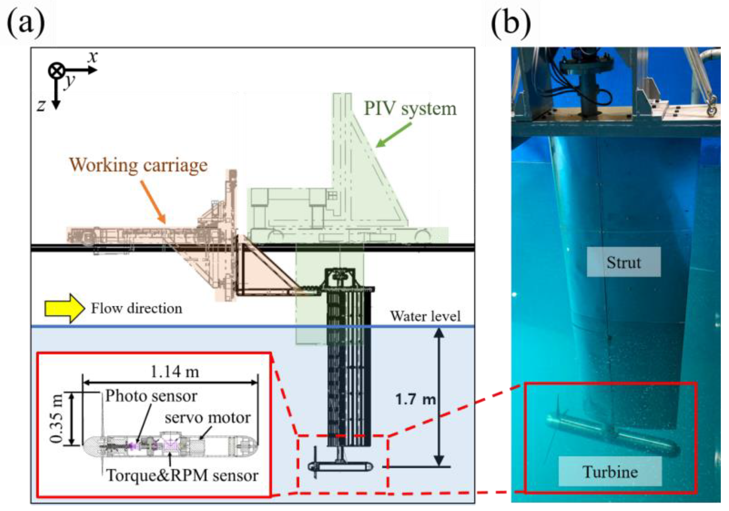
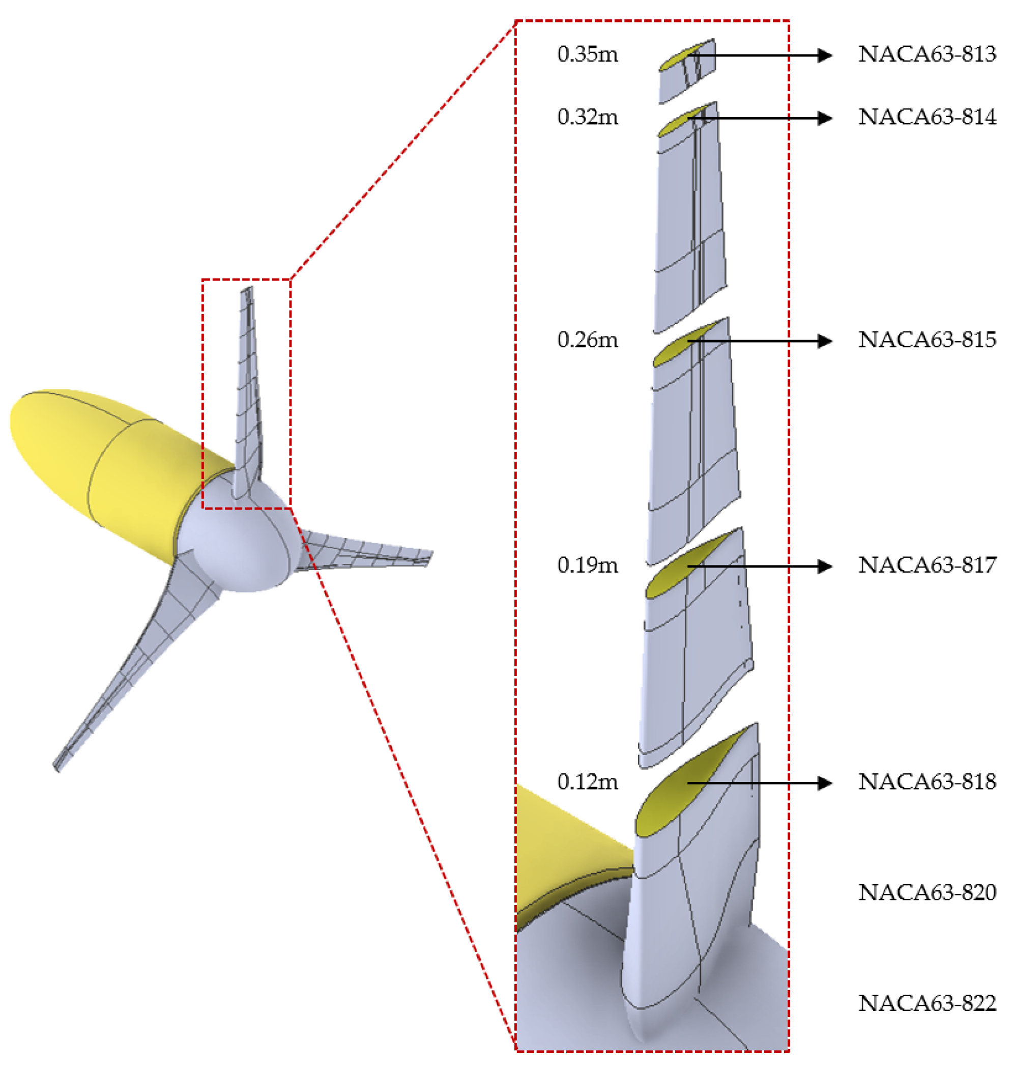
2.1. Turbine Apparatus

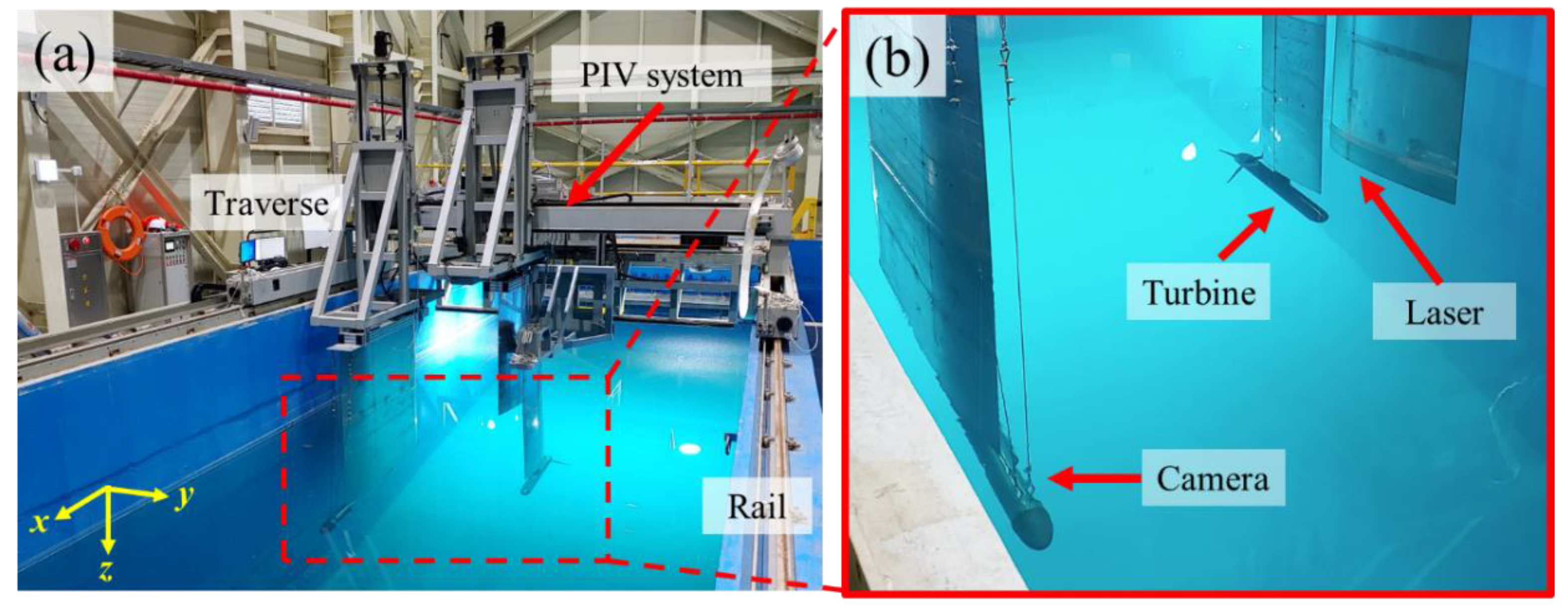
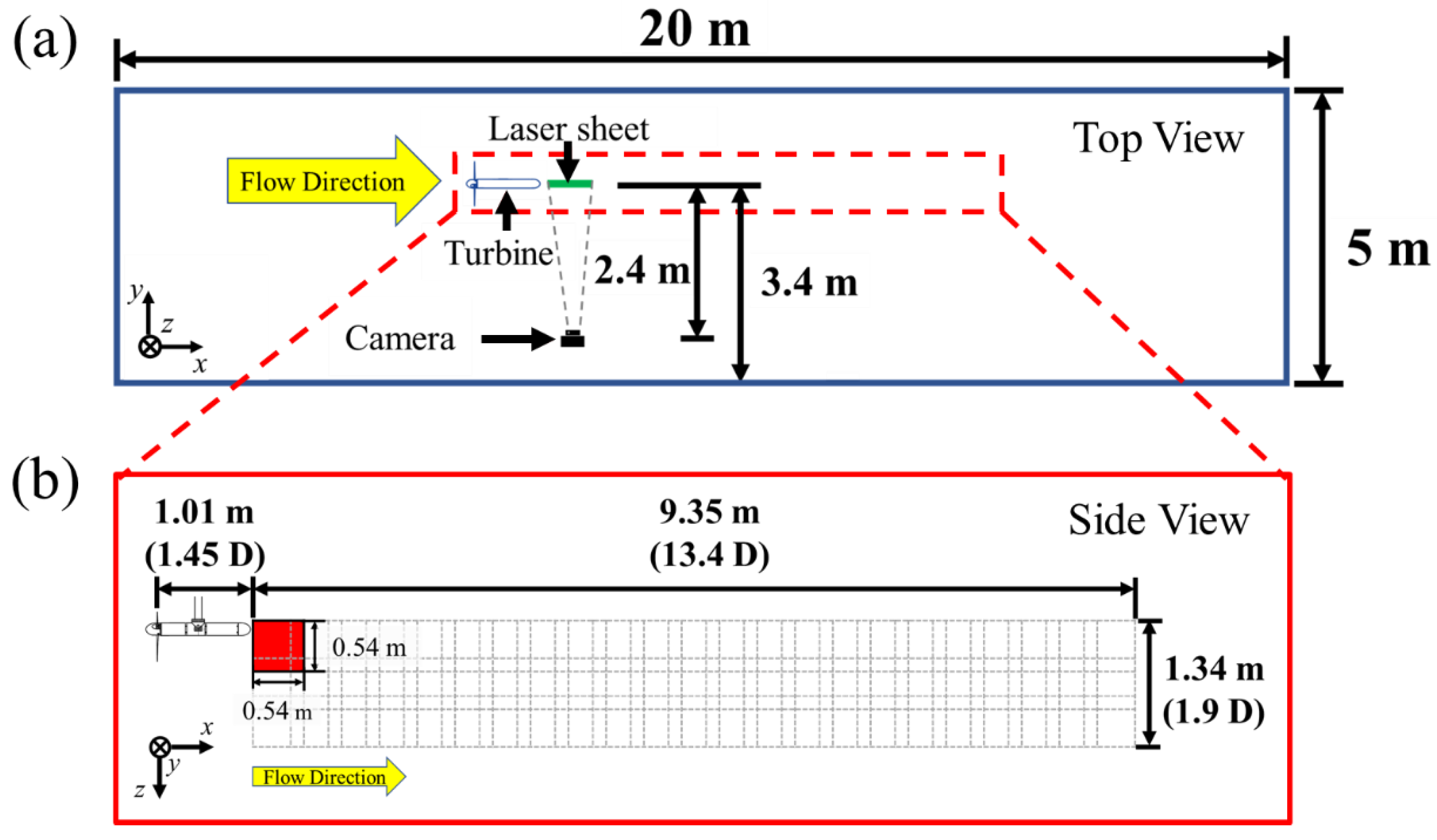
The experiments were carried out in a large circulating water tunnel (CWT) at the Marine Robotics Demonstration Center in Pohang City, South Korea. This large-scale CWT is 20 m long, 5 m wide, and 5 m deep, and the maximum flow velocity can be set to 1.76 m/s. The shape of CWT is horizontally opposed, and a honeycomb structure is installed inside to prevent flow delamination and create a uniform flow field in the test section, as well as a guide vain to change the rotation and pressure of the flow velocity.

Figure 1a is a schematic diagram of the turbine and equipment arrangement, and Figure 1b is an actual photograph of the turbine and strut structure. The working carriage and the PIV system can be positioned independently and simultaneously on the rails of CWT, and the experimental position and the PIV acquisition position can be adjusted by changing the position of each other. The entire working carriage can be moved along the rails in the x direction, and the turbine and strut structure are attached to a traverse that moves in the y and z axes to facilitate positioning of the turbine in CWT. The PIV system will be described later in the following section.

The strut has an outer diameter of 76.3 mm, a thickness of 7.0 mm, and a length of 3.27 m, with the turbine’s nacelle attached at the end. The strut is covered with a NACA 0022 type sheath that is not in direct contact with the strut, which is designed to minimize the loads imposed by the fluid directly on the strut in addition to the loads imposed on the turbine body.

The nacelle is 0.138 m in diameter and 1.14 m long, and it is equipped with a 750 W servo motor (SGM7J-08AFD21, YASKAWA), a torque-RPM sensor (T21WN, HBM), and a photo sensor (PM-L25, Panasonic) inside (Figure 1 Inset). Since the sensors and motor are submerged in water, a mechanical seal was used to seal the rotating shaft. Mechanical seals were chosen to increase water-tightness in consideration of long-term operation. The motion control of the rotation speed and torque of the blade shaft is performed by a servo motor inside the nacelle and does not use gears for power transmission, so the torque-RPM value was measured without power loss due to the gears. A photo sensor was used for PIV acquisition at the same blade position (phase averaging), which will be explained further in the following section.

The turbine used in the experiments has a diameter of 0.7 m and consists of three blades. The blades are made of aluminum AL6061 with good machinability and corrosion resistance and are anodized. The geometry changes from root to tip from NACA63 822 to NACA63-813 according to the cross-sectional station information of the blades as shown in Figure 2, and these geometries were obtained by blade element momentum theory (BEMT) and parametric analysis.

In order to evaluate the performance of the turbine with the blade with the corresponding geometry, the power coefficient (C_p) is derived from the tip speed ratio (TSR) as follows:

TSR = rΩ/U

(1)

where r is radius of turbine, Ω is angular velocity (rad/s), and U in incoming velocity, and

C_p = ΩT/(0.5ρU³ πr²)

(2)

where T is the torque and ρ is the density of water (at 18 °C, the density of water is 998.60 kg/m³).

Tidal stream turbine operation is dependent on the inertial force and turbulence of the fluid, and many studies have reported that the upper bound through Reynolds number is more appropriate in such an environment [28]. Therefore, in this study, the performance of the turbine was tested in the range of 5 × 10⁵ where Re independence is guaranteed based on the Reynolds number as shown in the equation below.

Re = (U₀ c)/ν

(3)

Here, the flow velocity is U₀, the chord length is c, and the kinematic viscosity coefficient is ν [31]. The flow velocity at this time is 1.0 m/s and was measured by PIV imaging without the turbine. PIV flow measurement will be described in more detail later.

For the turbine performance experiments, the center of the turbine was placed at a depth of 1.7 m of the CWT. A servo motor inside the turbine was used to control the rotation speed of the turbine by applying torque in the direction opposite to the direction of rotation of the shaft rotated by the flow, and the resulting efficiency changes were compared.

2.2. PIV Apparatus

As shown in Figure 3, the PIV system is shaped to allow the camera and laser to be submerged in water, and the submerged area is covered with a streamlined cover to minimize shaking due to flow. Like the working carriage, the entire PIV system can be moved along rails in the x direction. The camera and laser are attached to individual traverses and can be positioned independently in the y and z directions. The CCD camera has a resolution of 25 MP and a shooting speed of 180 fps (Model 630098, TSI Inc., Shoreview, MN, USA) and is equipped with a 532 nm filter to attenuate light sources outside the laser wavelength and a zoom lens (NIKKOR 105 mm, Nikon Inc., Tokyo, Japan) for easy adjustment of the angle of view underwater. The laser is an Nd:YAG type with an output power of 200 mJ and a wavelength of 532 nm (Quantel, Evergreen Inc., Taoyuan, Taiwan), and the dedicated cylindrical and spherical lenses allow for the irradiation of laser sheets with a thickness ranging from 2 to 5 mm.

Before measuring the flow of the turbine, PIV measurements were first made without the turbine to understand the flow characteristics in the CWT. Then, for the PIV flow measurement, the turbine was controlled under the following conditions. A servo motor was controlled to apply a torque to the shaft in the direction opposite to the direction of rotation to control a targeted TSR of the turbine. The turbine efficiency is maximized when a torque of 3.37 N-m is applied at 1.0 m/s (TSR 5.95), but there is a problem of overloading the motor when operating for a long time at such a torque, so PIV imaging was performed at a larger TSR of 7.17 for stable turbine operation. The photo sensor was used to capture the blade position at 6 o’clock, and 128 images were taken for each section and phase averaged.

The tracer particles used for PIV (1101-1000, INTECH SYSTEMS, Ahmedabad, India) were 100 μm in size and polyamide with a density of 1.1 g/cm³. The experimental flow velocity was 1.0 m/s, the same as the performance test of the turbine. The location of the turbine was at a depth of 1.7 m and 3.4 m away from the wall as depicted in Figure 4. Due to the interference of the PIV system with the installed part of the turbine, PIV measurements were performed from a position corresponding to the end of the turbine body (nacelle) (1.45 D distance from the blades). The laser sheet was irradiated in the same plane as the turbine center and parallel to the water flow direction, and the laser pulse time interval was 5000 μs. The horizontal distance between the camera and the laser sheet was 2.4 m, and the field of view at this position is 0.54 m × 0.54 m, with a spatial resolution of 105.80 × 105.80 μm/pixel. The camera of the PIV system was moved by 0.4 m in the x and z directions to ensure that the overlap between the FoV sections was 0.14 m in the x and z directions, and a total of 23 sections in the x direction and 3 sections in the z direction were taken, resulting in a total measurement area of 9.35 m (13.4 D) in the x direction and 1.34 m (1.9 D) in the z direction.

PIV images were acquired and processed using Insight 4G (11.1.0.7, TSI, Inc.) software. The Recursive Nyquist Grid engine was used to generate a 50% overlap grid, and the spots were conditioned with a Gaussian Mask, with starting spot dimensions of 256 × 256 pixel and final spot dimensions of 128 × 128 pixel. The correlation map was derived using a fast Fourier transform (FFT) correlator.

3. Results

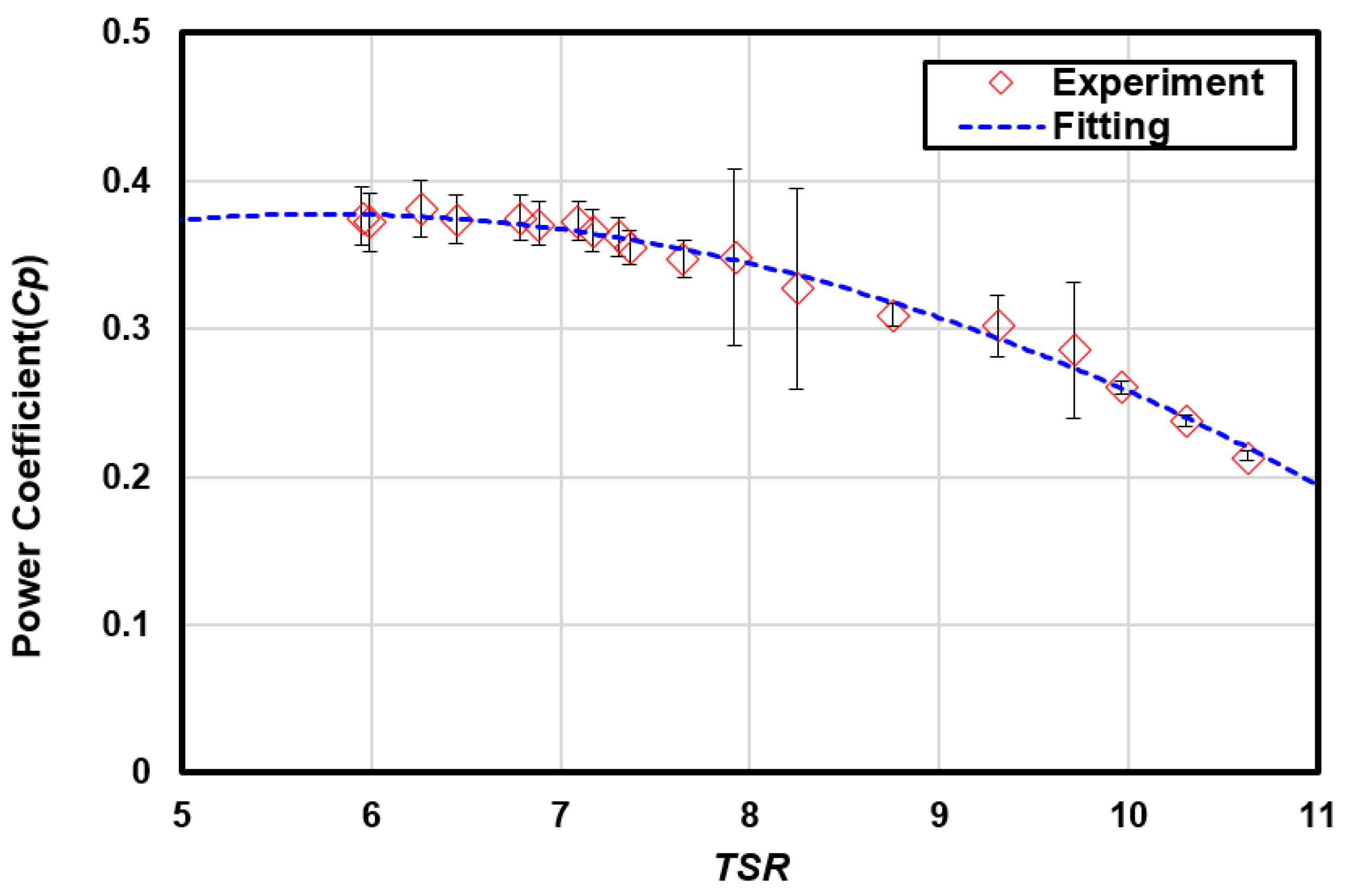
3.1. Power Performance of the Turbine

The experimental Cp curve for the turbine model is shown in Figure 5. In the case of the experiment, the counter-loading of the motor was imposed, so at lower TSRs, reverse rotation occurred and could not be measured. Also, the effect of the mechanical seal was included because it was used for a long-time underwater operation, as described earlier. As a result, a maximum Cp of 38%, which was smaller than the value designed by BEMT due to the counter-loading by the motor control and the seal use, was obtained at a TSR of 5.95.

3.2. PIV Result

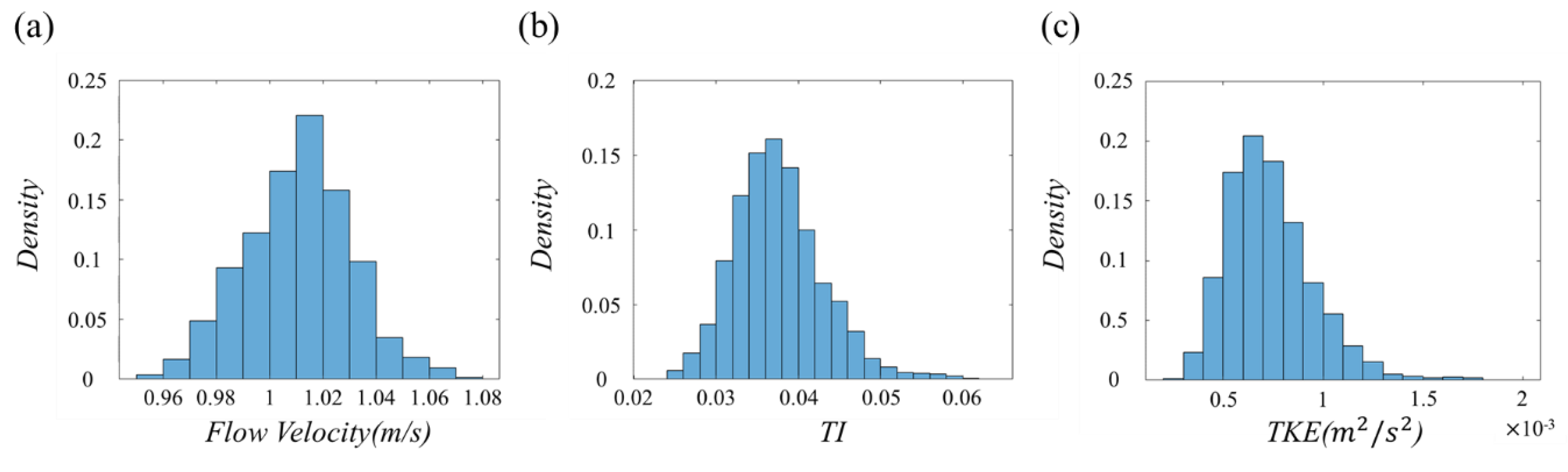
3.2.1. Flow and Turbulence Distributions Without the Turbine

Prior to the PIV acquisition downstream of the turbine, the flow conditions over the PIV measurement area were verified. The average flow velocity (U), turbulence intensity (TI), and turbulent kinetic energy (TKE) were derived from the 64 PIV data for each measurement section in the absence of the turbine, and the flow velocity value for the overlap section was calculated using the arithmetic mean and then was depicted in Figure 6. Each result is shown in a contour plot in Figure 6, and the contour level is represented by the same range as the flow result of the turbine through the PIV. The flow velocity (U) was derived from the sum of the x-direction flow velocity (u), and the z-direction flow velocity (w) was obtained through the PIV measurement and is shown in the equation below.

$$\mathrm{U}=\sqrt{{\mathrm{u}}^2+{\mathrm{w}}^2}$$

(4)

The flow velocity under a free flow (U), obtained by averaging the flow velocity over the measurement area, is 1.0 ± 0.02 m/s. The turbulence intensity is defined as the standard deviation of the flow velocity divided by the flow velocity; it is given by the equation below.

$$\mathrm{T}\mathrm{I}={\displaystyle \frac{\sqrt{\overline{{\left({\mathrm{u}}^{\prime }\right)}^2}+\overline{{\left({\mathrm{w}}^{\prime }\right)}^2}}}{\mathrm{U}}}$$

(5)

where u′ is the standard deviation of the flow velocity (u) in the x-direction and w′ is the standard deviation of the flow velocity (w) in the z-direction. The average turbulence intensity across the measurement area was 0.038 ± 0.005.

The turbulent kinetic energy represents the kinetic energy of the flow due to turbulence and is the sum of the variance of the velocity components divided by half.

$$\mathrm{T}\mathrm{K}\mathrm{E}={\displaystyle \frac{1}{2}}\left(\overline{{\left({\mathrm{u}}^{\prime }\right)}^2}+\overline{{\left({\mathrm{w}}^{\prime }\right)}^2}\right)$$

(6)

The average turbulent kinetic energy of the entire measurement area was 0.0007 ± 0.0002 m²/s². Although Figure 6 shows a somewhat grid-like pattern due to the math processing in the overlap section, the flow distribution was relatively uniform with no unusual flow such as boundary layer flow or surface flow effects in either the vertical or horizontal direction. Figure 7 represents the PDF (probability density function) of the (a) flow velocity, (b) TI, and (c) TKE without a turbine. Each graph shows a uniform distribution of a bell-shape that shows high density at the value near the average value. A PDF close to a Gaussian distribution supports the uniformity of the contour image.

The turbulence intensity and turbulence kinetic energy without turbine were very low compared to the average turbulence intensity and turbulence kinetic energy within the turbine wake area, 0.17 and 0.008 m²/s² respectively, which will be described later. Therefore, it was considered that the incoming flow had little influence on the measurement of turbulence in the turbine wake. Although the turbine was not located in the center of the CWT due to equipment limitations and to ensure a large FoV, stable flow conditions were achieved at this location. This can be attributed to the fact that the experiments were conducted in a large CWT and were taken in an area sufficiently distant from the nearest CWT wall, 1.6 m (2.3 D), and 3.3 m (4.7 D) from the bottom of the CWT.

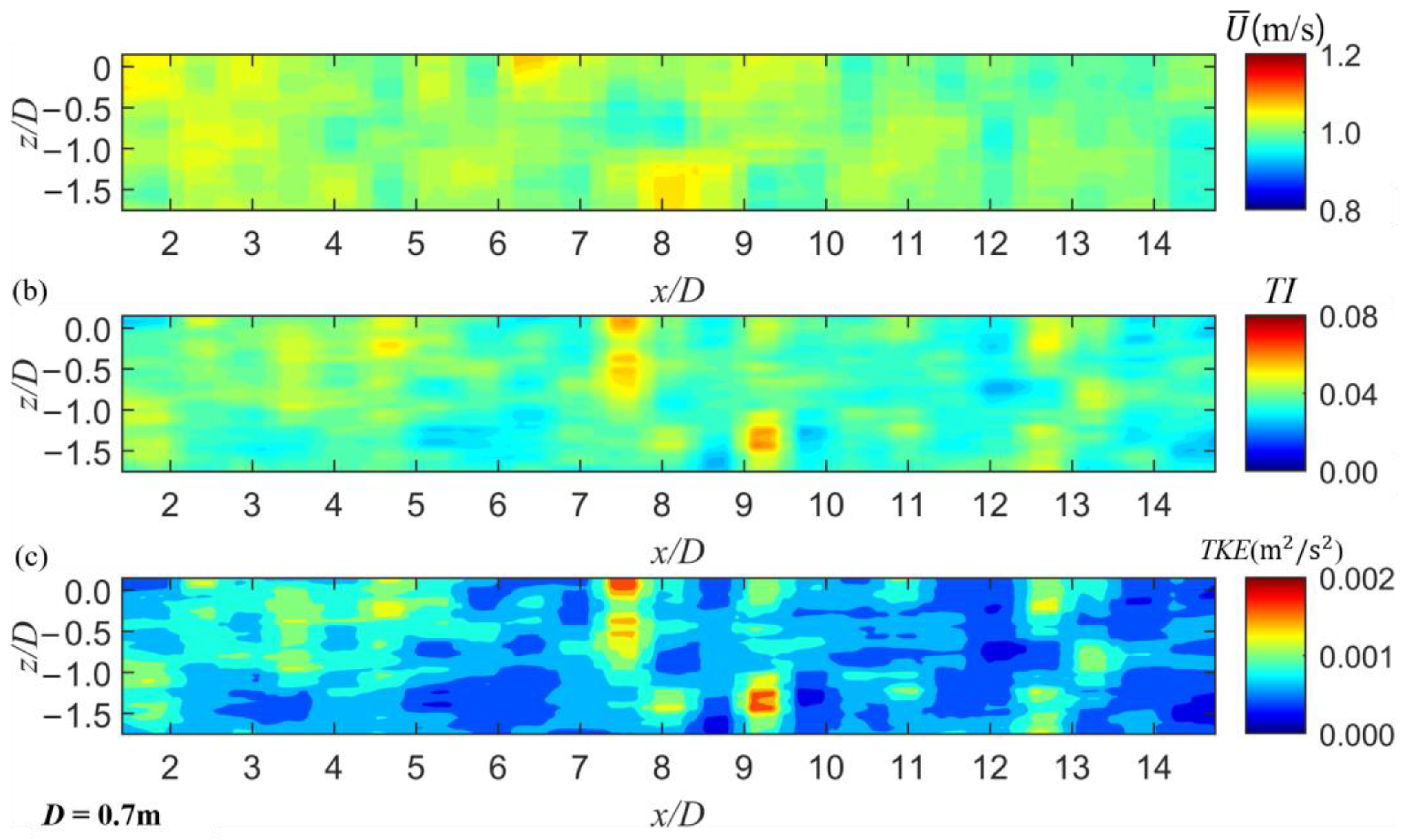
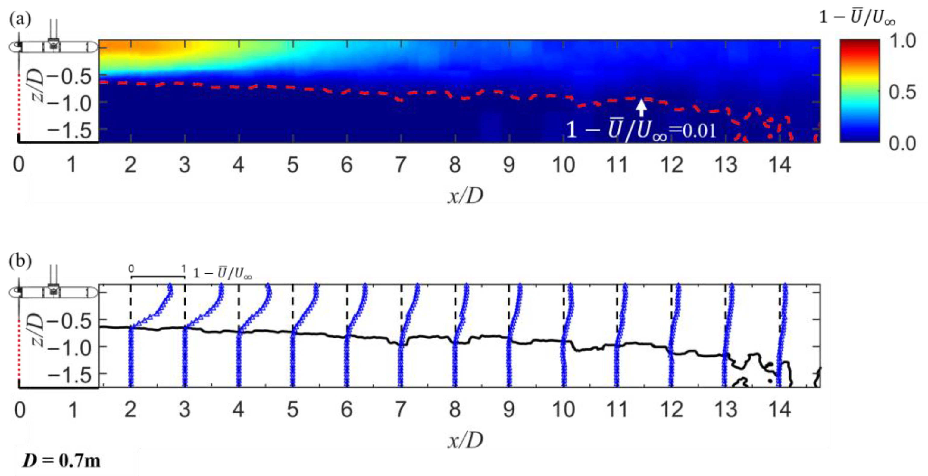
3.2.2. Flow Distribution with the Turbine

The flow velocity distribution downstream of the turbine when TSR was 7.17 is shown in Figure 8 in the form of the velocity deficit in the form of the below expression. This was the difference between the flow velocity in the wake and the flow velocity in free flow ($\overline{U}-U_{\mathrm{\infty }}$), normalized to the flow velocity in free flow ($U_{\mathrm{\infty }}$), indicating how much the flow velocity had decreased relative to free flow.

$$\mathrm{Velocity} \mathrm{deficit}={\displaystyle \frac{\overline{U}-U_{\infty }}{U_{\infty }}}=1-{\displaystyle \frac{\overline{U}}{U_{\infty }}}$$

(7)

Downstream of the turbine, the flow velocity was significantly reduced compared to the free flow, and the velocity deficit immediately behind the nacelle was found to be 0.73. At 1.45 x/D, which corresponded to the start of the measurement region, the boundary of the wake with reduced velocity compared to free flow can be seen to start at z/D = −0.61, which was near the horizontal position of the turbine blades. Since the boundary of the wake was shown to expand as we proceeded in the flow direction from the blade position [32,33,34], it is concluded that the boundary of the wake existed further downstream than z/D = −0.5, which corresponded to the horizontal position of the turbine blade tip. The boundary of this wake was found to be divided by the contour line 1 − $\overline{U}/U_{\mathrm{\infty }}$ = 0.01, and was advanced 13 x/D. It can be seen that the velocity deficit changed parabolically from the top of the boundary to the bottom of the centerline of turbine, recognizing that 1 − $\overline{U}/U_{\mathrm{\infty }}$ = 0.01 is an appropriate boundary for the flow. The decreased velocity gradually recovered as the flow proceeded downstream.

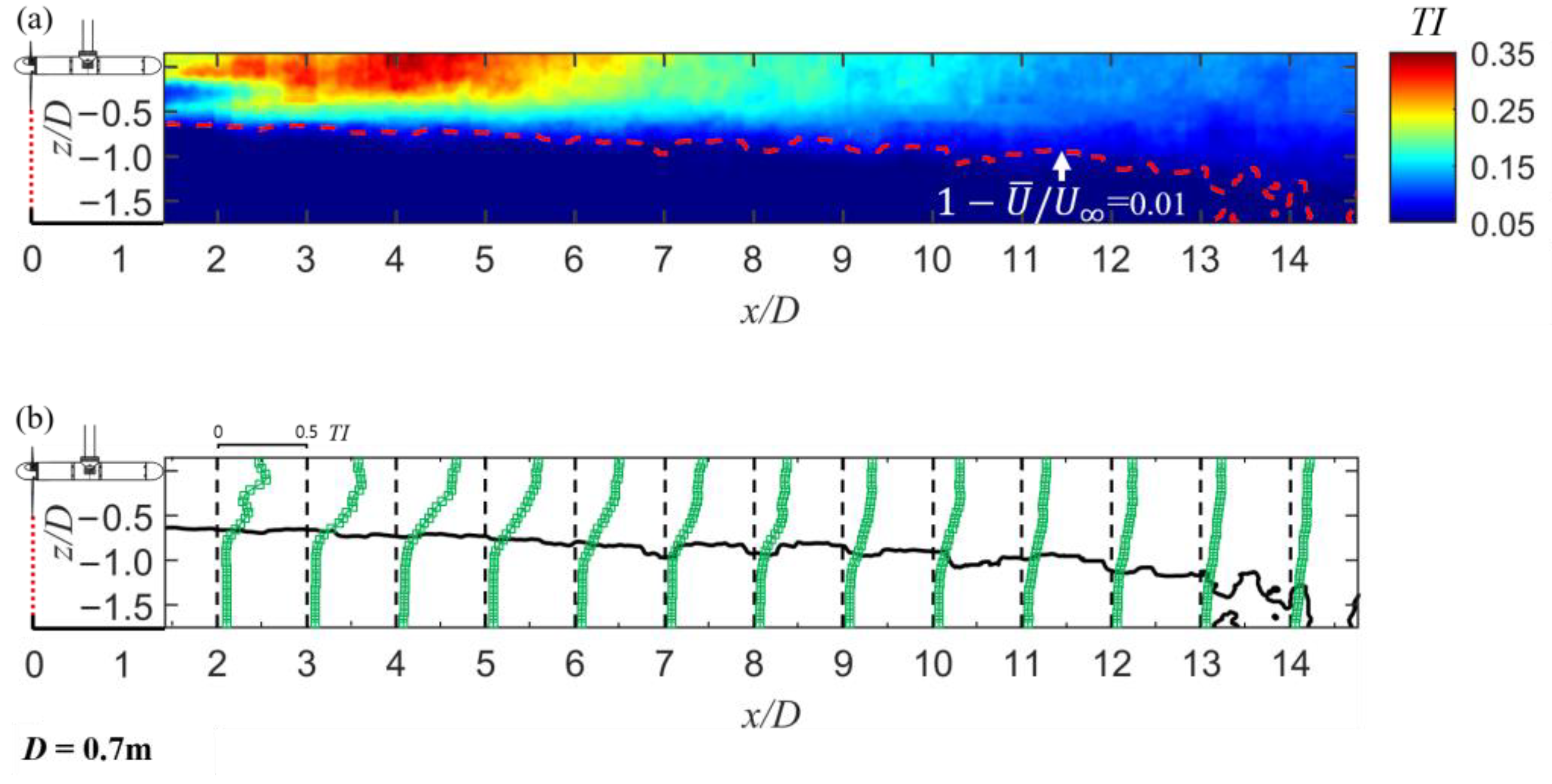
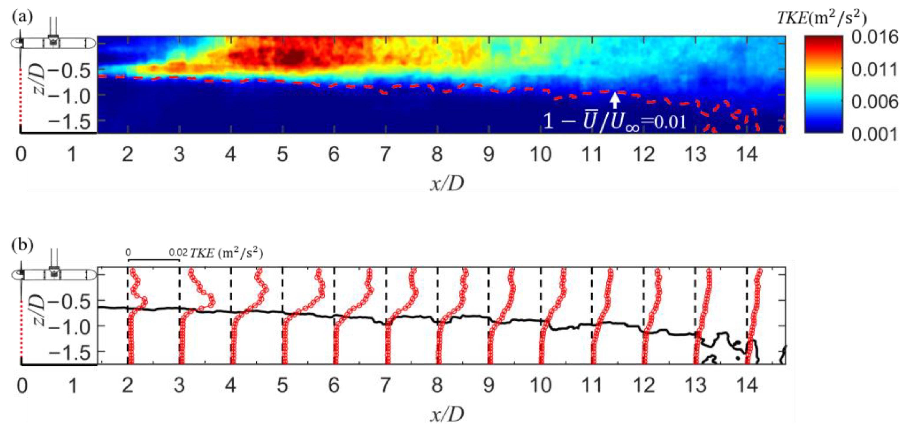
3.2.3. Turbulence Distribution with the Turbine

The turbulence intensity in the wake began to originate from the blade tip and the root tip, and the width was not significant at 1.45 x/D, which corresponded to the starting position of the measurement area, but as the x direction increased, the turbulence intensity from the root tip increased and the width increased. A high level of turbulence intensity was observed around 4 x/D, which is presumed to be caused by the merger of two turbulences generated at the blade tip and root. The velocity deficit distribution in the wake of the turbine showed the highest velocity deficit at 1.45 x/D, behind the nacelle, and the flow velocity tended to recover as the wake progressed in the x direction, but the turbulence intensity increased until the 4 x/D, after which the turbulence intensity decreased, but the influence of the wake remained until the end of the measurement region at 14 x/D. Similar to the velocity deficit distribution, the turbulence intensity distribution also showed a different distribution shape based on the contour line 1 − $\overline{U}/U_{\mathrm{\infty }}$ = 0.01. As shown in Figure 9b, it can be seen that the turbulence intensity increased parabolically above the boundary. This confirms that the contour line 1 − $\overline{U}/U_{\mathrm{\infty }}$ = 0.01 is a valid boundary not only for velocity deficit but also for turbulence intensity.

Unlike turbulence intensity, which indicates the amount of turbulence relative to flow velocity, turbulence kinetic energy directly shows the turbulence energy in the wake. As shown in Figure 10, the TKE primarily originated at the tip of the blade, and there was also TKE at the root of the blade, albeit to a lesser extent. This shows that the turbulent energy in the wake was dominantly generated at the tip of the blade. The TKE generated at the blade tip increased in value in the x direction and developed in the z+ direction. Due to this developing aspect of the TKE, there was a region of wake core with low TKE distributed behind the nacelle surrounded by relatively high TKE flow. This suggests that higher levels of TKE were generated at locations further away from the turbine than near the blades where turbulence was generated.

The turbulence intensity represents the fluctuation of the flow velocity relative to the flow velocity, so the fluctuation is low directly behind the turbine, but the flow velocity is also low, resulting in a relatively high value. However, in reality, the area directly behind the turbine was found to have a low TKE due to the low fluctuation in flow velocity. The TKE was highest at about 5 x/D and decreased gradually thereafter, but there was still some downstream TKE after 14 x/D. The TKE distribution also showed that the boundary of the wake was divided by the 1 − $\overline{U}/U_{\mathrm{\infty }}$ = 0.01 contour line, which suggests that 1 − $\overline{U}/U_{\mathrm{\infty }}$ = 0.01 is a good choice for the wake boundary.

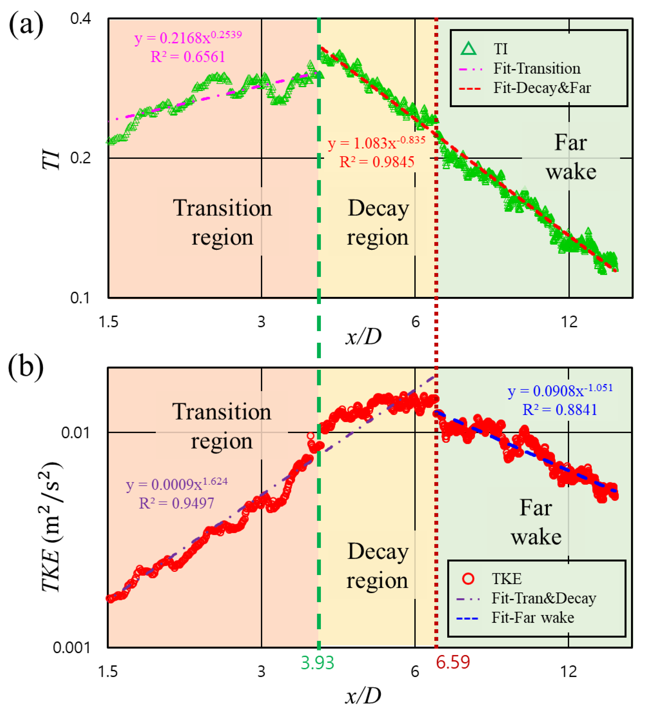
3.2.4. Decay Zone in Wake Map

From the previous distribution plots, we can see that the velocity deficit started at 0.45 x/D, the TI started to decrease at 5 x/D, and the TKE started to decrease at 6 x/D. TI and TKE were graphed separately for the increasing and decreasing parts, as shown in Figure 11. As shown in the figure, we can see that the level of increase and decrease was greater for TKE, which means that the two indicators of turbulence had different maximum points and different rates of decrease. The question then becomes, what value of the metric can determine the point of decay in turbulence level in the wake?

An answer is that for wind power, Neunaber et al. [29] determined this as the variance of the turbulence intensity and flow velocity at the centerline with respect to the rotor position. Here, the variance represents the square of the standard deviation of the flow velocity and is twice the TKE. Neunaber et al. [29] showed that the region around the maximum value of the variance is similar to a plateau, and two inflection points were derived around the maximum value of the variance to define the downstream position where the decay of the wake begins. Namely, the area between the two inflection points was defined as the plateau and the corresponding area as the decay region. Subsequently, the region after the second inflection point corresponded to far wake. The difference in flow patterns in the decay region and far wake can be distinguished not only in TKE but also in TI. To show differences depending on the region, the power law (TI∝α∙(x/D)^β), which represents the self-similarity of turbulence, was used. The equation was applied to TI data in the decay region and far wake, respectively, and found that the slope of the curve changed. A similar plateau region was also found in the TKE curve of this study, and the curvature change around the maximum value is shown as a dotted line in Figure 12.

The first inflection of the TKE curve was identified at 3.93 x/D, and the second inflection at 6.59 x/D. Below the first inflection point, from 1.45 x/D to 3.93 x/D, the TI increased up to 3.93 x/D, where it had a maximum value, and it can be considered as a transition region because it fulfills the condition that the TI builds up while the flow deficit mainly increases to a high level, as presented in Figure 13 of Neunaber et al. [29]. The region between 3.93D and 6.59D can be considered as a decay region because it satisfies the condition that the flow velocity recovers, but the TI decreased as described in Figure 13 of Neunaber et al. [29]. After 6.59D, when the TKE curve passed the second inflection point, the flow velocity kept recovering, and the TI decreased as well, so it can be considered as a far wake region where turbulence dissipates. Following the same trend in the case of Neunaber et al. [29], the βs of the power law of the turbulence intensity in the decay region and far wake were different, −0.731 and −0.765, respectively, meaning that the turbulence intensity decreased faster in the far wake.

Next, the velocity deficit, TI, and TKE curves were plotted in Figure 13 for a full wake map consisting of the above three regions. The closest experimental results under similar conditions were from a previous study [21] where laser Doppler velocimetry (LDV) measurements were taken in a CWT experiment with a 70 cm diameter three-blade horizontal axis turbine. It was found in condition of the TI of 3% without turbine that the velocity with turbine was significantly reduced within the range of 3~4 x/D; the TI was high within the range of 4~7 x/D; and the Reynold shear stress, $\left|\overline{u\prime v\prime }\right|$, which is a metric similar to TKE, was high at range of 5~8 x/D, which was somewhat behind from the that of TI; thus, the map was presented at a TSR of 3.67, which is somewhat smaller than the present study, but the trend was similar to the results of this study.

When considering array deployment, it is most recommended to locate the downstream turbine after 10 x/D, where all three metrics drop to low levels, but for dense deployment, it is possible to consider between 6.59 x/D and 10 x/D, where turbulence levels decrease.

4. Conclusions

In this study, a particle image velocimetry (PIV) system was deployed in a large circulating water tank to measure the wake of a three-blade horizontal axis tidal turbine with a 70 cm diameter up to 15D to minimize scale and blockage effects and for precise flow analysis.

Based on the data of the PIV measurements, we classified the wake regions using velocity deficit, turbulence intensity (TI), and turbulence kinetic energy (TKE) indicators, and we constructed the wake map of the turbine used in this study referring a previous study of full wake maps for wind turbine. A sharp velocity deficit was observed to form immediately behind the nacelle. It was inferred that the boundary of the wake, characterized by reduced velocity, originated from the blade tip and expanded downstream. This wake was separated from the free flow by the contour line 1 − $\overline{U}/U_{\mathrm{\infty }}$ = 0.01 and persisted up to 13 x/D. The blade tip and root were identified as the starting points of turbulence intensity, with the thickness of the turbulence intensity increasing downstream. Around 4 x/D, the two turbulence regions originating from the blade tip and root merged, resulting in a high turbulence intensity. Turbulent kinetic energy (TKE) represents the direct turbulent energy, and it was observed that the turbulent energy was primarily generated at the blade tip. The TKE was also low due to the reduced flow velocity behind the nacelle.

As a result of constructing the wake map with PIV measurement data at 1 m/s flow velocity and 7.17 TSR, we identified an inflection of the TKE curve at 3.93 x/D and 6.59 x/D, which were considered two bounds in the decay region. Similar to previous studies, we found that TKE builds up later than TI and forms a plateau shape. We obtained a full wake map with the transition region before the decay region and the far wake region after the decay region, finding that the power law exponents of the TI in the decay region and the far wake region decreased from −0.731 to −0.765, meaning a steeper decay in the far wake, similar to previous studies. We also presented a velocity recovery boundary in the direction perpendicular to the flow based on the velocity deficit.

References

1. Carley, S. State renewable energy electricity policies: An empirical evaluation of effectiveness. Energy Policy 2009, 37, 3071–3081. [Google Scholar]
2. Østergaard, P.A.; Duic, N.; Noorollahi, Y.; Kalogirou, S. Renewable energy for sustainable development. Renew. Energy 2022, 199, 1145–1152. [Google Scholar]
3. Deshmukh, M.K.G.; Sameeroddin, M.; Abdul, D.; Sattar, M.A. Renewable energy in the 21st century: A review. Mater. Today Proc. 2023, 80, 1756–1759. [Google Scholar]
4. Güney, M.; Kaygusuz, K. Hydrokinetic energy conversion systems: A technology status review. Renew. Sustain. Energy Rev. 2010, 14, 2996–3004. [Google Scholar]
5. Waters, S.; Aggidis, G. Tidal range technologies and state of the art in review. Renew. Sustain. Energy Rev. 2016, 59, 514–529. [Google Scholar]
6. Shetty, C.; Priyam, A. A review on tidal energy technologies. Mater. Today Proc. 2022, 56, 2774–2779. [Google Scholar] [CrossRef]
7. Roberts, A.; Thomas, B.; Sewell, P.; Khan, Z.; Balmain, S.; Gillman, J. Current tidal power technologies and their suitability for applications in coastal and marine areas. J. Ocean Eng. Mar. Energy 2016, 2, 227–245. [Google Scholar]
8. Rourke, F.O.; Boyle, F.; Reynolds, A. Tidal energy update 2009. Appl. Energy 2010, 87, 398–409. [Google Scholar]
9. Adcock, T.A.; Draper, S.; Nishino, T. Tidal power generation–a review of hydrodynamic modelling. Proc. Inst. Mech. Eng. Part A J. Power Energy 2015, 229, 755–771. [Google Scholar]
10. Young, J.; Lai, J.C.; Platzer, M.F. A review of progress and challenges in flapping foil power generation. Prog. Aerosp. Sci. 2014, 67, 2–28. [Google Scholar]
11. Kim, J.; Le, T.Q.; Ko, J.H.; Sitorus, P.E.; Tambunan, I.H.; Kang, T. Experimental and numerical study of a dual configuration for a flapping tidal current generator. Bioinspiration Biomim. 2015, 10, 046015. [Google Scholar] [CrossRef] [PubMed]
12. Minute, R.P. Vertical Axis Tidal Current Turbine: Advantages and Challenges Review. Sci. Eng. 2016, 3, 64–71. [Google Scholar]
13. Li, G.; Zhu, W. Tidal current energy harvesting technologies: A review of current status and life cycle assessment. Renew. Sustain. Energy Rev. 2023, 179, 113269. [Google Scholar] [CrossRef]
14. Khan, M.; Bhuyan, G.; Iqbal, M.; Quaicoe, J. Hydrokinetic energy conversion systems and assessment of horizontal and vertical axis turbines for river and tidal applications: A technology status review. Appl. Energy 2009, 86, 1823–1835. [Google Scholar] [CrossRef]
15. Qin, Z.; Tang, X.; Wu, Y.-T.; Lyu, S.-K. Advancement of tidal current generation technology in recent years: A review. Energies 2022, 15, 8042. [Google Scholar] [CrossRef]
16. Zhang, J.; Wang, G.; Lin, X.; Zhou, Y.; Wang, R.; Chen, H. Experimental investigation of wake and thrust characteristics of a small-scale tidal stream turbine array. Ocean Eng. 2023, 283, 115038. [Google Scholar] [CrossRef]
17. Lust, E.E.; Flack, K.A.; Luznik, L. Survey of the near wake of an axial-flow hydrokinetic turbine in quiescent conditions. Renew. Energy 2018, 129, 92–101. [Google Scholar] [CrossRef]
18. Di Felice, F.; Capone, A.; Romano, G.P.; Pereira, F.A. Experimental study of the turbulent flow in the wake of a horizontal axis tidal current turbine. Renew. Energy 2023, 212, 17–34. [Google Scholar] [CrossRef]
19. Nuernberg, M.; Tao, L. Experimental study of wake characteristics in tidal turbine arrays. Renew. Energy 2018, 127, 168–181. [Google Scholar] [CrossRef]
20. Simmons, S.M.; McLelland, S.J.; Parsons, D.R.; Jordan, L.-B.; Murphy, B.J.; Murdoch, L. An investigation of the wake recovery of two model horizontal-axis tidal stream turbines measured in a laboratory flume with Particle Image Velocimetry. J. Hydro-Environ. Res. 2018, 19, 179–188. [Google Scholar] [CrossRef]
21. Mycek, P.; Gaurier, B.; Germain, G.; Pinon, G.; Rivoalen, E. Experimental study of the turbulence intensity effects on marine current turbines behaviour. Part II: Two interacting turbines. Renew. Energy 2014, 68, 876–892. [Google Scholar] [CrossRef]
22. Qian, Y.; Zhang, Y.; Sun, Y.; Zhang, H.; Zhang, Z.; Li, C. Experimental and numerical investigations on the performance and wake characteristics of a tidal turbine under yaw. Ocean Eng. 2023, 289, 116276. [Google Scholar] [CrossRef]
23. Ebdon, T.; O’Doherty, D.; O’Doherty, T.; Mason-Jones, A. Modelling the effect of turbulence length scale on tidal turbine wakes using advanced turbulence models. In Proceedings of the 12th European Wave and Tidal Energy Conference, Cork, Ireland, 27 August–1 September 2017; p. 125. [Google Scholar]
24. Li, C.; Zhang, Y.; Zheng, Y.; Yang, C.; Fernandez-Rodriguez, E. Numerical investigation on the wake and energy dissipation of tidal stream turbine with modified actuator line method. Ocean Eng. 2024, 293, 116608. [Google Scholar] [CrossRef]
25. Niebuhr, C.; Schmidt, S.; van Dijk, M.; Smith, L.; Neary, V. A review of commercial numerical modelling approaches for axial hydrokinetic turbine wake analysis in channel flow. Renew. Sustain. Energy Rev. 2022, 158, 112151. [Google Scholar] [CrossRef]
26. Silva, P.A.; Oliviera, T.F.; Brasil, A.C., Jr.; Vaz, J.R. Numerical study of wake characteristics in a horizontal-axis hydrokinetic turbine. An. Acad. Bras. Ciências 2016, 88, 2441–2456. [Google Scholar] [CrossRef]
27. Stallard, T.; Collings, R.; Feng, T.; Whelan, J. Interactions between tidal turbine wakes: Experimental study of a group of three-bladed rotors. Philos. Trans. R. Soc. A Math. Phys. Eng. Sci. 2013, 371, 20120159. [Google Scholar]
28. Mason-Jones, A.; O’Doherty, D.M.; Morris, C.E.; O’Doherty, T.; Byrne, C.; Prickett, P.W.; Grosvenor, R.I.; Owen, I.; Tedds, S.; Poole, R. Non-dimensional scaling of tidal stream turbines. Energy 2012, 44, 820–829. [Google Scholar] [CrossRef]
29. Neunaber, I.; Hölling, M.; Stevens, R.J.; Schepers, G.; Peinke, J. Distinct turbulent regions in the wake of a wind turbine and their inflow-dependent locations: The creation of a wake map. Energies 2020, 13, 5392. [Google Scholar] [CrossRef]
30. Kang, S.; Kim, Y.; Lee, J.; Khosronejad, A.; Yang, X. Wake interactions of two horizontal axis tidal turbines in tandem. Ocean Eng. 2022, 254, 111331. [Google Scholar] [CrossRef]
31. Martinat, G.; Braza, M.; Hoarau, Y.; Harran, G. Turbulence modelling of the flow past a pitching NACA0012 airfoil at 105 and 106 Reynolds numbers. J. Fluids Struct. 2008, 24, 1294–1303. [Google Scholar] [CrossRef]
32. Gaurier, B.; Druault, P.; Ikhennicheu, M.; Germain, G. Experimental analysis of the shear flow effect on tidal turbine blade root force from three-dimensional mean flow reconstruction. Philos. Trans. R. Soc. A 2020, 378, 20200001. [Google Scholar] [CrossRef] [PubMed]
33. Laws, N.D.; Epps, B.P. Hydrokinetic energy conversion: Technology, research, and outlook. Renew. Sustain. Energy Rev. 2016, 57, 1245–1259. [Google Scholar]
34. Porté-Agel, F.; Bastankhah, M.; Shamsoddin, S. Wind-turbine and wind-farm flows: A review. Bound.-Layer Meteorol. 2020, 174, 1–59. [Google Scholar]
Figure 1. (a) Schematic diagram and (b) photograph of turbine system attached to the working carriage of a circulating water tunnel.
Energies 18 01870 g001
Figure 2. Cross-sectional station information of the blade.
Energies 18 01870 g002
Figure 3. (a) Full and (b) zoomed photographs of PIV system in the CWT.
Energies 18 01870 g003
Figure 4. (a) Location and (b) Dimensions of PIV set-up.
Energies 18 01870 g004
Figure 5. Power curve.
Energies 18 01870 g005
Figure 6. (a) Flow velocity, (b) TI, and (c) TKE contours without the turbine.
Energies 18 01870 g006
Figure 7. PDF (probability density function) of (a) flow velocity, (b) TI, and (c) TKE without the turbine.
Energies 18 01870 g007
Figure 8. (a) Contour and (b) curves of velocity deficit.
Energies 18 01870 g008
Figure 9. (a) Contour and (b) curves of turbulence intensity.
Energies 18 01870 g009
Figure 10. (a) Contour and (b) curves of turbulence kinetic energy.
Energies 18 01870 g010
Figure 11. Curves in increase and decrease zones of (a) TI and (b) TKE.
Energies 18 01870 g011
Figure 12. Decay region based on (a) TI and (b) TKE curves.
Energies 18 01870 g012
Figure 13. Velocity deficit, TI, and TKE curves in full wake map.
Energies 18 01870 g013
Disclaimer/Publisher’s Note: The statements, opinions and data contained in all publications are solely those of the individual author(s) and contributor(s) and not of MDPI and/or the editor(s). MDPI and/or the editor(s) disclaim responsibility for any injury to people or property resulting from any ideas, methods, instructions or products referred to in the content.