Output Feedback Dissipation Control for the Power-Level of Modular High-Temperature Gas-Cooled Reactors

Abstract

Because of its strong inherent safety features and the high outlet temperature, the modular high temperature gas-cooled nuclear reactor (MHTGR) is the chosen technology for a new generation of nuclear power plants. Such power plants are being considered for industrial applications with a wide range of power levels, thus power-level regulation is very important for their efficient and stable operation. Exploiting the large scale asymptotic closed-loop stability provided by nonlinear controllers, a nonlinear power-level regulator is presented in this paper that is based upon both the techniques of feedback dissipation and well-established backstepping. The virtue of this control strategy, i.e., the ability of globally asymptotic stabilization, is that it takes advantage of the inherent zero-state detectability property of the MHTGR dynamics. Moreover, this newly built power-level regulator is also robust towards modeling uncertainty in the control rod dynamics. If modeling uncertainty of the control rod dynamics is small enough to be omitted, then this control law can be simplified to a classical proportional feedback controller. The comparison of the control performance between the newly-built power controller and the simplified controller is also given through numerical study and theoretical analysis.

1. Introduction

After the Fukushima accident, safety issues have become more important in the design, construction and operation of nuclear power plants (NPPs). Due to its inherent safety features and competitive economics, the modular high temperature gas-cooled reactor (MHGTR) has been identified as one of main candidates for generation-IV NPPs, and will become an important future option for nuclear energy in the 21st century [1,2,3,4]. MHGTRs use helium as coolant and graphite as moderator and structural material, and its fuel elements contain thousands of very small “coated particles” that are embedded in a graphite matrix. The inherent safety features of MHTGR are based on the fact that the core power density is low enough so that in any conceivable accident the fuel element temperature will not surpass its upper limit, even when only passive means for decay heat removal are employed. Here, the upper limit of fuel temperature is 1600 °C which has been proven without doubt by experiments [4]. Unlike the spent fuel storage of the boiling water reactors (BWRs) in the Fukushima accident, it is not necessary to put the spent fuel elements of a MHGTR in a pool for cooling, thanks to the low power density of each MHTGR fuel element. Actually, the spent fuel elements of a MHTGR can be directly stored in tanks.

The MHTGR technology has been studied by the Institute of Nuclear and New Energy Technology (INET) at Tsinghua University for the past three decades. Construction of a 10 MW_th pebble-bed high temperature test reactor HTR-10 at INET began in 1995, and the HTR-10 achieved its criticality in December 2000 [5]. In January 2003, the HTR-10 could run at full power level. Starting in 2003, a series of experiments have been carried out to verify its safety features and to grasp its operation characteristics. All of these tests or experiments demonstrate that the reactor core of the HTR-10 can shut itself down by negative surplus reactivity, and the decay heat will be removed from the reactor core by means of heat conduction, radiation and convection [6].

Based on the design and operation of the HTR-10, the high temperature gas cooled reactor pebble-bed module (HTR-PM) project is proposed [7]. The major target of the HTR-PM project is to build a pebble-bed MHTGR demonstration plant of 200 MW_e. This demonstration power plant deploys a two module scheme, where one module stands for one nuclear steam supply system (NSSS) which includes a 250 MW_th one-zone pebble-bed high temperature gas-cooled reactor, a helical coiled once-through steam generator (OTSG) and some connecting pipes. 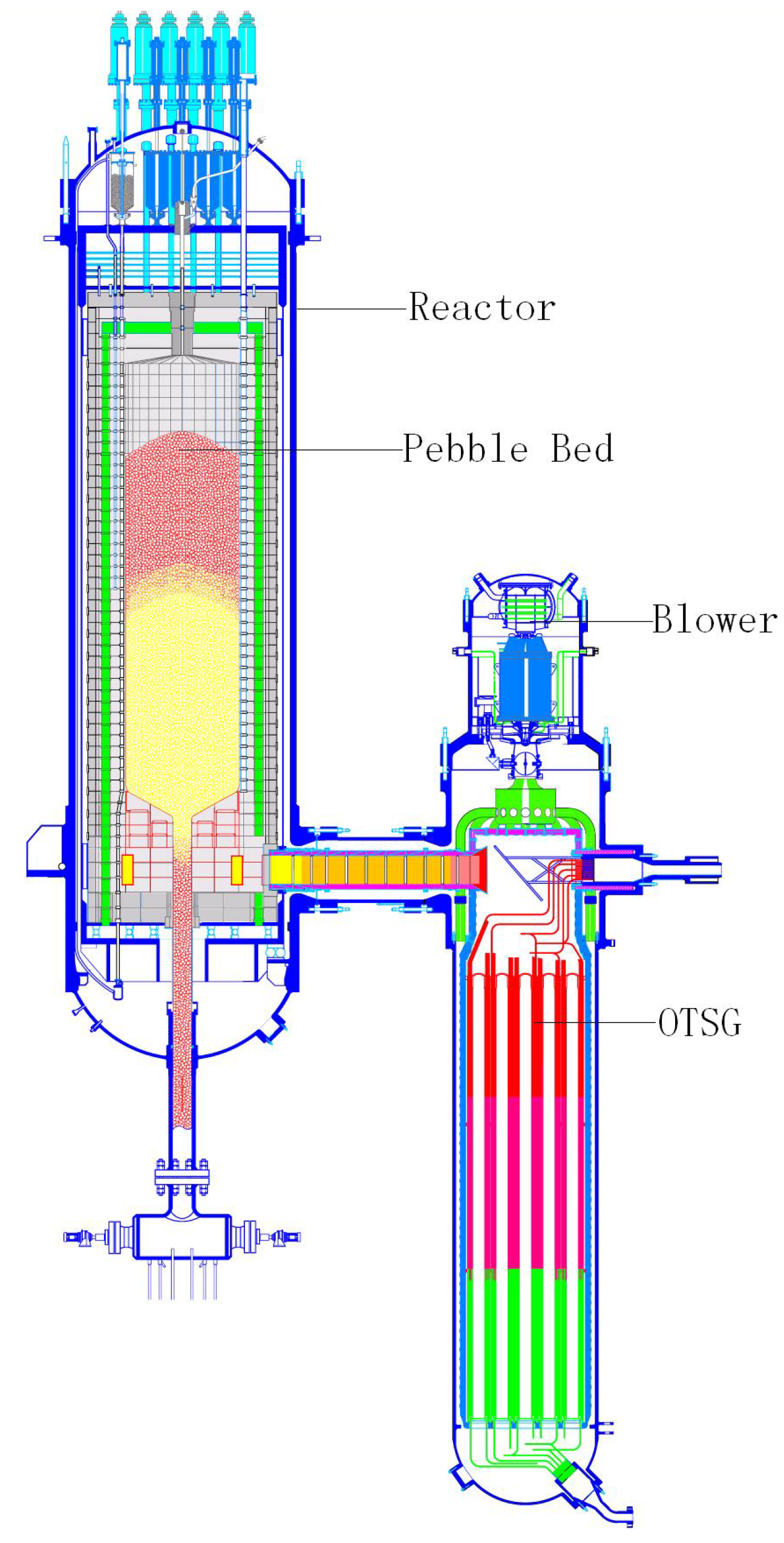This configuration not only guarantees the vital inherent safety properties but also provides the competitive economic characteristics [8]. The reactor core and the OTSG are arranged side by side, as illustrated in Figure 1, and are housed in a steel pressure vessel, respectively. The two vessels are connected to each other by means of a hot gas duct. The cold helium (about 250 °C) enters the main blower located on the top of the OTSG vessel, and is pressurized before flowing into the coaxial pipe of the hot gas duct. It enters the channels in the reflector of the core from bottom to top, and then passes through the pebble-bed core from top to bottom where it is heated to a temperature of about 750 °C. The hot helium leaves the hot gas chamber in the bottom reflector and flows into the OTSG through the hot gas duct. Both of the NSSSs are connected to a steam header that delivers steam to a 200 MW_e turbo-generator. Safe, stable and efficient operation is a key requirement for any nuclear reactors and also certainly for the MHTGRs, and power-level regulation is one of the key techniques that guarantee economic performance.

Figure 1. Schematic diagram of the HTR-PM’s NSSS.

Figure 1. Schematic diagram of the HTR-PM’s NSSS.

The basic principle of the power-level control is the modulation of the rate of insertion and withdrawal of the control rods to regulate power output at a demand value using core power and average coolant temperature error signals computed from measurements. Moreover, power-distribution control is another aspect of power regulation as power-level control is, and the goal of the power-distribution control is to guarantee that the neutron concentration at each position cannot surpass its upper bounds. The main task of power-distribution control is to suppress the xenon oscillation. However, with proper design of the reactor core and fuel cycle, the xenon oscillation cannot result in a power-distribution swing inside the MHTGR core. The main design data of the HTR-PM reactor core, which is a typical MHTGR core, is given in Table 1 [7]. As we can see from Table 1, the active area of the HTR-PM reactor core has a small diameter of 3 m and a large height of 11 m. The small diameter of the reactor guarantees that there is no severe xenon oscillation along the radial direction. Moreover, to obtain the most uniform power density distribution possible along the axial direction, the spherical fuel elements pass through the core approximately 15 times before reaching their final burn-up [4]. Because of the slim core shape and multi-passing-through fuel cycle type of the pebble-bed high temperature gas-cooled reactor, xenon oscillation cannot induce an axial power density swing [9]. Since there is no severe power-density oscillation inside the MHTGRs such as the HTR-PM reactor, power-level control is the most crucial for the regulation of MHTGR.

At present, classical output feedback power-level control still dominates commercial nuclear power plant operation. With the development of current high speed microprocessors in the past decades, however, it is now possible to apply more modern control strategies for improving control performance. Many promising power-level controllers have been developed during the past two decades.

Table 1. Main design data of the HTR-PM reactor core.

Parameters	HTR-PM
Number of NSSS modules	2
Thermal power (MW)	2 × 250
Primary helium pressure (MPa)	7
Core outlet temperature (°C)	250
Core inlet temperature (°C)	750
Primary helium flow-rate (kg/s)	96
Active core diameter (cm)	300
Equivalent active core height (cm)	1100
Fuel enrichment (%)	8.9
Number of fuel elements in one reactor core	420,000

Table 1. Main design data of the HTR-PM reactor core.

Parameters	HTR-PM
Number of NSSS modules	2
Thermal power (MW)	2 × 250
Primary helium pressure (MPa)	7
Core outlet temperature (°C)	250
Core inlet temperature (°C)	750
Primary helium flow-rate (kg/s)	96
Active core diameter (cm)	300
Equivalent active core height (cm)	1100
Fuel enrichment (%)	8.9
Number of fuel elements in one reactor core	420,000

Combining the characteristics of the static output and state feedback control, Edwards et al. established a novel control configuration called the state feedback assisted classical control (SFAC) [10]. The SFAC is an approach which uses the concept of state feedback to modify the load signal for an embedded classical output feedback controller, and is also useful in existing plant implementation because it leaves in place current classical feedback loops. To improve the robustness of the closed-loop system, the linear quadratic Gaussian regulator with loop transfer recovery (LQG/LTR) was applied to the power-level stabilization under the SFAC configuration [11,12]. Since the SFACs are essentially linear control strategies guaranteeing closed-loop stability near the operating point, it is very necessary to develop nonlinear power-level controllers. Shtessel gave a nonlinear power-level regulator composed of a static state feedback sliding mode controller and a sliding mode state observer for space nuclear power system TOPAZ II [13]. As an alternative to the model-based controller design, many soft-computing approaches, such as artificial neural networks, fuzzy sets and genetic algorithms (GA), have been applied to power-level or control. A power-level controller for nuclear reactors using two diagonal recurrent neural networks (DRNN) was presented, and robustness and adaptive capability of the DRNN was also demonstrated [14]. Na et al. presented a fuzzy model predictive controller (MPC) optimized by GA for the power-level control of pressurized water reactors (PWRs) [15]. Huang et al. proposed a robust multi-input multi-output (MIMO) power-level control based on fuzzy-adapted recursive sliding mode control technique for an advanced boiling water reactor (ABWR) for regulating the nuclear power, the water-level and the turbine throttle pressure simultaneously [16]. From the foregoing introduction, the SFAC is designed based on the linearized reactor dynamic model, and it only guarantees both closed-loop stability and control performance near the operation point. Since the HTR-PM is often operated in the large power maneuver mode, the SFAC-like linear controllers are not optimal for this power plant. The nonlinear power-level regulation strategy based on the sliding mode controller and observer is very complex and is also not easy for the engineering implementation. The performance of those intelligent power controllers is determined by the training samples to a great extent. Since the HTR-PM is still under design and construction, there were no training samples obtained from the running data, and it is not feasible to design an intelligent power-level controller for the HTR-PM.

Recently, control theory of generalized Hamiltonian systems has been investigated extensively [17]. The basic idea of this theory involves adding a dissipative part through feedback so that the closed-loop system is globally asymptotic stable. The approach is implemented in two steps: realization and feedback dissipation. In realization, the dynamics of a given nonlinear system is decomposed into conservative, dissipative and emanative parts [18,19]. In the second step, the emanative part of the dynamics is restrained by feedback for asymptotic closed-loop stability [20,21,22]. This control theory has been successfully applied to power system regulation [23], nuclear reactor state-observation [24], water-level control of U-tube steam generators (UTSGs) [25], etc. Since the dynamics of the HTR-PM are highly nonlinear, and the system parameters also vary with the power-level extensively, it is quite necessary to design a simple power-level regulator which guarantees globally asymptotic closed-loop stability. Stimulated by this, an output feedback dissipation power-level controller is given in this paper. This newly built power-level regulator not only has the virtues of globally asymptotically stabilizing capability and easy implementation, but also needs only the measurements of the nuclear power, average temperature of the helium inside reactor core and control rod positions as inputs. Moreover, this controller is simplified to the classical proportional output feedback control if the control rod dynamic model can be well approximated by an integrator. Numerical simulation results show the performance of this new controller and its simplified version.

The rest part of this paper is organized as follows. The nonlinear state-space model for power-level controller design is given in Section 2. The theoretical control problem is formed in the beginning of Section 3, and then through solving this problem in Subsections 3.2 and 3.3, the design approach of the power-level controller is then established. In Subsection 3.4, this approach is applied to design the power-level regulator for the MHTGR. Numerical simulation results with some discussion are given in Section 4, and the corresponding concluding remarks are given in Section 5.

2. Nonlinear State-Space Model

For designing the power-level control of the MHTGR, the dynamic model of the reactor core is adopted from the point kinetics with one equivalent delayed neutron group with reactivity induced by the variation of the average fuel and reflector temperatures, which can be written as [26,27]:

(1)

where the meaning of the variables in Equation (1) is given in Table 2.

To design the power-level control law, the deviations of the actual values of n_r, c_r, T_c, T_d, T_din, T_r and ρ_r from equilibrium values n_r0, c_r0, T_c0, T_d0, T_din0, T_r0 and ρ_r0 are concerned, which are defined as:

(2)

Table 2. Meaning of the variables in Equation (1).

Variable	Meaning
nr	neutron concentration relative to the concentration at rated condition
cr	relative concentration of the delayed neutron precursor
β	fraction of delayed fission neutrons
Λ	effective prompt neutron lifetime
λ	effective radioactive decay constant of the delayed neutron precursor
αc	reactivity coefficients of the fuel temperature
αr	reactivity coefficients of the reflector temperature
Tc	average temperature of the fuel elements
Td	average temperature of the helium inside the core
Tdin	inlet helium temperature of the core
Tr	average temperature of the reflector
Tc,m	initial equilibrium value of Tc
Tr,m	initial equilibrium value of Tr
Ωcd	heat transfer coefficient between fuel and coolant
Ωcr	heat transfer coefficient between the fuel elements and the reflector
M	mass flow-rate times heat capacity of the coolant
P0	rated power level
ρr	reactivity due to the control rods
μd	total heat capacity of the fuel elements
μc	total heat capacity of the reactor coolant
Gr	total differential worth of control rods
zr	speed signal of the control rods

Table 2. Meaning of the variables in Equation (1).

Variable	Meaning
nr	neutron concentration relative to the concentration at rated condition
cr	relative concentration of the delayed neutron precursor
β	fraction of delayed fission neutrons
Λ	effective prompt neutron lifetime
λ	effective radioactive decay constant of the delayed neutron precursor
αc	reactivity coefficients of the fuel temperature
αr	reactivity coefficients of the reflector temperature
Tc	average temperature of the fuel elements
Td	average temperature of the helium inside the core
Tdin	inlet helium temperature of the core
Tr	average temperature of the reflector
Tc,m	initial equilibrium value of Tc
Tr,m	initial equilibrium value of Tr
Ωcd	heat transfer coefficient between fuel and coolant
Ωcr	heat transfer coefficient between the fuel elements and the reflector
M	mass flow-rate times heat capacity of the coolant
P0	rated power level
ρr	reactivity due to the control rods
μd	total heat capacity of the fuel elements
μc	total heat capacity of the reactor coolant
Gr	total differential worth of control rods
zr	speed signal of the control rods

Moreover, we define:

(3)

(4)

and:

(5)

Then dynamic model (1) can be rewritten as:

(6)

and Equation (6) can also be written as the following vector form:

(7)

where:

(8)

and:

(9)

Here the output function of (7) is chosen as:

(10)

where output y can be calculated from the measurements of n_r and T_d. In the following parts of this paper, the power-level control is designed based on the nonlinear state-space model composed of (7) and (10).

3. Design of the Power-Level Controller

In this section, a control problem is formulated from the requirement of the power-level controller design for MHGTRs, and then this problem is solved theoretically in two steps. Finally, the results are applied to design the power-level regulator.

3.1. Control Problem Formulation

From the nonlinear state-space model given in the above section, in order to design the power-level regulator for MHTGRs, we should first solve the following control problem:

Problem. How to design a controller which guarantees the globally asymptotic closed-loop stability for the single-input-single-output (SISO) nonlinear systems taking the form as:

(11)

where x ∈ Rⁿ and ξ ∈ R constitutes the state space, u ∈ R is the control input, y ∈ R is the system output.

3.2. Introduction to the Concepts of Feedback Dissipation Control and Zero-State Detectability

Before giving the design approach of the output feedback stabilizer for system (11), some useful concepts are firstly introduced as follows.

Consider a nonlinear system taking the form as:

(12)

where x ∈ Rⁿ is the system state vector, u ∈ R^p is the control input, y ∈ R^q is the system output, and f(O) = O. Here, system (12) denotes an actual engineering system such as a mechanical system, an electrical system, a thermodynamic system or a nuclear power plant. Usually, the energy of a given engineering system can be represented by a semi-positive function H(x,t), which is called the Hamiltonian function. Apparently, means that the energy of this system becomes smaller and smaller, and then the system is called to be dissipative. Moreover, the system is emanative if , and the system is conservative if .

From the viewpoint of system control, the Hamiltonian function is quite similar to a Lyapunov function, and if the system is dissipative, then the system state converges to . For a given Hamiltonian function H(x,t), the dissipation of system (12) can be guaranteed by control input u. Here, u is said to be a feedback dissipation control if:

(13)

is satisfied for H(x,t) ≠ 0, i.e., the closed-loop system is dissipative. If u = u(x), then it is said to be a state-feedback dissipation control. If u = u(y), then it is called an output-feedback dissipation control.

Though a Hamiltonian function looks like a Lyapunov function, it is really not a Lyapunov function because it is not strictly positive-definite. Thus, the concept of zero-state dectectability is introduced here for stability analysis based upon the Hamiltonian function. System (12) is said to be zero-state detectable if and ( ) implies:

(14)

3.3. Design Approach of Feedback Dissipation Control

In order to solve the problem raised in Subsection 3.1, the design process of the asymptotical control for system (11) is partitioned in the following two steps:

Step 1:

The first step is to design a feedback dissipation control law for SISO subsystem:

(15)

based on regarding state-variable ξ as a virtual control input.

As discussed in Subsection 3.2, for a given Hamiltonian function, ξ is a feedback dissipation control of system (15) if inequality (13) is satisfied. Here, if the corresponding Hamiltonian function satisfies:

(16)

where:

(17)

then inequality (13) can be rewritten as:

(18)

Moreover, in order to guarantee , we can choose ξ as:

(19)

where K(x) is positive. Substitute Equations (19) to (18):

(20)

From Equation (20), when H(x,t) ≠ 0, i.e., y ≠ 0, we can choose a large enough K(x) so that , which means that (19) is an output feedback dissipation controller for system (15). Furthermore, state-vector x will finally converge to:

(21)

When H(x, t) ≡ 0, i.e., ξ ≡ y ≡ 0, state-vector x ∈ Γ. As we have discussed in Subsection 3.2, if system (15) is zero-state detectable, then from Equation (14), state-vector x converges to the origin asymptotically. Thus, feedback dissipation control (19) can also guarantee globally asymptotic stability if system (15) is zero-state detectable.

Step 2:

The second step is to develop a feedback controller which guarantees globally asymptotical closed-loop stability for entire system (11) based on the above discussion and the well-known backstepping approach [28,29]. Here, the backstepping is a strong nonlinear controller design method, whose the key idea is to start with a system that is stabilizable with a known feedback law, and then add this control input to an integrator. For the augmented system, a new stabilizing feedback law is explicitly designed, and so on [28].

From the discussion in the first step, the most important thing of designing a feedback dissipation controller is choosing a proper Hamiltonian function and guaranteeing its asymptotical convergence to the origin through feedback.

Here, we want to give a Hamiltonian function for entire system (11) based on Hamiltonian function (16) for subsystem (15). In order for this, define ξ_des as the reference control input for (15) that determined by (19), and define e_ξ as the error between the actual and referenced value of ξ, i.e.,:

(22)

Then, based on the key idea of the backstepping approach, the Hamiltonian function for entire system (11) can be chosen as:

(23)

Similar to the method in step one, differentiate entire Hamiltonian function (23) along the trajectory given by (11) and (19), and we have:

(24)

From Equation (24), if we choose the feedback controller as:

(25)

where F is a positive scalar, then:

(26)

In case of y ≠ 0, from the discussion in the first step and Equation (24), we have:

(27)

If e_ξ = 0, then we have:

(28)

If e_ξ ≠ 0, inequality (28) can be also satisfied if we choose a large enough F.

In case of y = 0, from Equation (16) and the zero-state detectability of subsystem (15), we have:

(29)

and:

(30)

From Equations (29) and (30):

(31)

If e_ξ = 0, then the state vector is just at the origin. If e_ξ ≠ 0, inequality (28) can be guaranteed by choosing a positive F. Therefore, if subsystem (15) is zero-state detectable and equation (16) is satisfied, then control law (25) guarantees the globally asymptotic closed-loop stability if ξ_des satisfies (19) and positive scalar F is large enough.

3.4. Design of Power-Level Regulator Based on Feedback Dissipation Approach

In this subsection, we shall design the power-level control for high temperature gas-cooled reactors such as the HTR-PM, and the idea is using the method given in Subsection 3.3 iteratively for two times. From the results given in Subsection 3.3, if the Hamiltonian function has been chosen, then the system output and the feedback dissipation control are both determined. It is noteworthy that different Hamiltonian functions usually result in different system output and feedback dissipation controllers. The design process of the power-level control is split into the following three steps.

Step 1:

For the high temperature gas-cooled reactors whose dynamics is described by Equations (7)–(9), we firstly consider the following subsystem:

(32)

where variables x, ξ are given by Equations (3) and (4) respectively, and vector-valued functions f(x) and g(x) are determined by (8) and (9) respectively.

If the Hamiltonian function of subsystem (32) is chosen as:

(33)

then the corresponding system output is:

(34)

Substitute Equations (34) to (19), the feedback dissipation controller corresponding to Hamiltonian function (33) can be written as:

(35)

where K₁(x) is a positive-definite function. Moreover, if we choose K₁(x) as:

(36)

where K₁ is a large enough positive scalar, then (35) can be rewritten as:

(37)

If we choose virtual control ξ as:

(38)

then closed-loop system formed by (32) and (38) can represented as:

(39)

where:

(40)

Based on the discussion in Subsection 3.3, subsystem (39) has the property:

i.e.,

(41)

when ξ₂ ≡ 0.

Step 2:

In the following, we shall design ξ₂ so that globally asymptotic closed-loop stability is guaranteed. Similar to the design of ξ₁, we firstly choose the Hamiltonian function of subsystem (39) as:

(42)

Then the corresponding system output and feedback dissipation controller are respectively given by:

(43)

and:

(44)

where:

(45)

and K₂ is a large enough positive scalar.

From Equations (37) and (44), total virtual control (38) satisfies:

(46)

where:

(47)

and H₁(x,t) and H₂(x,t) satisfy Equations (33) and (42) respectively. From the design approach given in Subsection 3.3, it is clear that ξ is the feedback dissipation controller corresponding to Hamiltonian function H(x,t). Thus, the closed-loop system determined by (32) and (46) has the property:

(48)

which is equivalent to:

(49)

Based on the approach given in Subsection 3.3, we have designed feedback dissipation control (46) so that the closed-loop system has the property. Moreover, regulator (46) guarantees the globally asymptotic closed-loop stability if closed-loop system formed by (39), (44) and (43), i.e.,

(50)

is zero-state detectable.

Actually:

(51)

means:

(52)

and from (41), we can see that:

(53)

Substituting (41) into (6.2), we have:

(54)

Moreover, from equations (6.3), (6.4) and (52), we can also calculate that:

(55)

Based on (55) and (6.3):

(56)

if:

(57)

Since α_c < 0, α_r > 0 and the left side of (57) is positive, inequality (57) is easily satisfied. Then from (55) and (56), it is clear that:

(58)

From (58), it is clear that system (50) is zero-state detectable. Thus, control (46) makes the closed-loop system globally asymptotically stable.

Furthermore, if the entire system output is chosen as:

(59)

where y₁ and y₂ are respective determined by Equations (34) and (43), then y ≡ O results in:

(60)

Equation (60) certainly leads to (54), (56) and (58), which means that zero-state detectability is an inherent property for this system.

Step 3:

Based on the approach given in Subsection 3.3, the control rod speed signal is:

(61)

where:

(62)

and:

(63)

If the rod dynamics can be well described by an integrator, then controller (61) can be simplified to:

(64)

which is just the proportional feedback controller. In the next section, the performance of controllers (61) and (64) will be studied through numerical simulation.

4. Numerical Simulation with Discussion

To show the feasibility and performance of controllers (61) and (64), these two controllers are both applied to the power-level of a NSSS of the HTR-PM power plant in this section. The influence of the dead-zone of the rod speed to the control performance is illustrated and analyzed. The condition that simplified controller (64) can well approximate feedback dissipation regulator (61) is also given.

4.1. Description of the Numerical Simulation

The numerical simulation model, whose schematic view is given in Figure 2, is developed based on Visual C++. Since the height-to-diameter ratio of the HTR-PM is nearly 4, the classical point kinetics model is not suitable for use to build the simulation code of HTR-PM. By dividing the active core region vertically into 10 parts, a nodal neutron kinetics model and its corresponding thermal-hydraulic model are used to establish the simulation model of the reactor core [26]. Here, the OTSG is adopted the moving boundary model [30].

Figure 2. Nodalization for the NSSS of the HTR-PM.

Figure 2. Nodalization for the NSSS of the HTR-PM.

4.2. Simulation Results

In the simulation, the following two case studies are done to show the control performance of feedback dissipation power-level controller (61) and simplified proportional feedback controller (64).

Case A (large power drop): power-level changes linearly from 100% to 50% in 5 min.

• Use feedback dissipation power-level controller (PLC) (61).
• Use simplified proportional feedback power-level controller (64).

Case B (large power lift): power-level changes linearly from 50% to 100% in 5 min.

• Use feedback dissipation power-level controller (61).
• Use simplified proportional feedback power-level controller (64).

The feedback gains are chosen to be k_n = 0.1, k_T = 0.0002 and k_ρ = 1. Moreover, the dynamic model of the control rods utilized in the simulation is different with that for controller design. The rod dynamics model for simulation has a rod speed dead zone, while that for controller design has no dead zone of rod speed. The control rod dynamics with rod speed dead-zone can be written as:

(65)

where z_r,d is just the output of the rod speed dead-zone:

(66)

and positive scalar v_d denotes the size of the dead-zone. Numerical simulation results using (61) and (64) with different values of v_d are given as follows:

(1)

Power-level drop

In this test, the power demand decreases down from 100% to 50% linearly with a speed of 10%/min. Corresponding to the power demand drop, both the error between the actual and the demanded power-levels and that between the actual and the referenced values of average coolant temperature become larger than before. These error signals stimulate the power-level controller to insert the control rod in order to weaken these two error signals. If (61) is adopted in the simulation, then the responses of the nuclear power, the average temperature of the fuel elements, the average helium temperature and the control rod speed generated by the power-level controller are all illustrated in Figure 3. If simplified proportional control (64) is utilized, then the corresponding responses of the process variables are given in Figure 4.

Figure 3. Power drop controlled by feedback dissipation PLC. (a) Relative nuclear power-level; (b) Average temperature of fuel elements; (c) Outlet helium temperature of the reactor; (d) Control rod speed signal.

Figure 3. Power drop controlled by feedback dissipation PLC. (a) Relative nuclear power-level; (b) Average temperature of fuel elements; (c) Outlet helium temperature of the reactor; (d) Control rod speed signal.

Figure 4. Power drop controlled by proportional PLC. (a) Relative nuclear power-level; (b) Average temperature of fuel elements; (c) Outlet helium temperature of the reactor; (d) Control rod speed signal.

Figure 4. Power drop controlled by proportional PLC. (a) Relative nuclear power-level; (b) Average temperature of fuel elements; (c) Outlet helium temperature of the reactor; (d) Control rod speed signal.

(2)

Power lift

As the power demand signal rises linearly from 50% to 100% in 5 min, the error signals in both the nuclear power and the average helium temperature cause the power regulator to generate positive speed control action and lift the control rod to reduce this error. The computed responses of reactor process variables to the control action (61) and (64) are illustrated in Figure 5 and Figure 6, respectively.

Figure 5. Power lift controlled by feedback dissipation PLC. (a) Relative nuclear power-level; (b) Average temperature of fuel elements; (c) Outlet helium temperature of the reactor; (d) Control rod speed signal.

Figure 5. Power lift controlled by feedback dissipation PLC. (a) Relative nuclear power-level; (b) Average temperature of fuel elements; (c) Outlet helium temperature of the reactor; (d) Control rod speed signal.

Figure 6. Power lift controlled by proportional PLC. (a) Relative nuclear power-level; (b) Average temperature of fuel elements; (c) Outlet helium temperature of the reactor; (d) Control rod speed signal.

Figure 6. Power lift controlled by proportional PLC. (a) Relative nuclear power-level; (b) Average temperature of fuel elements; (c) Outlet helium temperature of the reactor; (d) Control rod speed signal.

4.3. Discussion

From Figure 3 and Figure 4, if there is no dead-zone of the controd rod speed, then both feedback dissipation power-level controller (61) and simplified proportional controller (64) can guarantee globally closed-loop asymptotic stability. However, if there exists a nonzero dead-zone, then there is a very evident difference between the performance of (61) and that of (64). As shown in Figure 3 and Figure 4, even when the rod speed dead-zone is a bit large, the power regulator (61) can still provide globally asymptotic closed-loop stability. The simplified controller (64) cannot guarantee asymptotic closed-loop stability even when the dead-zone is quite small. The reason is given as follows: the simplified control policy (64) assumes that the modeling error of control rod dynamics is small enough to be neglected. The nonzero deadzone violates this assumption and results in the unsatisfactory performance of the controller (64). Based on Figure 3d and Figure 4d, if the modeling error is large and the simplified control law is utilized, then the corresponding rod speed signal enters the deadzone earlier than that generated by feedback dissipation controller (61). Because the speed signal determined by the second term in the right side of Equation (64) is too small to make the total speed signal escape from the dead-zone, the error of the average helium temperature of reactor core cannot ever be zero. However, due to the existence of the compensating term [i.e., the 3rd term in the right side of Equation (61)], the rod speed signal given by (61) remains outside the deadzone much longer than that given by (64), and the errors between the actual and referenced values of the process variables go to zero asymptotically. Though feedback dissipation power-level regulator (61) can still guarantee globally asymptotic closed-loop stability, the control performance is deteriorated if the speed dead-zone is enlarged. From Figure 3, the overshoots of the process variables are larger if the dead-zone is enlarged, i.e., there is a trade-off between the robust globally asymptotical stability and control performance.

From Figure 5 and Figure 6, the simplified proportional power-level controller (64) can only guarantee the asymptotic closed-loop stability if there is no dead-zone, while the feedback dissipation regulator (61) can drive the process variables asymptotically to their reference values even when the dead-zone is a bit large. Similar to the case of power drop, this can also be explained through exploring the function of the compensating term. It is clear that the compensating term can enlarge the period during which the rod speed signal stays outside the dead-zone. Moreover, if regulator (61) is adopted, then it is can be seen that the dead-zone is larger, the overshoots of the process variables become larger.

Based on these simulation results, it is clear that modeling uncertainty of the control rod dynamics has a strong influence to both control performance and closed-loop stability. The main merit of regulator (61) is the capability of guaranteeing the globally asymptotic closed-loop stability with the existence of modeling error in the control rod dynamics. However, the main shortcoming of (61) is just induced by its merit.

From the above discussion, δρ_r is computed based upon the measurements of the control rod positions, and applying controller (61) in practical engineering can complicate the reactor power control system. However, simplified controller (64) only needs the measurements of the nuclear power and the outlet and inlet helium temperatures, which means that the merit of controller (64) is its simplicity. In summary, if the modeling error in the control rod dynamics is small enough to be omitted, then using simplified proportional power-level controller (64) is enough. Otherwise, feedback dissipation power-level controller (61) must be adopted to make the closed-loop system globally asymptotically stable.

5. Conclusions

Because of its inherent stability and safety, the modular high temperature gas-cooled reactor is a strong candidate for the next generation of nuclear energy systems. The large variability in power level anticipated for this type of plant can result in diminished performance if classical feedback control theory is applied. Large-scale asymptotic closed-loop stability can be provided by nonlinear controllers. Effective wide-range power-level regulation based on feedback dissipation and backstepping is demonstrated in this paper. Implementing this regulator needs the measurements of the nuclear power, the average helium temperature of the reactor core and the rod positions. The most advanced feature of this newly-built power-level regulator is the ability to guarantee the globally asymptotic close-loop stability by the use of the intrinsic property of the MHTGR dynamics, i.e., the zero-state detectability. This causes the new regulator to display both the characteristics of simple expression and satisfactory performance. Both theoretical analysis and numerical study show that this controller can not only guarantee globally asymptotic stability, but also be quite robust to the modeling uncertainty of the rod dynamics. Moreover, if the modeling uncertainty of the rod dynamics is small enough to be neglected, then this newly built power-level control is simplified to the classical proportional feedback regulator that only needs to measure the nuclear power and helium temperature.