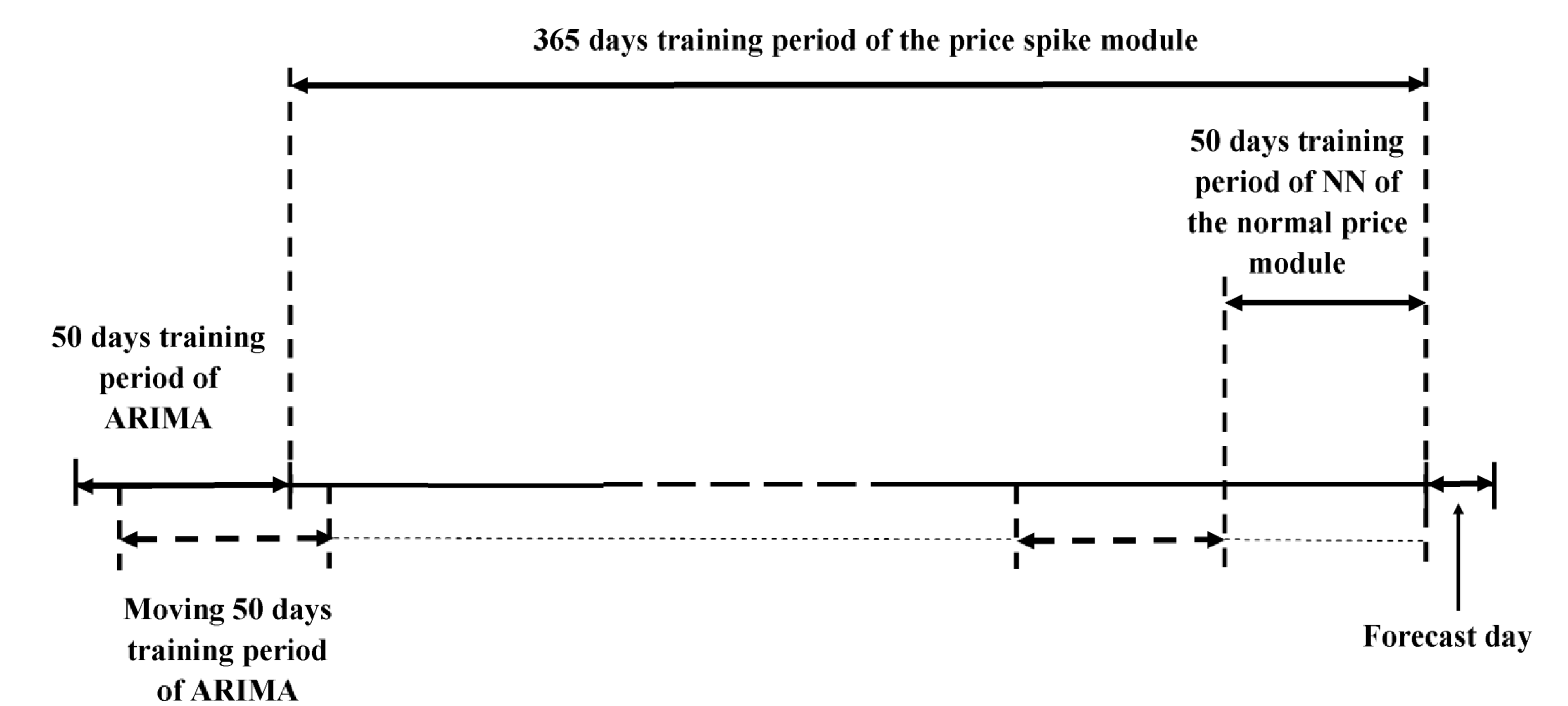
For examination of the proposed method, the real hourly data of the Finnish day-ahead energy market are considered. The electricity price, demand and supply historical data over the period from November 2008 to December 2009 are used to establish the initial training data sample set. The data over the period from January 2010 to December 2010 are used as the test set.
6.3. Numerical Results
The obtained results of the two-step feature selection algorithm implemented for the compound classifier, the k-NN and the NN to predict prices in the Finnish day-ahead energy market for a single forecast day, 5 January 2010, are presented in
Table 2 and
Table 3. Since electricity price spikes have a very volatile stochastic nature with respect to the normal price time series, regular and periodic behaviour of price spikes are not so obvious (see
Table 2). Otherwise, variables of the short-run trend (e.g., A3
p,h−1, D3
p,h−2), daily periodicity (e.g., A3
p,h−25, D3
p,h−24) and weekly periodicity (e.g., A3
p,h−169, A3
d,h−169) are among the selected input features to forecast normal price wavelet components (see
Table 3).
Table 2.
Selected inputs for the three classification approaches of the compound classifier and the k-NN for a single forecast day, 5 January 2010.
Table 2.
Selected inputs for the three classification approaches of the compound classifier and the k-NN for a single forecast day, 5 January 2010.
| Engine | V0/V1/V2 | Parameter | Selected candidates |
|---|
| RVM | 0.43/0.46/0.64 | σRVM = 0.13 | A3p_arima,h, A3p,h−1, A3p,h−2, A3p,h−4, A3p,h−5, A3p,h−6, A3p,h−7, D1p_arima,h, D1p,h−1, D1p,h−2, D1p,h−3, ph−1, ph−2, ph−3, ph−4,dh, dh−2, dh−46, dh−72, suph, indh, indd |
| PNN | 0.47/0.50/0.78 | σPNN = 0.03 | A3p_arima,h, A3p,h−1, A3p,h−2, A3p,h−3, A3p,h−4, A3p,h−5, A3p,h−6, A3p,h−22, D1p_arima,h, D1p,h−1, D1p,h−2, D1p,h−3, D1p,h−4, D1p,h−5, ph−2, ph−3, ph−4, dh−2, dh−21, dh−22, suph−2, indh, indd, inds |
| DT | 0.42/0.48/0.61 | Ntree = 100 | A3p_arima,h, A3p,h−1, A3p,h−2, A3p,h−4, A3p,h−5, A3p,h−6, A3p,h−7, D1p,h−1, D1p,h−2, D1p,h−3, ph−1, ph−2, ph−3, ph−4, ph−5, dh, dh−4, dh−19, dh−69, dh−73, indh, indd |
| k-NN | -/0.45/0.56 | k = 3 | A3p_arima,h, A3p,h−2, A3p,h−9, A3p,h−15, A3p,h−21, D1p,h−2, D1p,h−5, D1p,h−7, D1p,h−8, D1p,h−16, ph−1, ph−3, ph−7, ph−52, dh−190, indh, indd, inds |
Table 3.
Inputs selected by the two-step feature selection to predict the normal price wavelet components for the NN for a single forecast day, 5 January 2010.
Table 3.
Inputs selected by the two-step feature selection to predict the normal price wavelet components for the NN for a single forecast day, 5 January 2010.
| Subseries | Nh/V1/V2 | Selected candidates |
|---|
| A3 p | 4/0.52/0.71 | A3p_arima,h, A3p,h−1, A3p,h−3, A3p,h−4, A3p,h−16, A3p,h−21, A3p,h−25, A3p,h−72, A3p,h−97, A3p,h−121, A3p,h−144, A3p,h−169, A3d,h−8, A3d,h−10, A3d,h−11, A3d,h−42, A3d,h−91, A3d,h−98, A3d,h−141, A3d,h−169, ph−72, ph−95, ph−97,ph−120 |
| D3 p | 7/0.47/0.81 | D3p_arima,h, D3p,h−1, D3p,h−2, D3p,h−11, D3p,h−24, D3p,h−48, D3p,h−60, D3p,h−96, D3d,h−12, D3d,h−47, D3d,h−71, D3d,h−143 |
| D2 p | 4/0.41/0.74 | D2p_arima,h, D2p,h−1, D2p,h−7, D2p,h−8, D2p,h−24 |
| D1 p | 6/0.15/0.85 | D1p_arima,h, D1p,h−6, D1p,h−24, D1p,h−30, D1p,h−48, D1p,h−72, D1p,h−94, D1p,h−120, D1p,h−157 |
In this paper, Adapted Mean Average Percentage Error (AMAPE) proposed in [
10] was considered to evaluate the forecast results:
where
PiACTUAL and
PiFOREC are actual and forecast values of hour
i, respectively; and
T is the number of predictions.
In addition, two performance measures that are spike prediction accuracy and spike prediction confidence proposed in [
17] are used to reliably assess the performance of the compound classifier.
Spike prediction accuracy is a ratio of the number of correctly classified spikes (
Ncorr) to the number of actual spikes (
Nsp):
This measure was introduced because the ability to correctly predict spike occurrence is the subject of greatest concern.
Spike prediction confidence aims to account for the uncertainties and risks carried within the forecast. Spike prediction confidence is described as:
where
Ncorr is the number of correctly classified spikes and
Nas_sp is the number of observations classified as spikes. As the classifier may misclassify some nonspikes as spikes, this definition is used to assess the percentile in which the classifier makes this kind of a mistake.
Only few research works have considered price forecasting in the Finnish day-ahead energy market and it was not possible to find price forecast methods considering the above-mentioned test period for price forecast. Therefore, the overall accuracy of the proposed method is compared with some of the most popular price forecast techniques applied for case studies of energy markets of other countries: seasonal ARIMA [
5,
44,
50]; WT+ARIMA [
26,
28]; NN [
6,
50]; WT + NN [
11]. Additionally, WT + ARIMA + NN, which has not been found in the literature is among competitive techniques. To demonstrate the efficiency of the proposed methodology, its obtained results for the Finnish day-ahead energy market in year 2010 are shown in
Table 4 with corresponding results obtained from five other prediction techniques.
In the WT + NN and WT + ARIMA + NN models separate NNs with the LM algorithm are applied for each price wavelet component. For a fair comparison, NN, WT + NN and WT + ARIMA + NN have historical and forecasted demand data among the candidate inputs. Feature selection analysis based on the proposed two-step feature selection is utilized for all examined models. The adjustable parameters of the competing models are fine-tuned by the proposed search procedure. It should be noted that among the competing examined models, only the WT + ARIMA + NN has preliminarily predicted price values in its set of candidate inputs i.e., the NN uses predictions from ARIMA as the candidate input.
As seen from
Table 4, the AMAPE values corresponding to the proposed strategy are lower than the values obtained from other examined methods. The accuracy improvement of the proposed method with respect to seasonal ARIMA, WT + ARIMA, NN, WT + NN, and WT + ARIMA + NN in terms of AMAPE is 45.88% [(1 − 8.08/14.93) × 100%], 19.44% [(1 − 8.08/10.03) × 100%], 35.46% [(1 − 8.08/12.52) × 100%], 32.55% [(1 − 8.08/11.98) × 100%], and 16.36% [(1 − 8.08/9.66) × 100%], respectively. It can also be seen that the use of WT results in an improvement in the model accuracy. This improvement in ARIMA in comparison with WT+ARIMA in terms of AMAPE is 32.82% [(1 − 10.03/14.93) × 100%]. For the NN in comparison with WT+NN, this value is 4.31% [(1 − 11.98/12.52) × 100%]. The results also confirm the efficiency of the hybrid methodology with linear and nonlinear modeling capabilities (WT + NN
versus WT + ARIMA + NN) where the improvement is 19.37% [(1 − 9.66/11.98) × 100%].
Table 4.
AMAPE (%) obtained from different techniques for price forecasts in the Finnish day-ahead energy market of year 2010.
Table 4.
AMAPE (%) obtained from different techniques for price forecasts in the Finnish day-ahead energy market of year 2010.
| Type | Seasonal ARIMA | WT + ARIMA | NN | WT + NN | WT + ARIMA + NN | Proposed method |
|---|
| Normal | 10.53 | 7.53 | 8.17 | 8.01 | 7.18 | 5.89 |
| Spikes | 55.76 | 40.51 | 46.33 | 44.22 | 37.72 | 32.91 |
| Overall | 14.93 | 10.03 | 12.52 | 11.98 | 9.66 | 8.08 |
It is expected that implementation of the proposed iteration strategy increases the accuracy of the overall price prediction. Detailed results of the proposed iteration strategy for the four test weeks of the Finnish day-ahead energy market of year 2010 are shown in
Table 5. These test weeks are related to dates 1−7 January 2010, 8−14 January 2010, 29 January−4 February 2010, 5−11 February 2010, respectively, and indicate periods of high volatility in energy price series. Iteration 0 in
Table 5 represents the obtained results from the initial forecasting model.
Table 5.
Accuracy of the proposed iteration procedure in terms of AMAPE (%) for the four test weeks of year 2010.
Table 5.
Accuracy of the proposed iteration procedure in terms of AMAPE (%) for the four test weeks of year 2010.
| Iteration | Week1 | Week2 | Week5 | Week7 |
|---|
| 0 | 17.46 | 37.27 | 13.49 | 10.87 |
| 1 | 12.56 | 26.24 | 7.96 | 6.93 |
| 2 | 9.50 | 25.16 | 7.24 | 6.81 |
| 3 | 9.41 | - | - | 6.59 |
As seen from
Table 5, the iteration procedure converges in at most three cycles and the prediction error for the four test weeks at the end of the iterative forecast process with respect to Iteration 1 is improved by 13% on average. In addition, the performance of the proposed compound classifier is compared with selected single classifiers and other techniques: Naïve Bayesian [
17], SVM [
17], PNN [
19], RVM [
34], and DT [
35].
Ncorr and
Nas_sp for the Finnish day-ahead energy market of year 2010 are presented in the second and third columns of
Table 6, respectively. Corresponding spike prediction accuracy and confidence in terms of percentage are given in the fourth and fifth columns of
Table 6. Candidate inputs of all alternative classifiers are similar to the candidate input set of the compound classifier and refined by the proposed two-step feature selection. All preliminarily predicted price variables which are among the input sets of each competing classifier are predicted by ARIMA model. This action is similar to the case when spike occurrence is predicted using forecasts from the initial forecasting model.
Table 6.
Ncorr, Nas_sp, occurrence prediction accuracy and confidence in terms of percentage (%) for price spike classification in the Finnish day-ahead energy market of year 2010.
Table 6.
Ncorr, Nas_sp, occurrence prediction accuracy and confidence in terms of percentage (%) for price spike classification in the Finnish day-ahead energy market of year 2010.
| Engine | ARIMA as a preliminary forecasting model | Final iteration step of the proposed methodology |
|---|
| Predicted | Accuracy | Confidence | Predicted | Accuracy | Confidence |
|---|
| Ncorr | Nas_sp | Ncorr | Nas_sp |
|---|
| Bayes | 124 | 247 | 68.13 | 50.20 | - | - | - | - |
| SVM | 120 | 174 | 65.93 | 68.79 | - | - | - | - |
| PNN | 112 | 155 | 61.54 | 72.26 | 147 | 161 | 80.77 | 91.30 |
| RVM | 119 | 168 | 65.38 | 70.83 | 163 | 190 | 89.56 | 85.79 |
| DT | 122 | 166 | 67.03 | 71.08 | 152 | 179 | 83.51 | 84.92 |
| Comp. | 122 | 152 | 67.03 | 77.63 | 162 | 174 | 89.01 | 93.10 |
To justify the proposed iteration strategy particularly for the price spike occurrence forecast,
Ncorr and
Nas_sp, accuracy and confidence measures obtained from the compound classifier on the final iteration step of the proposed methodology are shown in the sixth, seventh, eighth and ninth columns of
Table 6, respectively. Total number of actual spike samples in the testing data set is 182. From the obtained results given in
Table 6, it can be seen that the use of the iteration strategy results in a notable accuracy improvement of price spike occurrence prediction. Only RVM has slightly better spike prediction accuracy than the compound classifier, while the compound classifier has considerably better spike prediction confidence than RVM.
Table 7 shows the results obtained from each single classifier and the compound classifier itself on the final iteration step. The set of actual price spike test samples of year 2010 are divided according to their price value intervals (see the second column of
Table 7). Large price spikes with values varying between 300 and 1500 euro/MWh constitute around 15% of all the spike samples. Because of their values and stochastic character, they are extremely important for all market participants. All the classifiers presented in
Table 7 are able to correctly discriminate all the large spike samples of the test period. The accuracy of the examined classifiers varies in the prediction of price spike samples with values between 85 and 300 euro/MWh.
Table 7.
Results obtained by the compound classifier for different price spike intervals.
Table 7.
Results obtained by the compound classifier for different price spike intervals.
| Price interval, euro/MWh | Number of Actual Spikes | Number of predicted spikes |
|---|
| PNN | RVM | DT | Compound |
|---|
| 85–150 | 66 | 50 | 55 | 53 | 55 |
| 150–300 | 87 | 68 | 79 | 70 | 78 |
| 300–500 | 18 | 18 | 18 | 18 | 18 |
| 500–1000 | 1 | 1 | 1 | 1 | 1 |
| 1000–1500 | 10 | 10 | 10 | 10 | 10 |
| TOTAL | 182 | 147 | 163 | 152 | 162 |
For a more detailed representation of the performance of the proposed forecast strategy and separately for price spike occurrence on the whole test year, their results for all the weeks of year 2010 are shown in
Table 8. There are six measures given for all test weeks of the day-ahead Finnish energy market of 2010: AMAPE,
Nsp,
Ncorr,
Nas_sp, accuracy and confidence of the spike forecast.
As can be seen from
Table 8, price forecasts of the weeks related to a winter season (December-February),
i.e., weeks 1–8 and 48–52 of year 2010, have higher prediction error with respect to price forecasts related to other yearly seasons. The performance of the forecasting model is worse during the winter season, due to extreme price volatility, reflected in price spikes, which is caused by a number of complex factors and exists during periods of market stress. These stressed market situations are generally associated with extreme meteorological events and unusually high demand. However, in light of the fact that price spike values are highly stochastic, the achieved forecast accuracy level is fairly good and provides market participants with an ability to analyze spikes and thus manage their risks. Moreover, as can be seen from
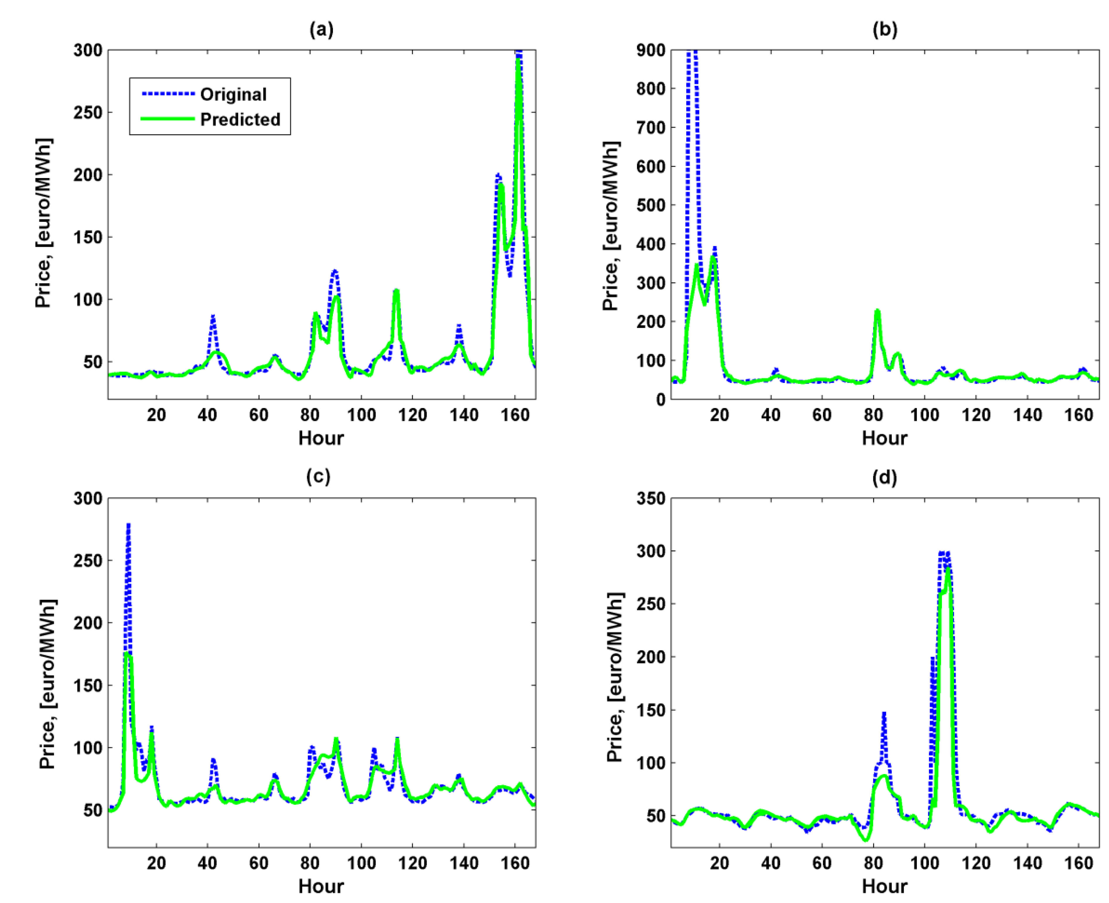
Table 8, occurrence of price spikes generally existing in the winter period is predicted by the proposed methodology with high accuracy and confidence. In this context, price spike prediction can be considered as a forecasting of a price volatility rather than exact price value. In order to graphically illustrate the price forecast performance of the proposed methodology and emphasize its ability to capture spikes, the forecasted and actual signals for the four selected spiky weeks (1,2,5 and 28 in
Table 8) of the Finnish day-ahead energy market of year 2010 are shown in
Figure 6.
Table 8.
Obtained results from the proposed forecasting methodology for each week of 2010.
Table 8.
Obtained results from the proposed forecasting methodology for each week of 2010.
| Week | 1 | 2 | 3 | 4 | 5 | 6 |
| AMAPE | 9.41 | 25.16 | 6.31 | 5.75 | 7.24 | 4.51 |
| Nsp/Ncorr/Nas_sp | 23/21/22 | 22/22/22 | 0/0/0 | 9/8/8 | 7/7/7 | 1/0/0 |
| Accur./Conf. | 91.30/95.45 | 100/100 | - | 88.89/100 | 100/100 | 0/- |
| Week | 7 | 8 | 9 | 10 | 11 | 12 |
| AMAPE | 6.59 | 30.75 | 6.49 | 6.11 | 4.76 | 3.55 |
| Nsp/Ncorr/Nas_sp | 5/5/5 | 44/39/39 | 2/2/2 | 0/0/0 | 0/0/1 | 0/0/1 |
| Accur./Conf. | 100/100 | 77.27/97.14 | 100/100 | - | -/0 | - |
| Week | 13 | 14 | 15 | 16 | 17 | 18 |
| AMAPE | 2.84 | 2.99 | 3.31 | 5.07 | 6.11 | 6.88 |
| Nsp/Ncorr/Nas_sp | 0/0/0 | 0/0/0 | 0/0/0 | 0/0/0 | 0/0/0 | 0/0/0 |
| Accur./Conf. | - | - | - | - | - | - |
| Week | 19 | 20 | 21 | 22 | 23 | 24 |
| AMAPE | 7.43 | 15.51 | 6.35 | 8.03 | 7.23 | 6.46 |
| Nsp/Ncorr/Nas_sp | 0/0/0 | 0/0/0 | 0/0/0 | 0/0/0 | 0/0/0 | 0/0/0 |
| Accur./Conf. | - | - | - | - | - | - |
| Week | 25 | 26 | 27 | 28 | 29 | 30 |
| AMAPE | 6.15 | 7.23 | 4.26 | 12.82 | 4.56 | 5.38 |
| Nsp/Ncorr/Nas_sp | 0/0/0 | 0/0/0 | 0/0/0 | 9/7/7 | 0/0/2 | 0/0/0 |
| Accur./Conf. | - | - | - | 77.78/100 | -/0 | - |
| Week | 31 | 32 | 33 | 34 | 35 | 36 |
| AMAPE | 7.58 | 6.34 | 3.06 | 3.14 | 4.99 | 2.19 |
| Nsp/Ncorr/Nas_sp | 0/0/0 | 0/0/0 | 0/0/0 | 0/0/0 | 0/0/0 | 0/0/0 |
| Accur./Conf. | - | - | - | - | - | - |
| Week | 37 | 38 | 39 | 40 | 41 | 42 |
| AMAPE | 3.64 | 2.65 | 3.64 | 2.43 | 3.83 | 4.09 |
| Nsp/Ncorr/Nas_sp | 0/0/0 | 0/0/0 | 0/0/0 | 0/0/0 | 0/0/0 | 0/0/0 |
| Accur./Conf. | - | - | - | - | - | - |
| Week | 43 | 44 | 45 | 46 | 47 | 48 |
| AMAPE | 5.91 | 3.14 | 2.26 | 2.83 | 4.03 | 17.12 |
| Nsp/Ncorr/Nas_sp | 0/0/1 | 0/0/0 | 0/0/0 | 0/0/0 | 0/0/0 | 12/7/8 |
| Accur./Conf. | - | - | - | - | - | 58.33/87.50 |
| Week | 49 | 50 | 51 | 52 | | |
| AMAPE | 8.37 | 11.02 | 5.70 | 4.22 | | |
| Nsp/Ncorr/Nas_sp | 3/3/3 | 35/33/34 | 9/8/11 | 0/0/1 | | |
| Accur./Conf. | 100/100 | 82.86/96.67 | 88.89/72.73 | -/0 | | |
As can be seen in
Figure 6, all the forecasted price curves acceptably follow the actual curves. The proposed methodology based on a hybrid iterative strategy is able to capture essential features of the given price time series: non-constant mean, cyclicality, exhibiting daily and weekly patterns, major volatility and significant outliers. This ability results in the superiority of the proposed methodology over all the examined alternative techniques.
Figure 6.
Real and predicted prices for the four weeks with prominent spikes of the Finnish energy market of year 2010: (a) Week 1; (b) Week 2; (c) Week 5; (d) Week 28.
Figure 6.
Real and predicted prices for the four weeks with prominent spikes of the Finnish energy market of year 2010: (a) Week 1; (b) Week 2; (c) Week 5; (d) Week 28.
The total running time to set up the proposed separate forecasting strategy including its normal price module, price spike module, and iterative prediction process for the first forecast day is about 42 h since price predictions produced by the initial forecasting model are required over the period up to 365 days. The running time of the training and prediction procedures for the next forecast days after the first one is significantly lower (about 50 min) and considered suitable for day-ahead energy market operation. All the competitive non-separate forecasting approaches examined for price prediction have lower computation costs than the proposed separate forecasting strategy but are outperformed by the proposed strategy in terms of forecasting accuracy. The prediction accuracy is a crucial concern for a forecasting method (as far as the computation time is reasonable). The PNN and RVM classifiers of the compound classifier have relatively lower computational costs than the alternative back-propagation NN and SVM, respectively. The training process of the PNN is carried out through one run of each training sample unlike the back-propagation algorithm. The RVM is faster than the SVM in decision speed, as the RVM has a much sparser structure (the number of relevant vectors versus the number of support vectors). The computation times to set up the proposed and competitive forecasting strategies are measured on a hardware platform comprising an Intel Core i5 2.40 GHz processor (Intel Corporation, Santa Clara, CA, USA) and 3.24 GB RAM. All computer codes are provided by the MATLAB (MathWorks, Natick, MA, USA) and R (R Development Core Team, Auckland, New Zealand) software packages.

