1. Introduction
Renewable energy sources (RESs), with powers varying from 100 kW to a few MW, are increasingly present in electrical networks. The economic opportunities, the liberalization and the potential benefits for electrical utilities (peak shaving, support for distribution and transmission networks) are contributing to the already existing trend, leading to a more decentralized energy market [
1]. The RES systems can be used in small, decentralized power plants or in large ones, they can be built with small capacities and can be used in different locations. In isolated areas where the cost of the extension of the power systems (from the utilities’ point of view) or the cost for interconnection with the grid (from the customer’s point of view) are very high with respect to the cost of the RES system, these renewable sources are suitable. The RES systems are “environmentally friendly” and appropriate for a large series of applications, such as stand-alone systems for isolated buildings or large interconnected networks. The modularity of these systems make possible their expansion in the case of a subsequent load growth.
As RESs becomes more reliable and economically feasible, there is a trend to interconnect RES units to the existing utilities to serve different purposes and offer more possibilities to end-users, such as:
- a.
Improving availability and reliability of electric power;
- b.
Peak load shaving;
- c.
Selling power back to utilities or other users;
- d.
Power quality (improvement of the voltage level, without an additional regulation of reactive power).
The increasing penetration rate of RES in the power systems is raising technical problems, as voltage regulation, network protection coordination, loss of mains detection, and RES operation following disturbances on the distribution network [
2]. These problems must be quickly solved in order to fully exploit the opportunities and benefits offered by the RES technologies. As the RES are interconnected to the existing distribution system, the utility network is required to make use of RES maintaining and improving the supply continuity and power quality delivered to the customers [
3].
The present paper deals with the experimental investigation of the impact of renewable sources on power quality. The voltage fluctuations generated by wind turbines are analyzed, during continuous operation as well as for generator interconnection. The steady state voltage variation at the point of common coupling due to the PV system connection is analyzed for sunny and cloudy days. The PV systems interfaced to the main grid with the help of inverters are injecting harmonics in the 50 Hz grid. The correlation between the PV generated power and the main harmonic distortion indices is presented.
In particular, in
Section 2, the power quality in distributed generation systems is discussed.
Section 3 is devoted to the voltage fluctuations determined by a 0.65 MVA wind turbine. In
Section 4, the investigation of steady state voltage variations at the point of common coupling is carried out. Current harmonics injected in the 50 Hz grid are experimentally illustrated in
Section 5. Finally, conclusions are given in
Section 6.
3. Voltage Fluctuations (Flicker Effect)
The possibility for reducing voltage fluctuations determined by wind turbines requires the establishment of some regulations, when and how often the wind turbines operators can start or vary the output power. In some cases, voltage fluctuations problems can be solved without a detailed study, by simply adjusting a control element, until the voltage flicker level is reduced below the standardized value [
7,
8]. In some other cases, complex analysis limiting flicker is requested. Determination of voltage fluctuations due to output power variations of renewable sources is difficult, because they depend on the source’s type, generator’s characteristics and network impedance.
For the case of wind turbines, the long term flicker coefficient
Plt due to commutations, computed over a 120 min interval and for step variations, is given by Equation (1) [
9]:
where
N120 is the number of possible commutations in a 120 min interval,
kf(ψ
sc) is the flicker factor defined for angle ψ
sc = arctan(
Xsc/Rsc),
Xsc is the reactance of short-circuit network impedance,
Rsc is the resistance of short-circuit network impedance
Sr is the rated power of the installation, and
Ssc is the fault level at point of common coupling (PCC). In the present paper, the power system, where the wind far is connected, is simulated through
Ssc and ψ
sc. The propagation of perturbations within the electrical network is not investigated.
For a 10 min interval, the short-term flicker
Pst is defined by Equation (2) [
9]:
where
N10 is the number of possible commutations in a 10 min interval.
The values of flicker indicator for wind turbines, due to normal operation, can be evaluated using flicker coefficient
c(ψ
sc, υ
a), dependent on average annual wind speed, υ
a, in the point where the wind turbine is installed, and the phase angle of short circuit impedance, ψ
sc:
The flicker coefficient
c(ψ
sc, υ
a) for a specified value of the angle ψ
sc, for a specified value of the wind speed υ
a and for a certain installation is given by the installation manufacturer, or can be determined experimentally based on standard procedures. Depending on the voltage level where the wind generator (wind farms) is connected, the angle ψ
sc can take values between 30° (for the medium voltage network) and 85° (for the high voltage network). Flicker evaluation is based on the IEC standard 61000-3-7 [
8], which provides guidelines for emission limits for fluctuating loads in medium and high voltage networks.
Table 1 lists the recommended values.
Table 1.
Flicker planning levels for medium voltage (MV) and high voltage (HV) networks.
Table 1.
Flicker planning levels for medium voltage (MV) and high voltage (HV) networks.
| Flicker severity factor | Planning levels |
| MV | HV |
| Pst | 0.9 | 0.8 |
| Plt | 0.7 | 0.6 |
The flicker evaluation determined by a wind turbine of 0.65 MVA is analyzed. The wind turbine has a tower height of 80 m, the rotor diameter is 47 m, and the swept area is 1,735 m
2. The electrical energy production during the months of February and March were 127,095 kWh and 192,782 kWh, respectively. The average wind speed, measured at 60 m height, during February was 6.37 m/s, while during March it was 7.32 m/s. The measurement data for the month of February are reported in
Table 2. The experimental data for the month of March are reported in
Table 3.
Table 2.
Wind turbine experimental data during the month of February.
Table 2.
Wind turbine experimental data during the month of February.
| Average wind speed at hub height (m/s) |
|---|
| 60 m | 50 m | 40 m |
| 6.37 | 6.30 | 6.045 |
Table 3.
Wind turbine experimental data during the month of March.
Table 3.
Wind turbine experimental data during the month of March.
| Average wind speed at hub height (m/s) |
|---|
| 60 m | 50 m | 40 m |
| 7.32 | 7.165 | 6.95 |
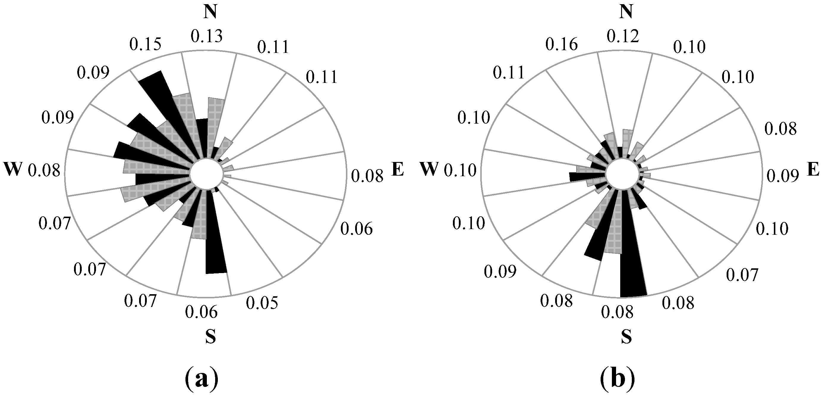
The wind rose graph presented in
Figure 1 illustrates the percent time and percent energy in each direction sector. The wind rose is divided in 16 sectors, each one of 22.5°. The outer circle represents 30% of the total energy or time. The black areas represent the percent of total wind energy, and the shaded areas illustrate the percent of total time. The outer values represent the intensity of wind turbulence in the investigated location. The turbulence intensity σ
0 is defined as the ratio between the standard deviation σ
v of wind speed and the average wind speed in a specified time interval. In the case of reduced wind speeds, high turbulence intensities can lead to an increase of the produced power. In practice, for the nominal wind speed, large turbulence intensities can reduce the produced power as the control systems difficulty follow the sudden and large wind speed variations.
Figure 1a illustrates the wind rose, at 60 m height, of the wind turbine during February. As it can be seen, the prevailing winds in this area come from the west, south and northwest.
Figure 1b illustrates the wind rose, at 60 m height, of the wind turbine during March. As it can be seen, the prevailing winds in this area come from the west, south and southwest.
Figure 1.
Wind rose for (a) the month of February and (b) for the month of March.
Figure 1.
Wind rose for (a) the month of February and (b) for the month of March.
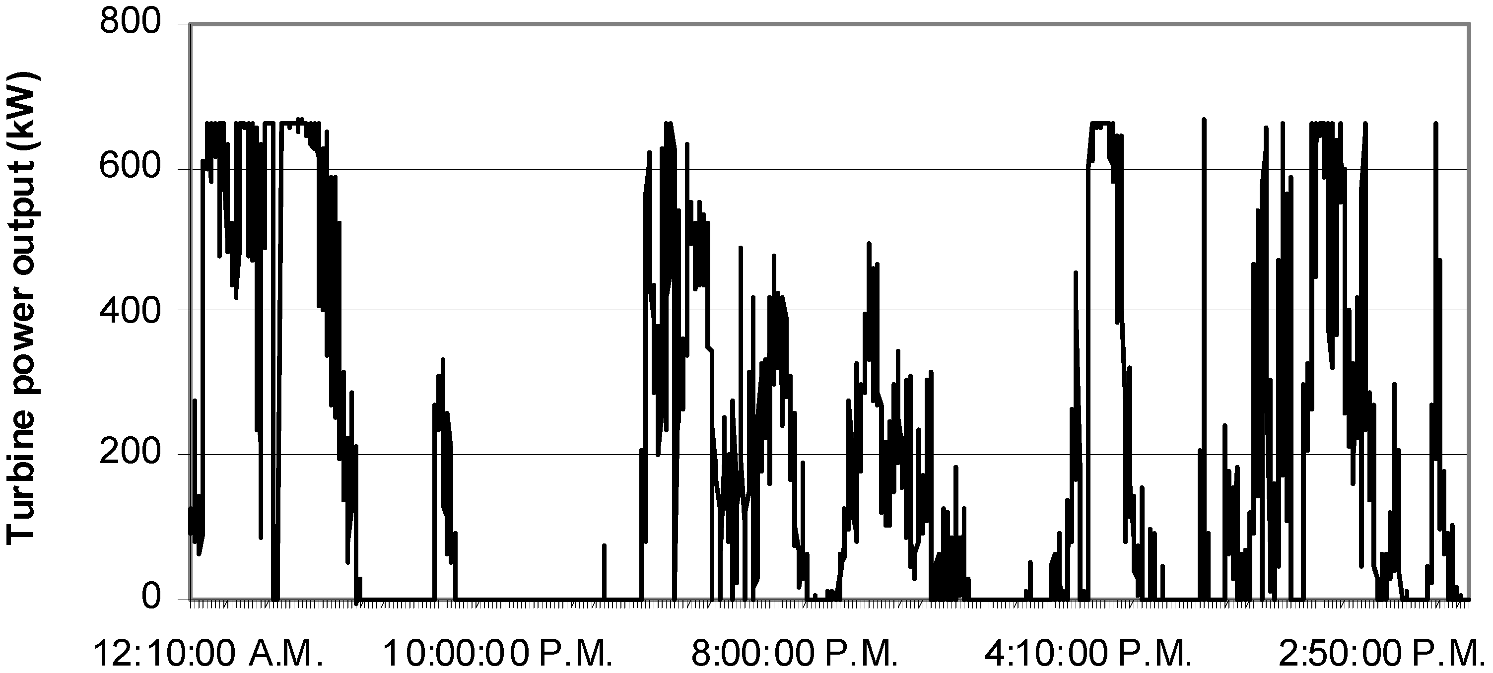
Measurements were conducted on the wind turbine system described in this paper. The variation of wind speed over the monitoring period is shown in
Figure 2. The variation of turbine output power is shown in
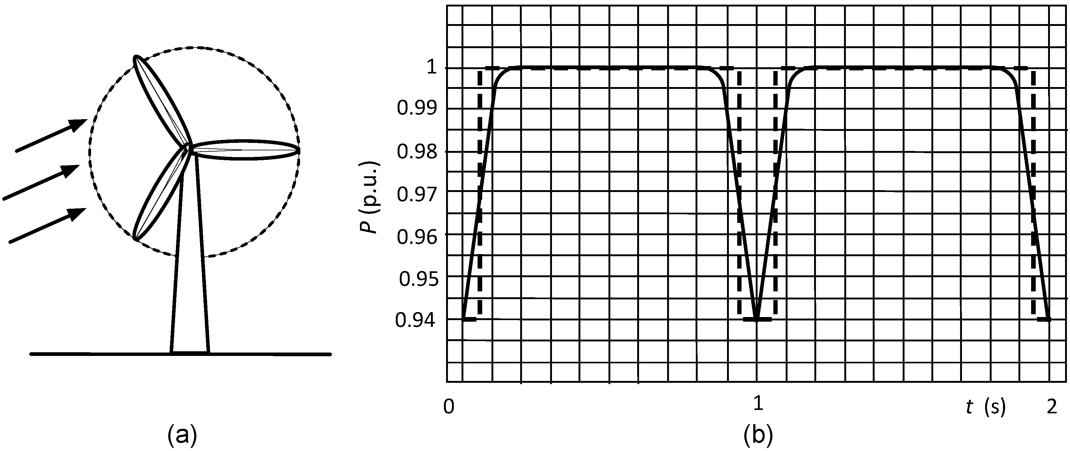
Figure 3. The intermittent character of the produced power is clearly visible. The tower shadow effect for the wind generator determines a variation of the absorbed energy, which is measured as a power variation at generator terminals.
Figure 4a shows the wind generator, while
Figure 4b illustrates the tower shadow effect corresponding variation of the generator output power.
Figure 2.
Wind speed variation during the one month monitoring period.
Figure 2.
Wind speed variation during the one month monitoring period.
Figure 3.
Turbine output power variation during the one month monitoring period.
Figure 3.
Turbine output power variation during the one month monitoring period.
Figure 4.
Tower shadow effect: (a) wind generator and (b) output power variation.
Figure 4.
Tower shadow effect: (a) wind generator and (b) output power variation.
The measured values of the flicker coefficient
c(ψ
sc, υ
a) for different values of the annual average wind speed υ
a and for different network impedance angle ψ
sc are reported in
Table 4.
Table 5 gives the flicker coefficient
kf values for voltage step variations, for the same wind generator.
Table 4.
Values of the flicker factor for various values of the wind speed va and for various angles ψsc.
Table 4.
Values of the flicker factor for various values of the wind speed va and for various angles ψsc.
| Annual wind speed
va (m/s) | Network impedance angle ψsc (°) |
|---|
| 30° | 50° | 70° | 85° |
|---|
| 6 | 3.1 | 2.9 | 3.6 | 4.0 |
| 7.5 | 3.1 | 3.0 | 3.8 | 4.2 |
| 8.5 | 3.1 | 3.0 | 3.8 | 4.2 |
| 10 | 3.1 | 3.1 | 3.8 | 4.2 |
Table 5.
Values of the flicker factor kf.
Table 5.
Values of the flicker factor kf.
| Conditions of operation | Network impedance angle ψsc (°) |
|---|
| 30° | 50° | 70° | 85° |
|---|
| Flicker factor kf for voltage step variations | With start at minimum speed | 0.02 | 0.02 | 0.01 | 0.01 |
| With start at rated speed | 0.12 | 0.09 | 0.06 | 0.06 |
The computations based on the values reported in
Table 4 and
Table 5 lead to the flicker indicator values:
Continuous operation, annual average wind speed υ
a = 7.5, interconnection with the medium voltage network (ψ
sc = 50°,
Ssc = 300 MVA,
Sr = 0.65 MVA), given by Equation (4):
Generator interconnection at minimum speed of the wind turbine, given by Equation (5):
Generator interconnection at rated speed of the wind turbine, given by Equation (6):
Due to the output power variations of the wind turbines, voltage fluctuations are produced. Voltage fluctuations are produced due to the wind turbine switching operations (start or stop), and due to the continuous operation. The presented voltage fluctuations study, made for one turbine, becomes necessary in large wind farms as the wind power penetration level increases quickly.
4. Steady State Voltage Variations
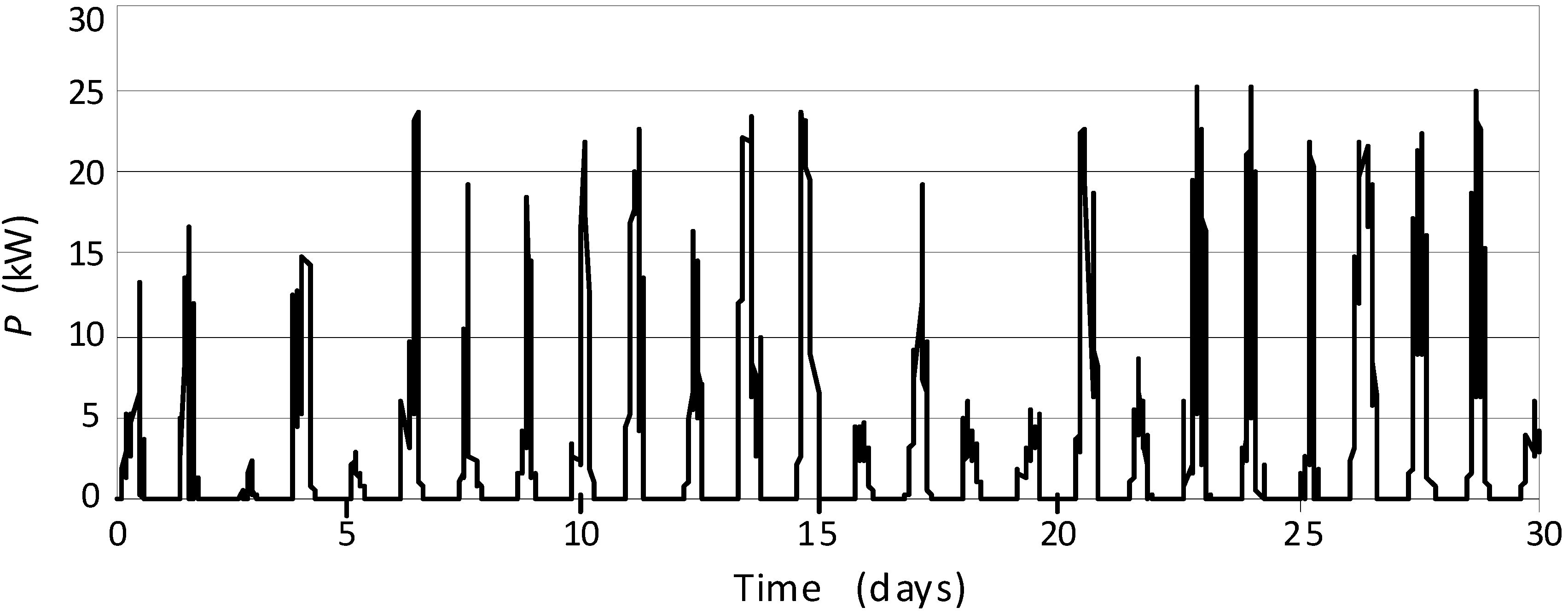
The variable nature of solar radiation, the weather changes or passing clouds can cause variations of PV output power [
10]. The variation of the power produced by a 30 kW PV system is illustrated in
Figure 5.
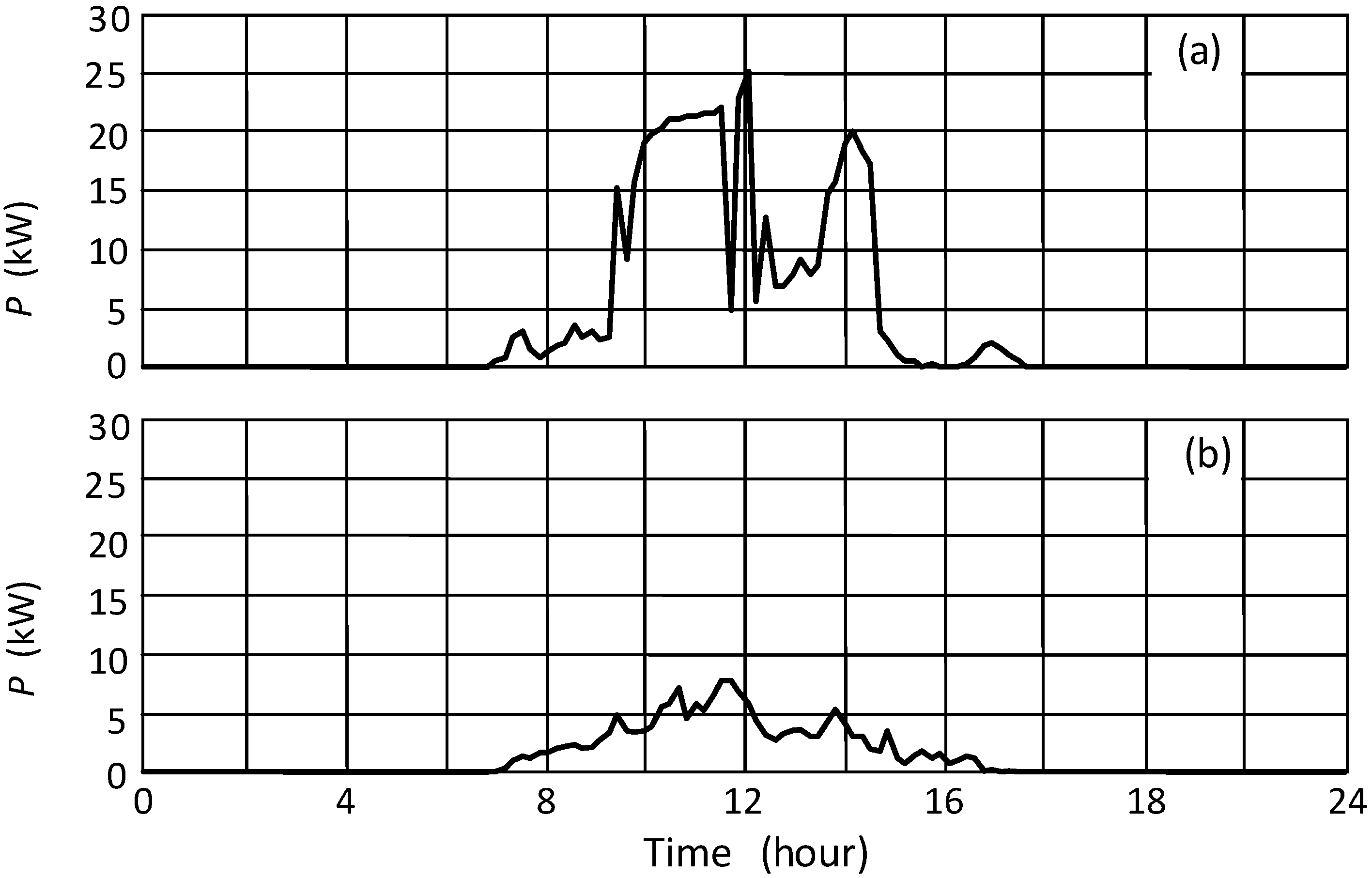
Figure 6a shows the generation power in a sunny day, while
Figure 6b illustrates the generation power in a cloudy day. Typically, the photovoltaic panels installed on house roves generate up to 5 kW. The sources are normally connected through a single-phase inverter to the low voltage supply system [
11].
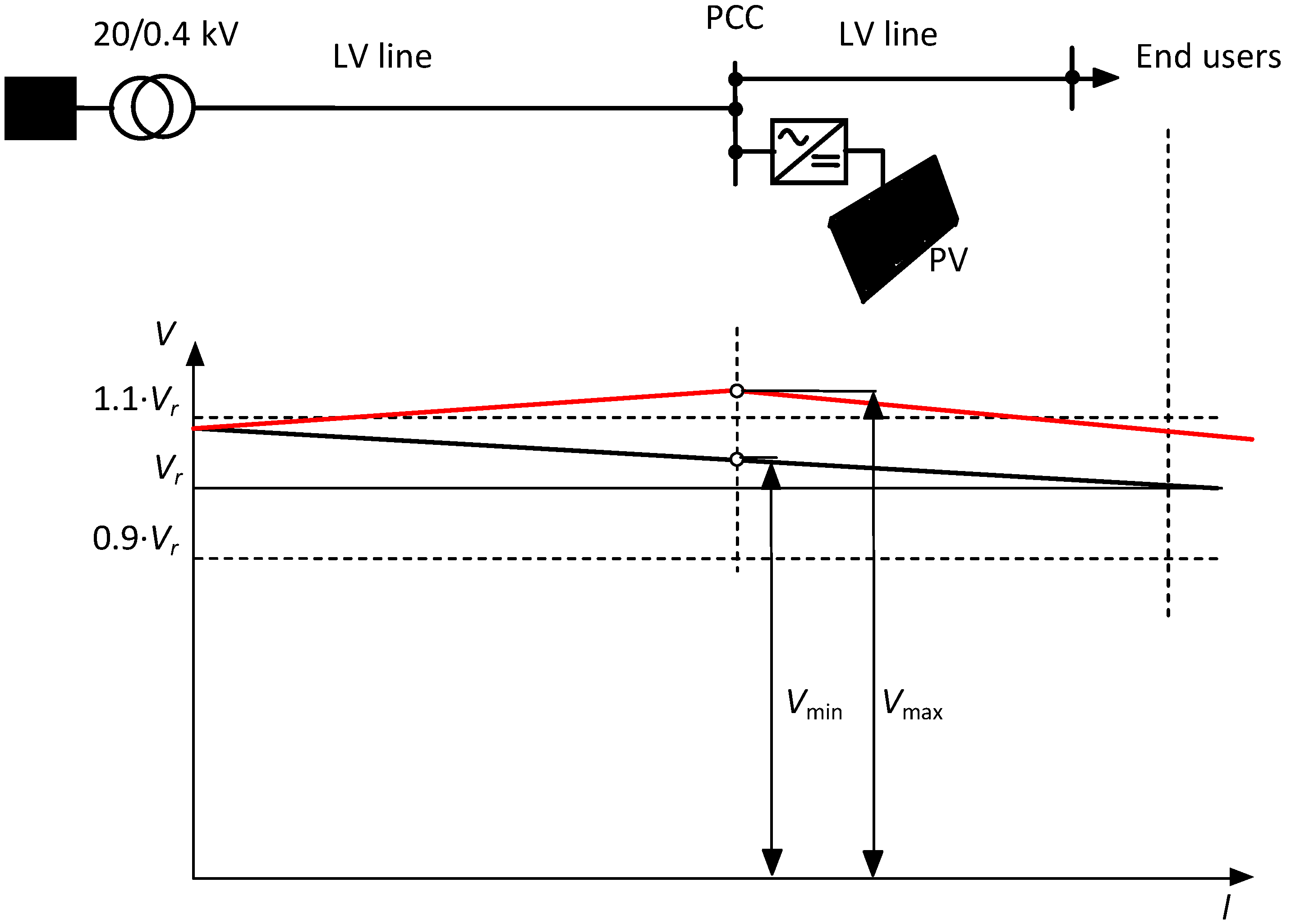
The connection of these variable renewable sources can cause a voltage rise at PCC and in the grid. The utility has the general obligation to ensure that customer voltages are kept within prescribed limits. A voltage variation Δ
V between
Vmax and
Vmin, can appear on short periods. This voltage variation can highly stress the electrical devices supplied by the power system, and in particular the owner of the photovoltaic facility (as shown in
Figure 7).
Figure 7 illustrates the possible case of a summer mid-day, when the load downstream PCC is relatively small and the PV output power exceeds the demand.
Figure 5.
Variation of PV system power output during a month.
Figure 5.
Variation of PV system power output during a month.
Figure 6.
Variation of PV system power output during: (a) sunny day and (b) cloudy day.
Figure 6.
Variation of PV system power output during: (a) sunny day and (b) cloudy day.
Figure 7.
Influence of PV on voltage level: without PV source generating (black line); with PV source generating (red line).
Figure 7.
Influence of PV on voltage level: without PV source generating (black line); with PV source generating (red line).
The voltage variations can affect the characteristics of the electrical equipment and household appliances (loss of the guaranteed performances, modifications of the efficiency) leading in some cases even to the interruption of operation [
12]. The voltage variation at PCC can be expressed as:
where
SPV is the power produced by PV,
Ssc is the short circuit power at PCC, ψ
sc = arctan(X/R) is the angle of the network short circuit impedance, φ is the phase angle of the PV output current (we consider that the electric quantities are sinusoidal) [
12]. In existing power systems, there are measures such that the line voltage to be sinusoidal. In Equation (7), the system harmonics are not considered.
The analysis of Equation (7) highlights that limiting the voltage variation ΔV requires a careful analysis of the grid where the PV installation is connected. A power system characterized by a high short-circuit current (high short-circuit power) and a small angle ψ will be characterized by reduced voltage variations at PCC. For the medium voltage network (ψ 50°) and the low voltage network (ψ 30°), with small short-circuit powers, especially if the PCC is far from the substation point, large voltage variations may occur caused by PV installation of large capacity.
At low and medium voltage levels, the utilities have established limits for the amplitude of the voltage variations, which must not be exceeded during normal operation. Due to the statistical nature of the steady state voltage variations, the EN 50160 standard stipulates statistical limits [
7]. In some countries the limit ±10% established in EN 50160 is applied, while other current guidelines, elaborated in different countries, impose more restrictive limits for the voltage variations both for the light load as well as for the heavy load conditions, e.g., ±6% [
13]. The relevant variations of the voltage will overlap the voltage’s variations caused by load modification and can lead to the widening of the voltage admissible bands.
5. Current Harmonic Perturbations
In order to connect PV power systems with the grid, an inverter that transforms the DC output power of the PV to the 50 Hz AC power is required. The large scale PV systems are interconnected to the main grid with pulse width modulated three-phase inverters [
14]. These inverters, equipped with a grid-side filter, have a small harmonic contribution (the total current harmonic distortion,
THDI, is small), and thus the influence on voltage waveform at PCC is negligible. The small capacity PV systems are interconnected to the main grid with the help of simple single-phase inverters, which can cause important current harmonics. General requirements can be found in standards, especially those for the interconnection of distributed generation systems to the grid and for photovoltaic systems [
1,
15]. In the standard IEEE 1547, the harmonic current injection of PV at the PCC must not exceed the limits stated in
Table 6.
Table 6.
Main parameters for the PV system used in the simulation.
Table 6.
Main parameters for the PV system used in the simulation.
| Individual harmonic order | h < 11 | 11 ≤ h < 17 | 17 ≤ h < 23 | 23 ≤ h < 35 | 35 ≤ h | TDD |
|---|
| Percent (%) | 4 | 2 | 1.5 | 0.6 | 0.3 | 5 |
The harmonic spectrum is a function of inverter topology, switching frequency, control, etc. The measurements were conducted for a particular case of a photovoltaic plant connected to the main supply through a 6-pulse converter. The influence of converter configuration on harmonic spectrum was not analyzed. The experimental measurements reveal high values, but not relevant, of THDI. The establishment of an indicator that better illustrates the perturbations at PCC, during the operation period of renewable sources, is proposed. The function of photovoltaic systems is accompanied by the injection of some harmonic perturbation into the grid, with a total harmonic distortion factor dependent on the generated power.
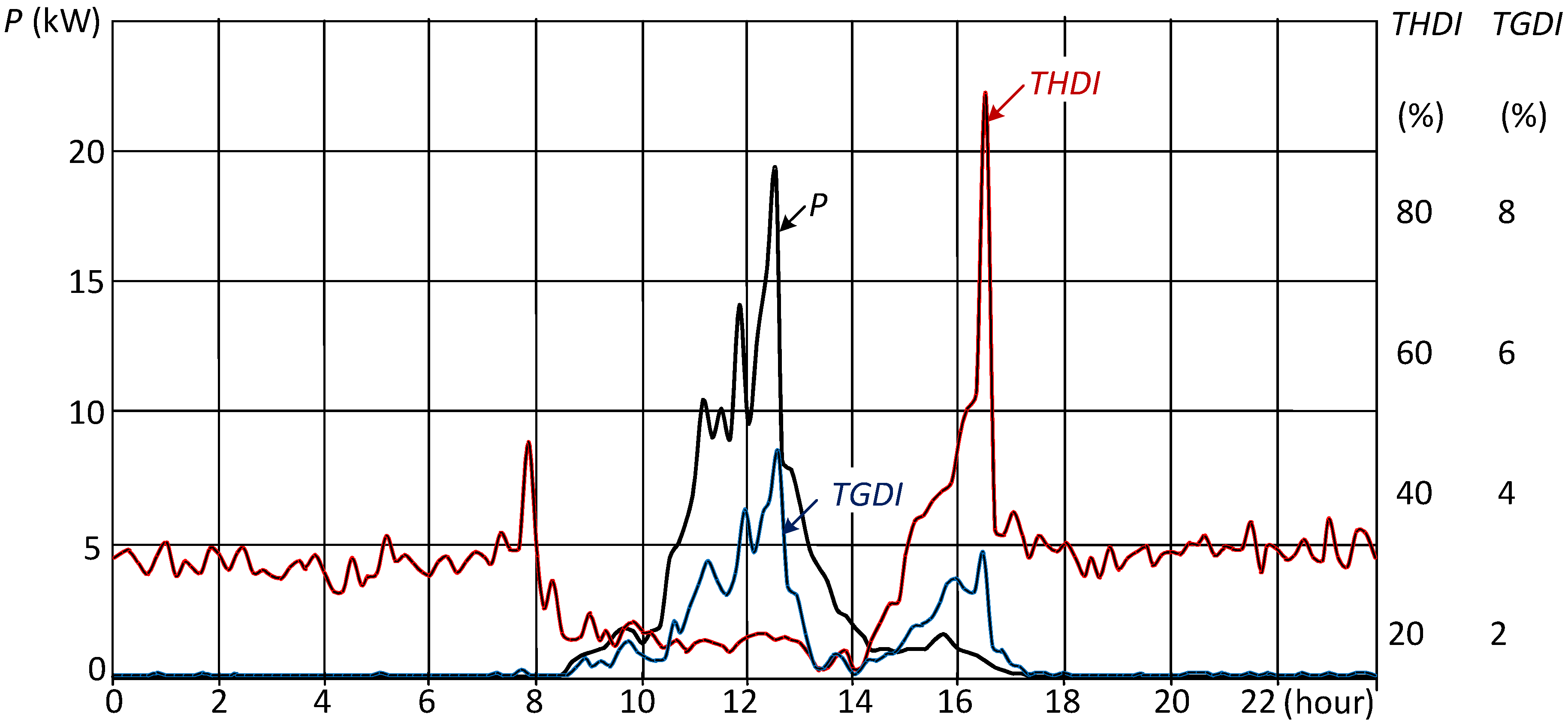
Figure 8 illustrates the correlation between the generated power and total current harmonic distortion factor
THDI, for one monitored day (the 6th day of the monitoring period shown in
Figure 5). The analysis of the total harmonic distortion factor has to consider that, for high variability installations, the large
THDI values can lead to inappropriate conclusions. The total harmonic factor is related to the fundamental component of the electric current
I1:
For the periods with low irradiation (especially during the morning and evening periods), the electric current injected into the grid presents a reduced fundamental component, resulting in a high distortion factor. As the electrical current has small values, the voltage drops in the power system are negligible, and thus the voltage waveform at PCC is not affected.
For assessing the operation of PV installations in terms of harmonic disturbances injected at PCC, the use of a new indicator
Total Generator Distortion Index (
TGDI) is proposed. This indicator is useful for high variability sources, which is related to the rated fundamental current of photovoltaic system
Ir:
where the rated current
Ir is established and indicated for pure sinusoidal measures (a constant current value of the installation).
Figure 8.
Correlation between the generated power, the total current harmonic distortion factor THDI and the total generator distortion index TGDI.
Figure 8.
Correlation between the generated power, the total current harmonic distortion factor THDI and the total generator distortion index TGDI.
The relation between TGDI and THDI can be expressed as:
We consider that the rated current
Ir, established by the plant manufacturer, has a constant value for pure sinusoidal measures; the current
I is the measured electrical current (inclusive all harmonics). In this paper, it is considered that harmonics are determined by converter at the interconnection point with the main supply. When the generated power is high (large value of RMS electrical current), the fundamental current is high and the
THDI is small [
16,
17]. For small generated powers, the fundamental current is small and the
THDI is high. From a practical point of view, this fact is not highly important as the small current values do not influence the voltage quality at point of common coupling. The analysis of waveforms illustrated in
Figure 8 shows that the indicator
TGDI better defines the effect of harmonics into the power grid, with a variation corresponding to the power injected into the network and which determines the voltage waveform at PCC, without transmitting insignificant information for the periods with very low generation. The
THDI values were measured for a winter day, while the
TGDI values were computed based on the conducted measurements.
The interconnection of the PV system to the main grid must not determine the total harmonic factor to exceed the stipulated values, which can occur especially when the PV system is generating the maximum power output.


