1. Introduction
The issue of energy efficiency in the building sector is at the centre of the energy policies of the European Union. The Green Paper “Towards a European Strategy for the Security of Energy Supply” [
1] estimated that the residential and tertiary sector, the major part of which is composed of buildings, accounts for more than 40% of final energy consumption in the Community and is in expansion, a trend which is bound to increase its energy consumption and hence also its carbon dioxide emissions.
Energy policies will cover both new buildings and existing buildings. The European Directive 2002/91/EC [
2], known as Energy Performance Building Directive (EPBD) highlights the fact that buildings will have an impact on long-term energy consumption and new buildings should therefore meet minimum energy performance requirements, tailored to the local climate. The transposition of the above mentioned Directive in the Member States, generated new regulations and laws aimed to significantly increase the energy performances of new constructions. The more recent Directive 2010/31/EC [
3] goes further, in terms of energy performances for buildings: by 31 December 2020, all new buildings must be nearly zero-energy buildings; and after 31 December 2018, new buildings occupied and owned by public authorities must be nearly zero-energy buildings.
The more recent European Directive 2012/27/UE [
4] establishes a common framework of measures for the promotion of energy efficiency within the Union in order to ensure the achievement of the Union’s 2020 20% headline target on energy efficiency and to pave the way for further energy improvement beyond that date.
The contents of the European directives, which must be transposed and applied by the Member States through local legislation, consider both new buildings and those of the existing building stock, which are the real problem. The energy performance of existing buildings, as stated before, is very low and an energy policy that focuses on turn-over (i.e., replacement of existing buildings with new buildings) is not realistic since this process would take far too many years.
Additionally, although the potential in terms of primary energy reduction in existing buildings is relatively high, being more than 20%, the problems to be faced in carrying out actions on a large scale are many:
- -
each building has different characteristics and therefore requires a careful analysis of the retrofit measures that can be taken in relation to the construction technologies, plant characteristics, methods of use, but also to the climatic conditions;
- -
it is not so easy to acquire a good understanding of facility energy use;
- -
the market offers a wide range of possible technologies to improve the energy efficiency of buildings and related facilities, to take advantage of renewable energy sources and to improve the management: the choice may be difficult owing to lack of appropriate skills;
- -
the economic aspects should not be underestimated, since the retrofit, without financial support, may require considerable investments which may moreover have long payback times.
Actions to improve the energy performance of buildings cannot be improvised, but must be defined considering awareness, professional skills and, above all, an effective methodological approach [
5].
Before identifying the retrofits that can be applied in existing buildings in order to increase their energy performance, and before planning strategies, it is essential to know the energy quality of building components and building systems: energy audit procedures are the tools that allow the achievement of this goal.
Amongst the energy audit procedures, the infrared audit is an interesting tool for its intrinsic characteristics. Sarto and Martucci in [
6] deal with this issue analysing both theoretical aspects and application aspects.
Thermographic survey techniques, through the use of infrared cameras, are not a recent development. There are really two essential elements for achieving a good infrared audit: a high performance instrument and the technical skill of the infrared auditor. Thermographic analysis is very useful for evaluating a building’s energy performance, both for its envelope and its facilities. In fact it could lead to identification of many energy problems such as bad final design, construction, installation or building malfunctions. For example, the knowledge of structural and energy performance of existing buildings could render feasible their respective retrofitting activities, while in new buildings it is possible to check the accuracy of the “as-built” construction compared to the project details. It is also used to verify the presence of air seepage, moisture or water leaks.
In order to correctly define the performance of a building envelope, it is very important to know, in addition to the characteristics of the building materials, the reflected ambient temperature as well as the weather conditions (outside temperature trend, relative humidity, rainfall intensity, wind direction and velocity, solar radiation, etc.).
The subject of the application of the thermographic technique in the building sector for diagnostic purposes has prompted several research studies in order to verify not only the potential but also the critical aspects of this interesting technique.
Studies have often addressed issues such as the calculation of the emissivity or transmittance, but under stationary conditions and often through laboratory tests. Our study aims to carry out a quantitative analysis and not qualitative, starting from the reading of the IR thermographic images.
Fokaides and Kalogirou [
7] presented a study to calculate the overall heat transfer coefficient (U-value) in building envelopes starting from infrared thermography (IR). The U-values obtained are validated by means of measurements performed with the use of a thermo-hygrometer for two seasons (summer and winter), as well as with the notional results provided by the relevant EN standard, and finally with the use of heat flux meters. The percentage absolute deviation between the notional and the measured U-values for IR thermography is found to be at an acceptable level, being in the range of 10%–20%. The paper also discusses the applicability of the method due to the non-steady heat transfer phenomena observed at and in building shells. According to our analysis, finally one can observe that the sensitivity analysis is a great advantage of using IR system, in that in IR thermography results can be corrected considering radiation effects and this only requires a fairly short and reliable procedure. The analysis was conducted from inside the building, so it was possible to simplify some of the parameters required for the calculation of the U-value. On the other hand for studies conducted on the outside, the value of the external convective coefficient cannot be considered constant, and must also be calculated on the basis of weather conditions (wind speed, air temperature variation,
etc.) to achieve an acceptable result.
The objective of the study presented by Hoyano, Asano and Kanamaru [
8] is to calculate the sensible heat flux from the exterior surface of buildings using time sequential thermography, based upon an appropriate simplification of the building model. In particular, the authors calculated the temperature distribution on the surface of two representative buildings using a thermal infrared camera. During the survey both the exterior surface temperature at three points throughout the day (before sunrise, at noon and after sunset) and the weather and other related conditions (air temperature, horizontal-plane global solar radiation and wind velocity) were all monitored. Then the authors analysed the thermographs, dividing them into zones by constructing polygons and according to temperature, shape, material and position. Thus the surface temperatures in each polygon were measured and averaged to obtain the surface temperature of each zone. Starting from the surface temperature and their area (calculated from the blueprints), it is possible to calculate the sensible heat flux but not the U-value, while the local heat conductivity and the air temperature are assumed to be constant for all elements. The study concludes with the remark that, although the convective heat transfer coefficient varies widely at different positions on the surface of a building, there is at present no known method for measuring its spatial distribution.
Haralambopoulos and Paparsenos [
9] wished to define a methodology to determine the level of thermal insulation in old buildings through spot measurements of thermal resistance and planar infrared thermography. In the equation employed for the calculation of the thermal transmittance coefficient they use, as convection heat transfer coefficient for the interior and exterior surfaces of the wall, the value according to the Greek Thermal Insulation Regulation.
Infrared thermography for building diagnostics is the issue of the work of Balaras and Argiriou [
10], who review the main areas for using IR with an emphasis on how it was implemented to support office building audits the TOBUS methodology [
11]. The authors stated that although an IR inspection will increase the time necessary to perform a building audit, it can provide some very useful information.
The infrared audit applied to the evaluation of the energy performance of the building envelope of existing buildings from outside, discussed in this paper, presents many advantages. With this diagnostic technique it is possible to thermally map the surfaces of the external walls from the outside, thus without disturbing the occupants, and very quickly. The latest generation of thermal imagers is able to return mappings with a high level of definition, a higher level of accuracy and images can also be processed later.
This technique of investigation, therefore, it is very suited to performing a thermal mapping of a large number of buildings. It is an “infrared screening” that can provide useful information to local Administrations, for example Municipalities, to carry out approximate assessments of the energy quality of existing buildings or to make preliminary checks on the application of the rules and regulations (for instance check if the heating systems are activated during the hours in which this is permitted).
The issue of the infrared scanning was presented and discussed by Dall’O’
et al. [
12] in a study aimed at an extensive application of the thermography on 87 public buildings (mainly school buildings). The scope of the work, however, was to conduct a qualitative assessment of the methodology, highlighting, with statistical approach, the application fields.
The objective of this work is different: the purpose is to evaluate whether an application of thermography on a number of existing buildings, which we define as “infrared screening, can provide quantitative information: it allows the determination, indirectly, of a rough estimate of the values of the thermal transmittance (U-values) of the external walls. This type of evaluation is quite complex because the variables involved are many (i.e., weather conditions, outdoor air temperature, indoor air temperature, thermo-physical properties of the wall, mode of use of the systems, the built environment outside, etc.). In the method of analysis two constraints were also placed: the need to make the infrared audit in a short time and uncertainty about the exact conditions inside the buildings investigated, about which we know only that they are heated.
The infrared audit campaign was carried out in January 2013, on 14 existing residential buildings located in Milan Province (Italy) made in different construction periods and characterised, therefore, by different building technologies and by different energy performances. In order to evaluate the results, the U-values obtained indirectly through the thermography of the opaque walls, were compared with the actual known values in order to verify the reliability of the method and the possible margin of error. The results of the field testing, presented and discussed later, permitted the testing of an expeditious method of diagnosis and the assessment of areas of application within which acceptable results are provided.
3. Theoretical Basis for Calculating U-value
In order to calculate the heat flux
ϕ (W/m
2) between two environments separated by a wall, in the steady state conditions, it is possible to use Equation (1) where
Uw (W/m
2 K) is the U-value of the wall and
θin and
θext, expressed in °C, are respectively the internal and the external air temperature:
The heat flux
ϕ can be calculated also as a function of the external heat transfer coefficient
hwe (W/m
2 K) and the difference between the external surface temperature of the wall
θwe and the external air temperature
θext.
combining Equations (1) and (2), it is possible to estimate the U-value of the wall
Uw as a function of the
hew coefficient, the internal air temperature
θin, the external air temperature
θext and the external surface temperature of the wall
θwe.
Knowing the values of the external surface temperature of the wall, derived indirectly from the thermal map, the value of the internal air temperature and the value of the external air temperature, it would then be possible to obtain, in a simple way, the U-value of the wall in question.
This type of evaluation is only theoretical as the heat transmission in reality does not take place in a steady-state condition and the external surface temperature of the wall could be affected by the phenomena of thermal transition due to the thermal inertia. Other factors could render unreliable the values of the thermal map generated by the thermographic survey, for example, the presence of moisture in the wall, radiant heat exchange or the effect of solar radiation.
In our evaluation we are obviously well aware of all these phenomena and try to consider the best arrangement for reducing interpretation errors so that the thermographic technique, although still providing approximate values, has them consistent with the real ones.
The effect due to the presence of moisture is controlled by identifying, in the thermal mapping provided by the infrared camera, an homogeneous area of the wall in which to evaluate the average value of the surface temperature while the effect due to solar radiation is controlled by choosing walls with an orientation that, in the winter season, is not subject to the sunshine. The effect of the non-steady state heat flow condition can be partially reduced by identifying periods in which to perform the measurements with external climatic stability.
From Equation (3) it is possible to observe the significant influence of the convective coefficient
hwe. Its value, in fact, has an effect proportionally to the U-value
Uw. In the standard calculations of the external heat transfer coefficient, pre-calculated values or simple equations are provided by the technical standards, such as the ISO 6946 standard [
14]. In our case we decided to consider the air speed parameter by taking the air velocity from amongst the data of the nearest Regional Agency for Environmental Protection of Lombardia (ARPA) control station, and then to explore this aspect, evaluating the external heat transfer coefficient
hwe in a more analytical manner.
The ISO value, equal to 25 [
14], is a high and precautionary value, because it is used to calculate the heat loss during the design phase of the building envelope. For the purposes of our study, the ISO value will not be used because it does not represent real conditions for which we expected a much lower value.
Figure 1 shows the variation of expected wall-surface temperature difference as a function of transmittance of the wall (U-value) assuming inside outside air temperature difference equal to 20 K. The graph shows data calculated for three different values of
hwe coefficient:
- -
Case A (hwe = 5.8), value obtained from the Jurges equation (see below) with the wind speed equal to 0 m/s;
- -
Case B (hwe = 9.6), for a wind speed of 1 m/s;
- -
Case C (hwe = 25), as defined in ISO 6946 standard, this value is obtained for a wind speed equal to 5 m/s.
Figure 1.
Outside wall-surface temperature difference as a function of U-value of the wall.
Figure 1.
Outside wall-surface temperature difference as a function of U-value of the wall.
We observe that if the hwe value is high, the temperature differences are the smallest obtainable and the order of magnitude of these values is comparable to the margin of error of the measurement instruments, thus not detectable even with high-level instrumentation. Whereas if the coefficient stands at lower values, the temperature difference between the surfaces may be higher, and the possibility of error is reduced.
Despite the use of a FLIR T640bx thermal camera (FLIR Systems Inc., Meer, Belgium), one of the most sophisticated in building field applications, it is observed that the accuracy may be of ±2 °C against temperatures to be collected that differ by little more than one degree, so this detection method is considered inapplicable for the purposes of our study.
3.1. Calculation of Convective Coefficient
We calculate the convective coefficient in actual weather conditions observed during the survey with two methodologies.
The first method requires the application a simplified method to calculate the convective coefficient, the Jurges equation [
13]. The Jurges equation is given by:
where
hwe is convective heat transfer coefficient; and
v is wind velocity near the building element. Anyway, as Palyvos says in his study, in this field many uncertainties still exist and many questions are still open [
15], above all for very low air speeds and surface-to-air temperature differences [
16]. Additional studies are now ongoing on a full scale experimental building in order to refine the convective heat transfer coefficient for the U measurement of external walls on site.
It has been argued, for example, that this dimensional equation includes radiation loss in addition to convection, and that the average-across the surface-wind speed as well as its direction must be considered.
For comparative purposes a more sophisticated method was also investigated, this second approach involves the separate calculation of the contribution due to pure convection and radiation. In this case the value is function of the wind, as in the Jurges equation, and also of air and surface temperature. Both equations are taken from ASTM C 680 standard.
So we calculate the contribution due to pure convection by Equation (5) applying a simplification: it is assumed that the air temperature is equal to the temperature of the unheated reference surface.
While the portion of the convective coefficient due to radiation is calculated using the following equation:
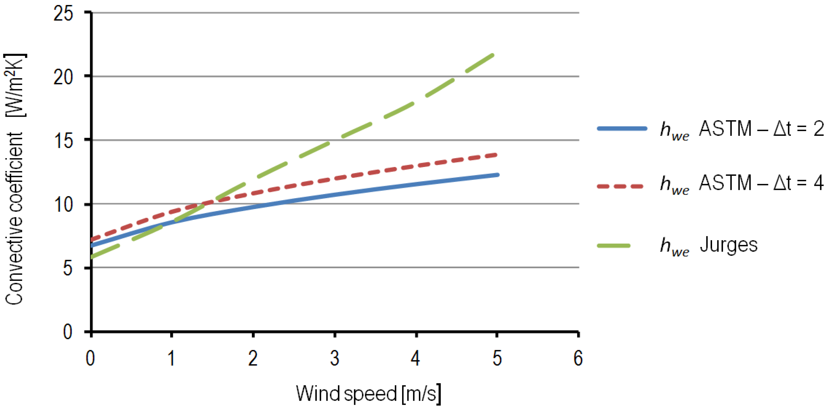
In
Figure 2, it is possible to see the variation of the coefficient
hwe calculated with the Jurges Equation (4) and with Equations (5) and (6) from standard ASTM for two different values of (
ts − tref), considering as a variable the wind speed.
Figure 2.
Variation of hwe coefficient as a function of wind speed.
Figure 2.
Variation of hwe coefficient as a function of wind speed.
It is evident from the figure that the values of the convective coefficient calculated by the two methods are comparable for a wind speed less than 2 m/s. Therefore, in order to simplify the calculation methodology, we will use the Jurges equation that depends only on the wind speed.
It is also observed that when the wind is less than 2 m/s the coefficient value h is less than 10. In this case, the situation becomes more manageable because the temperature difference increases, reducing the margin of error for the calculation of the coefficient.
3.2. Measurement of the Temperature
However, the ΔT that we expect is comparable to the error of the camera. In addition to this we must consider the error introduced by not knowing the exact value of emissivity, the mean radiant temperature, air temperature, distance, humidity, all of which are parameters necessary for the equipment to make the correct conversion of the radiance measured in temperature value. Finally, we should add the error in the measurement of the air temperature with a conventional thermometer.
Thus we measure simultaneously with the camera the temperature of the wall being studied and that of the surface of a portion of unheated building, constructed with the same material (or at least of similar surface density) and having the same surface finish.
The portion will be found to be at a temperature related to the balance between convective and radiative heat transfer. The heated wall will be affected by heat exchange equivalent to the former and additionally by the outgoing heat flow related to thermal losses, for this reason it will have a higher surface temperature.
Therefore, the calculation of the temperature difference takes into account the surface temperature of a wall which is not heated and the surface temperature of the heated wall, with the objective of eliminating or at least minimizing the measurement error due to the use of the thermal camera.
The measurements were made with the same instrument under the same instant and weather conditions, then the errors due to the use of thermal camera are the same. Proceeding in this manner, even if the absolute values of temperature may contain errors which are significant, the final temperature differences will have minimal errors.
4. Infrared Survey
The first important step of a thermographic analysis is the definition of the aim of the survey. The infrared audit procedure is performed in accordance with the available information which needs to be integrated with the necessary building surveys, both qualitative and quantitative. In order to properly evaluate the actual conditions of a building, the professional auditors must acquire information about its architectural, technological and plant characteristics: the situation and conditions of the surroundings (climate included) must also be considered [
6]. The success of a thermographic survey is strongly influenced by several factors such as the minimum environmental requirement, the equipment and the building conditions.
4.1. Minimum Environmental Requirement
The standard EN 13187:1998—Appendix D [
17] describes an example for the best weather conditions for infrared on-site audits in Scandinavian countries. The aim is to guarantee an approximate stable profile of surface temperatures. Those conditions, which are to be evaluated case-to-case in function of the climate peculiarities of the relevant country, are as follows.
- -
For at least the 24 h before the beginning of the infrared audit and during its execution the following relationship must be respected:
where
θin is the interior temperature;
θext the ambient temperature; and
U is the U value (W/m
2 K) of the element being considered. However ∆
θ has to be at least 5 °C.
- -
For at least the 12 h before the beginning of the infrared audit and anyway during its execution, the analysed building surfaces should not be exposed to direct solar radiation.
- -
During the thermographic analysis the exterior and the interior temperature must not vary by more than ±5 °C and ±2 °C, respectively.
If thermographic analysis is to be conducted deviating from the conditions above, it is necessary to explain the motivations for doing so on the thermographic report, which has to be consistent, in its general layout, with the well-defined indications of the EN 13187 standard.
The purpose of our work was to obtain, in an indirect manner, the most reliable range of U-values of opaque walls of building envelopes without knowing the thermo-physical properties of the walls. Even the internal use conditions, i.e., the internal temperature, were unknown. For this reason, the terms of references required by standard EN 13187 have only been partially met.
4.2. Measurement Campaign Survey
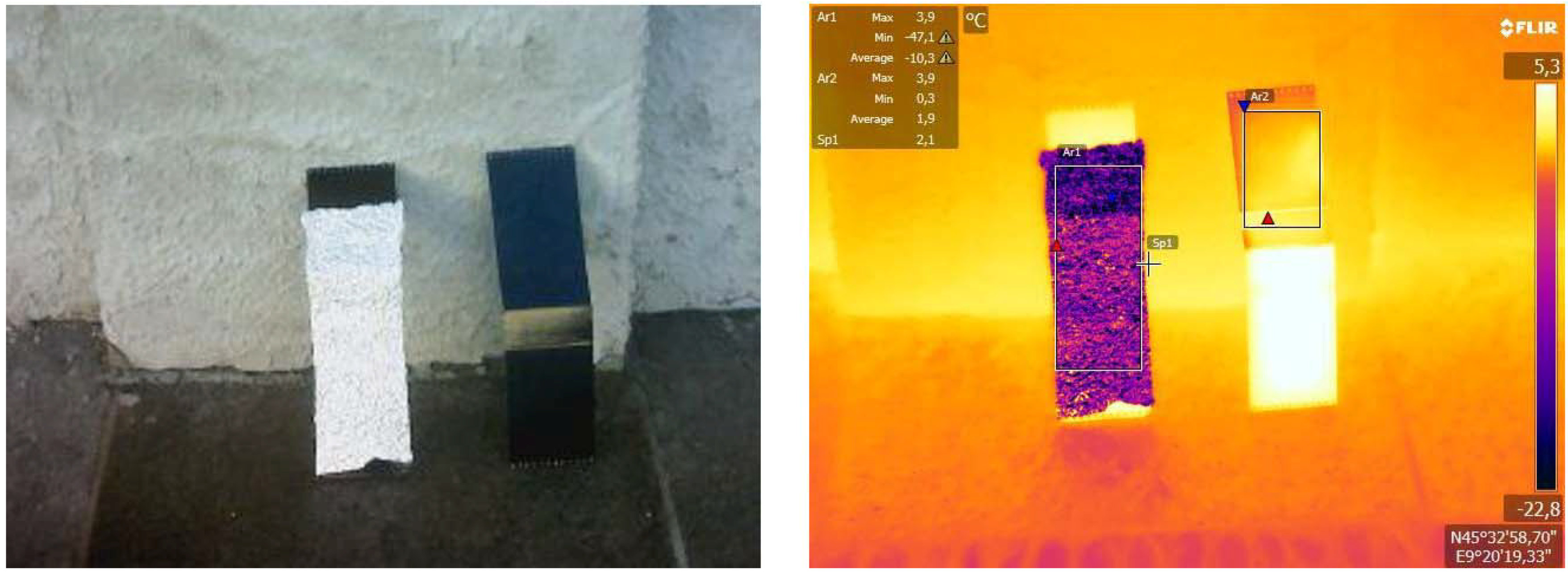
The basic equipment consists of an infrared camera with a spectral sensitivity of 7.8 µm to 14 µm (infrared thermal wavelength range) in order to take infrared thermal images of the building and a cardboard box coated with aluminium for the measurement of the reflected apparent temperature (
Figure 3).
Figure 3.
Visible image and thermogram of the cardboard box coated with aluminium.
Figure 3.
Visible image and thermogram of the cardboard box coated with aluminium.
For the needs of the present study a FLIR T640bx thermal camera was employed.
Table 1 shows the technical characteristics of the infrared camera used during the audit. For this type of application it is important to use a high quality instrument, with high sensor accuracy and the ability to provide images with a high resolution: in this way it is easier to manage homogeneous areas within the thermal image.
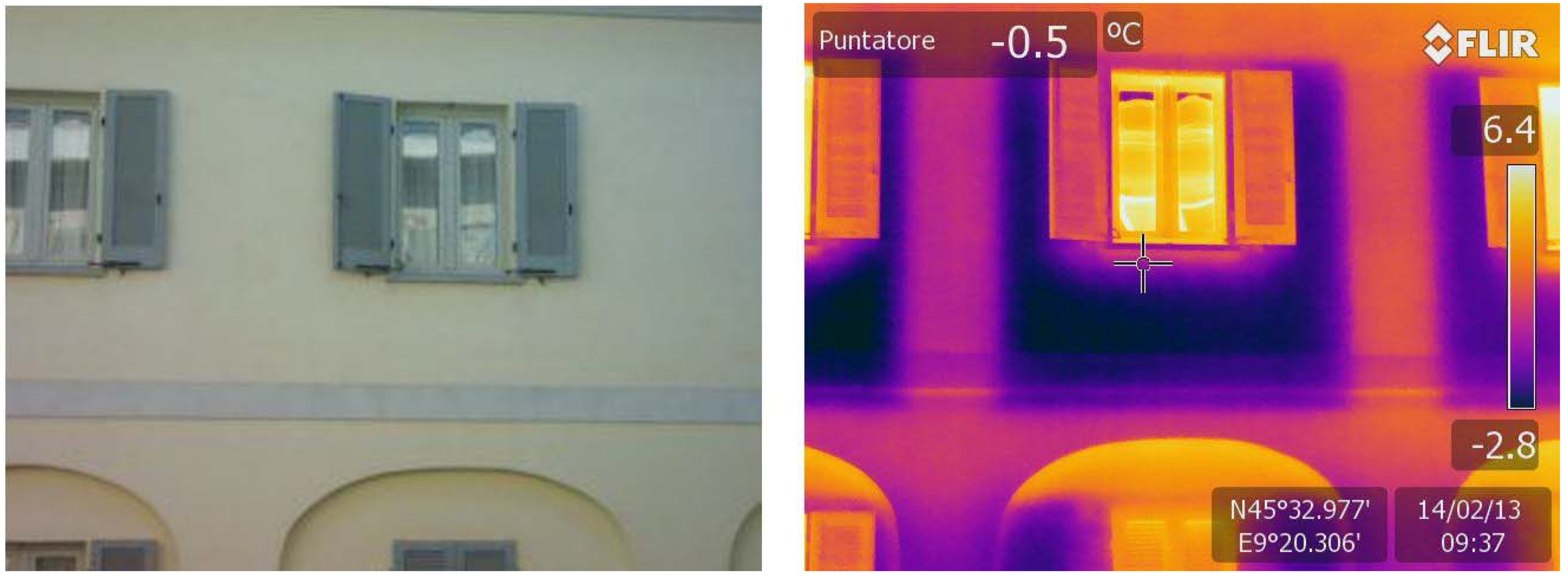
For example,
Figure 4 shows the comparison between the visible image and the infrared image of a part of the wall of the municipal building: one can observe immediately how and where this building has undergone restructuring and where the zones around the windows have been thermally insulated.
Table 1.
Technical specifications of the infrared camera used for the infrared campaign.
Table 1.
Technical specifications of the infrared camera used for the infrared campaign.
| Characteristics | Description | Units |
|---|
| Type | FLIR T640bx | - |
| Spatial resolution | 0.68 (for 25° lens)
0.41 (for 15° lens)
1.23 (for 45° lens) | mrad |
| Thermal sensitivity (at 30 °C) | <35 | mK |
| Spectral range | 7.8–14 | µm |
| Image frequency | 30 | Hz |
| Display | 4.3" superbright touchscreen LCD 800 × 480 pixels | inches |
| Image modes | IR-image with selected color scale
Full color visual
Picture in Picture (Resizable and movable IR- area)
Thermal Fusion (Threshold above, below and interval)
Thumbnail gallery | - |
| Accuracy | ± 2 °C or ± 2% of reading | - |
| Digital zoom | Direct access, 1–8× conditions | - |
| Focus | Continuous, one shot or manual | - |
| Temperature range | −40–+150 | °C |
| Image presentation MSX | IR image with MSX | - |
| Viewfinder | 800 × 400 | pixels |
| Emissivity correction | 0.01–1.0 or selected from materials list | - |
| Measurement correction | Reflected temperature, optics transmission and atmospheric transmission | - |
| Digital camera | 5 incl. lamps | Mpixel |
| Operating temperature range | −15–+50 | °C |
| Humidity, operating and storage, non-condensing | IEC 60068-2-30/24 h
95% relative humidity +25 °C–+40 °C | - |
Figure 4.
Visible image and thermogram of the municipal building.
Figure 4.
Visible image and thermogram of the municipal building.
4.3. Election of the Sample Buildings
The analyzed sample buildings analysed are located in Carugate, a small town near Milan. Carugate is the first Italian city to have approved in 2004, i.e., before the adoption of national and regional energy legislation derived from the transposition of the EPBD, innovative building regulations which imposed restrictive rules to promote energy sustainability of buildings (such as the reduction of U-values of the components of the building envelopes, solar thermal systems mandatory for new buildings, etc.).
The selection of the 14 buildings was made on the basis of the following criteria:
- -
buildings constructed in different historical periods;
- -
buildings erected using local construction techniques and still representative of the specific method of building locally;
- -
buildings with the heating on during the period of investigation;
- -
buildings in which it was possible to retrieve the project technical documentation to establish the values of the thermal transmittance (U-values) of the components of the buildings envelopes.
Once the technical documentation had been acquired, this was analysed with great care and the points on which to perform the infrared audit were identified.
The main features of the buildings are shown in
Table 2, in particular are shown for each building the structural wall characteristics and construction period, the weather conditions under which the survey was carried out and the theoretical value of transmittance.
Table 2.
Data for some variables recorded during the survey.
Table 2.
Data for some variables recorded during the survey.
| Building | Construction year | Wall type (code) | Design U-value (W/m2 K) | External air temperature (°C) |
|---|
| #1 | 1800 | 1 | 1.03 | 4.34 |
| #2 | 1800 | 1 | 1.03 | 1.64 |
| #3 | 1960 | 2 | 1.53 | 4.68 |
| #4 | 1970 | 2 | 1.00 | 4.75 |
| #5 | 1980 | 2 | 1.04 | 3.14 |
| #6 | 1980 | 2 | 1.04 | 4.25 |
| #7 | 1980 | 2 | 1.04 | 3.42 |
| #8 | 1980 | 2 | 1.04 | 6.20 |
| #9 | 1980 | 2/4 | 1.03 | 7.40 |
| #10 | 1997 | 3 | 0.40 | 7.00 |
| #11 | 1997 | 3 | 0.38 | 7.00 |
| #12 | 2003 | 3/4 | 0.39 | 6.10 |
| #13 | 2006 | 4 | 0.28 | 6.20 |
| #14 | 2009 | 4 | 0.20 | 7.90 |
The emissivity of the construction materials is between 0.85 and 0.95 (FLIR documentation), therefore the emissivity has been taken as equal to 0.90 for all surfaces, a mean value of building construction materials.
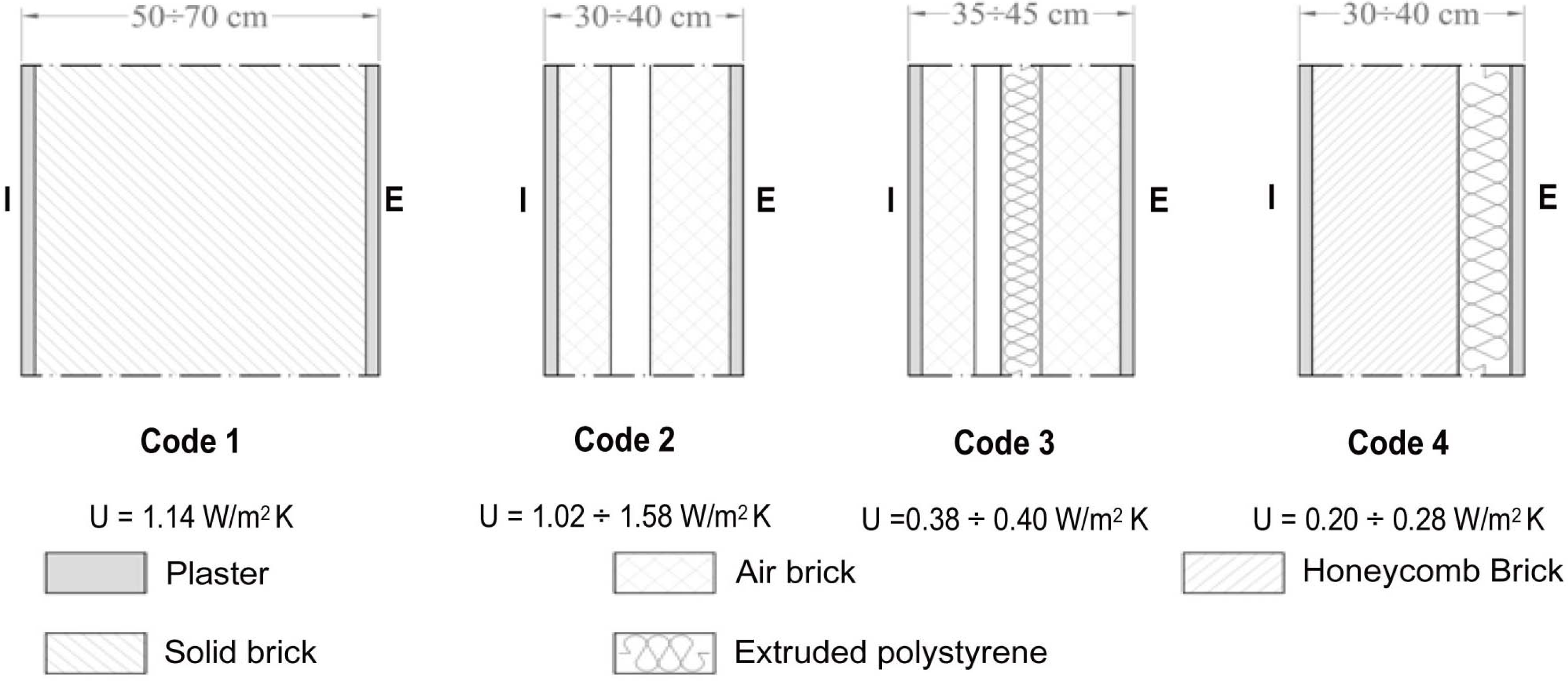
So far as wall type is concerned, we have identified four main types (
Figure 5), which are:
- -
Code 1. the exterior walls of buildings built around 1900 which are very thick and are composed of 50 cm solid brick, with an internal and an external layer of at least 2.0 cm plaster;
- -
Code 2. the most common building solution is the cavity wall, consisting in two brick “skins” separated by a hollow space, with an internal and an external layer of 2.0 cm of plaster;
- -
Code 3. this type has the same stratigraphy as that of the previous type, but additionally within the cavity there is air and a layer of insulating material close to the more external skin;
- -
Code 4. the most recent wall types which are constituted by honeycombed blocks insulated externally with at least 5 cm of extruded polystyrene.
The stratigraphy and the calculation of the transmittance of the wall are derived from the technical report attached to the planning permission.
Figure 5.
Construction details of the external walls.
Figure 5.
Construction details of the external walls.
4.4. Operating Conditions
So far as the internal air temperature of the heated spaces is concerned, the national and regional laws in Italy require it to be 20 °C, for the whole winter period, with a tolerance of 2 °C. Even if the control system is set at 20 °C it is often not able to control the air temperature within the individual rooms and moreover sometimes the users adjust, by means of the local thermostat, the temperature in a different way with respect to the standard conditions, depending on their individual needs.
In a monitoring campaign in residential buildings located in Milan, not far from the location where the test was performed, Dall’O’
et al. [
18,
19] verified the variations of air temperature maintained by the users compared to the standard conditions. For this reason we decided to consider the values of the indoor air to be between the said variations, and then in an indirect way to estimate the U-value: considering a possible range of values of temperature, between 18 °C and 22 °C, two U-values, corresponding to each of these two limiting temperatures, were calculated. In the measurement campaign, the other conditions provided by the EN 13187 standard, and in particular those relating to the climatic conditions to carry out the surveys, were all complied with.
4.5. Site Conditions
For the purposes of our study the conditions at the time of measurement and those recorded in the 24 h preceding the survey were taken into account. Therefore the following conditions were considered as optimal: average low temperature, little wind, overcast sky (so as not to have the radiant temperature too low and solar radiation too high), stable weather conditions. The surveys were organized on the days when climatic conditions as close as possible to those ideal were exactly scheduled. The climate is a very important element in order to obtain accurate and reliable results: for this reason the appropriate conditions to minimise errors arising from any instability have been carefully studied. Our case is a case study, so we carried out a measurement campaign on two days deemed appropriate with respect to a predetermined level. With the results obtained from the measurement in the field, we validated the data against theoretical values taken from the documentation. The weather conditions are highlighted in
Table 3.
Table 3.
Weather conditions.
Table 3.
Weather conditions.
| Condition | Day 1 | Day 2 |
|---|
| Min. | Avg. | Max. | Min. | Avg. | Max. |
|---|
| Air temperature (C°) | −4.10 | −1.12 | 4.20 | −0.30 | 3.54 | 10.3 |
| Wind speed (m/s) | 0.00 | 0.92 | 1.50 | 0.40 | 0.88 | 2.00 |
Generally the direction of the wind influences the total value of the heat transfer convective coefficient. In order to avoid this problem we decided to carry out the measurements on days characterized by the absence of prevailing winds, therefore the direction of the wind varies with continuity.
4.6. Analysis of the Thermal Images
The thermal images were processed through the use of specific software called FLIR TOOLS PLUS version 3.0 in order to obtain the average temperatures of the heat-dissipation surfaces necessary for the purposes of the study. Therefore, on the thermal image areas are identified which are homogeneous, in terms of material and surface finish, and in the software are implemented data which are related to environmental conditions measured at the time of the survey, such as air temperature, target distance (between 10 m and 20 m), relative humidity and reflected temperature.
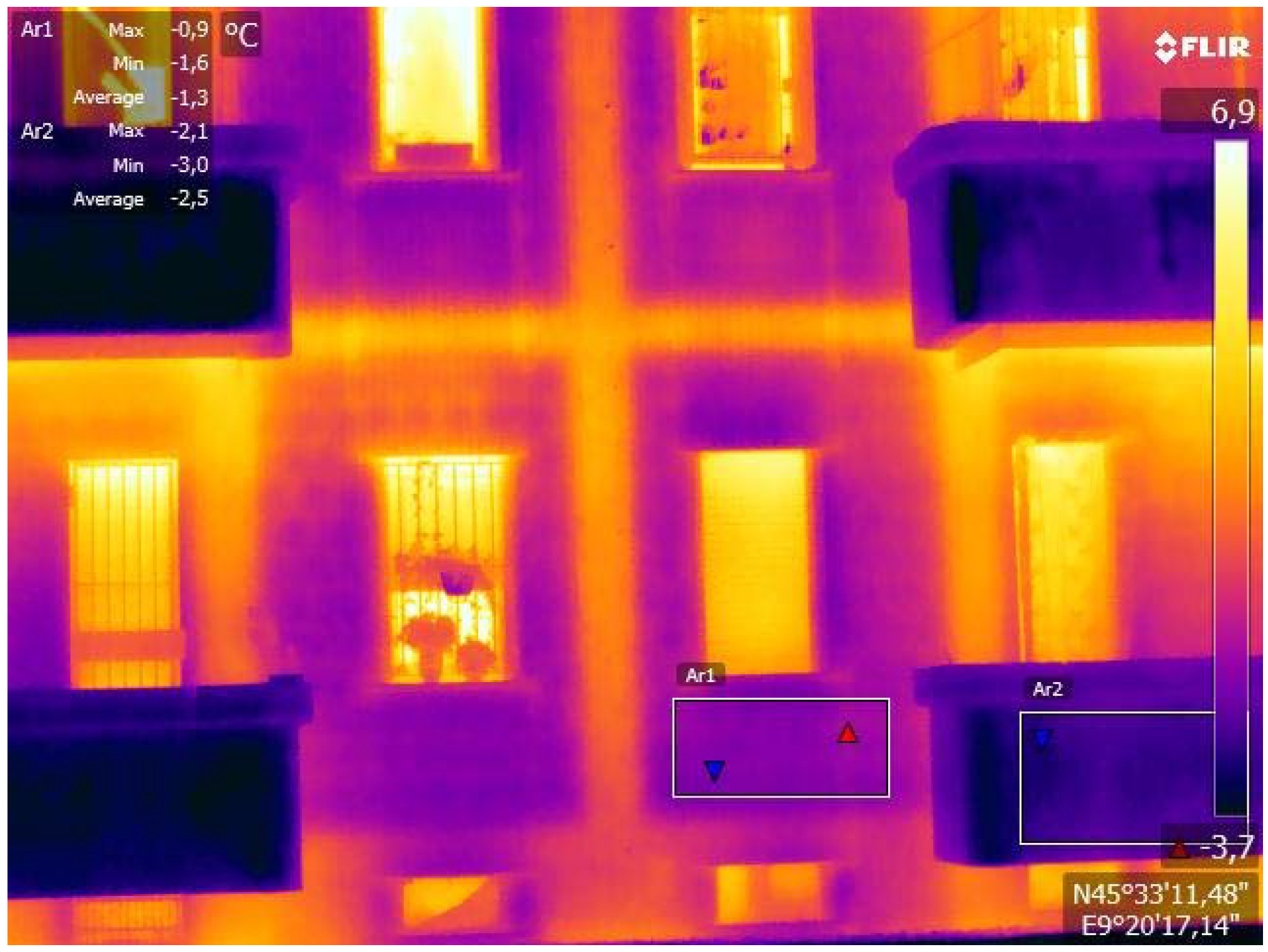
Figure 6 shows a typical example of determination of the areas in order to define the average temperature of heated and non-heated surfaces of the walls.
Figure 6.
Graphic definition of the areas of the wall to evaluate the average temperatures to be considered.
Figure 6.
Graphic definition of the areas of the wall to evaluate the average temperatures to be considered.
5. Results and Discussion
The results of the estimated U-Values for the heating period obtained by applying the IR thermography are given in
Table 4.
Table 4.
Thermal characteristics and percentage absolute deviation between calculated and measured U-value.
Table 4.
Thermal characteristics and percentage absolute deviation between calculated and measured U-value.
| Building | Temp. (°C) | #1 | #2 | #3 | #4 | #5 | #6 | #7 |
|---|
| Reference temperature (C°) | - | 4.6 | −2.8 | 0.5 | −4.2 | 0.6 | −0.1 | −2.1 |
| Average wall temperature (C°) | - | 6.1 | −0.6 | 6.3 | −0.7 | 4.5 | 2.5 | 2.6 |
| Design U value (W/m2 K) | - | 1.03 | 1.03 | 1.53 | 1.00 | 1.04 | 1.04 | 1.04 |
| for v = 1 m/s | Heat flux (W) | - | 10.7 | 15.69 | 41.36 | 24.96 | 27.81 | 18.54 | 33.51 |
| Measured U value (W/m2 K) | 18 | 0.80 | 0.75 | 2.36 | 1.12 | 1.60 | 1.02 | 1.67 |
| 22 | 0.61 | 0.63 | 1.92 | 0.95 | 1.30 | 0.84 | 1.39 |
| Percentage deviation (%) | 18 | −22.8 | −27.0 | 54.8 | 12.3 | 53.4 | −1.7 | 60.0 |
| 22 | −40.5 | −38.8 | 26.0 | −4.8 | 24.7 | −19.5 | 33.5 |
| for v = 0 m/s | Heat flux (W) | - | 8.70 | 12.76 | 33.64 | 20.30 | 22.62 | 15.08 | 27.26 |
| Measured U value (W/m2 K) | 18 | 0.65 | 0.61 | 1.92 | 0.91 | 1.30 | 0.83 | 1.36 |
| 22 | 0.50 | 0.51 | 1.56 | 0.77 | 1.06 | 0.68 | 1.13 |
| Percentage deviation (%) | 18 | −37.2 | −40.7 | 26.0 | −8.6 | 24.8 | −20.0 | 30.2 |
| 22 | −51.6 | −50.2 | 2.5 | −22.6 | 1.5 | −34.5 | 8.6 |
| Building | Temp. (°C) | #8 | #9 | #10 | #11 | #12 | #13 | #14 |
| Reference temperature (C°) | - | 2.8 | 5.7 | 5.0 | 4.2 | 3.0 | 1.9 | 7.0 |
| Average wall temperature (C°) | - | 4.6 | 7.3 | 5.9 | 5.0 | 3.4 | 3.1 | 7.8 |
| Design U value (W/m2 K) | - | 1.04 | 1.03 | 0.40 | 0.38 | 0.39 | 0.28 | 0.20 |
| for v = 1 m/s | Heat flux (W) | - | 12.83 | 11.41 | 6.42 | 5.70 | 2.85 | 8.56 | 5.70 |
| Measured U value (W/m2 K) | 18 | 0.84 | 0.93 | 0.49 | 0.41 | 0.19 | 0.53 | 0.52 |
| 22 | 0.67 | 0.70 | 0.38 | 0.32 | 0.15 | 0.43 | 0.38 |
| Percentage deviation (%) | 18 | −19.0 | −10.3 | 24.9 | 9.7 | −50.7 | 88.1 | 154.0 |
| 22 | −35.8 | −32.3 | −4.5 | −14.9 | −61.1 | 50.6 | 86.3 |
| for v = 0 m/s | Heat flux (W) | - | 10.44 | 9.28 | 5.22 | 4.64 | 2.32 | 6.96 | 4.64 |
| Measured U value (W/m2 K) | 18 | 0.69 | 0.75 | 0.40 | 0.34 | 0.15 | 0.43 | 0.42 |
| 22 | 0.54 | 0.57 | 0.31 | 0.26 | 0.12 | 0.35 | 0.31 |
| Percentage deviation (%) | 18 | −34.1 | −27.0 | 1.6 | −10.8 | −59.9 | 53.0 | 106.6 |
| 22 | −47.8 | −44.9 | −22.3 | −30.8 | −68.4 | 22.5 | 51.5 |
This table presents the percentage absolute deviation between the measured U-values with IR thermography and theoretical expected values. As can be observed, the percentage absolute deviation was found to be at an acceptable level for the solid-mass buildings which possess a high thermal inertia but not for those insulated externally.
For the solid-mass structure buildings encoded with the numbers 1 and 2, it would be appropriate to consider the wind speed equal to one since they are located in isolated and little urbanized areas, while the value of zero for other buildings located in urbanized areas. In the study of a city of Northern Greece [
20], it should be noted that, according to the meteorological data of the Hellenic National Meteorological Service and data analysis, the wind speeds inside the urban canyon in the study area are lower than in the related suburban area. Specifically, the wind speed in the pedestrians’ level (1.8 m) is the 1/3–1/4 of the suburban area. While the wind direction differentiates according the geometry and orientation of the streets.
On the other hand we observe that the percentage absolute deviation for the well insulated wall is very high, being more than 50%. The low thermal inertia of the surface and the limited increase in temperature due to heat flux create a little and unstable temperature difference with respect to reference value. Otherwise when a wall is insulated from the outside the presence of the external thermal insulation composite systems (ETICS) is visible from a first visual investigation and the thickness of the insulating layer can be measured physically without difficulty. The presence of the coat is detectable also thanks to thermal camera by characteristic elements: in the IR image the anchor points of the panels (dowels) are visible; the surface temperature is very close to the temperature of the non heated reference surface.
Therefore, the objective of our study is to acquire knowledge about the actual performance of the wall through a rapid and non-invasive investigation for the buildings constructed more than thirty years ago, for which it is very difficult to find the design documents in which the stratigraphy and the actual transmittances of the envelope are described.
A meaningful advantage of the measurement of the U-value by means of the infrared thermovision technique [
13] is that it is not a point measurement but considers all the surface of the element whose global thermographic image is taken; in this way the areas with anomalous thermal behaviour (local thermal bridges, areas with high moisture,
etc.) can be rejected. This type of issue cannot be resolved if the measurements are performed with the heat flowmeter. Therefore one must be careful to use it in order to obtain a representative average of the heat flow: the sensors must be mounted in such a way so as to ensure a result which is representative of the whole element, avoiding thermal bridges, particular construction joints,
etc.The predominant type of the external wall in Italy is the cavity wall, whose characteristic is by strong temperature variability owing to the convective air movements inside the cavity. In this case the method of thermography provides the most effective detection. Observing
Table 5, it is apparent that with only one measurement an IR image is obtained from which can be calculated precisely the variations in surface temperature and, furthermore, the average value of the homogeneous portion of external wall. The heat flowmeter method would have required for this type of monitoring the use of different probes and over a long period.
That the infrared thermovision technique (ITT) is more accurate than the heat flowmeter method is also demonstrated by the study carried out by Albatici and Tonelli [
13], one of the rare studies that have had the objective of determining the thermal transmittance of building elements by means of thermal flowmeter method (HFM). In particular, they have measured on site the envelope thermal transmittance value for a single family house using two methods, based on the ISO 9869: the average method and the dynamic method. The main difference between the methods is that with the former, the greater is the number of data recorded, the higher is the possibility of obtaining a correct final result. With the second method, the test duration can be shorter but higher indoor-outdoor temperature variation is necessary.
Table 5.
Heat flow in a cavity wall.
![Energies 06 03859 i001]()
Table 5.
Heat flow in a cavity wall.![Energies 06 03859 i001]()
| Spotmeters | Flux (W) | Trasmittance* (W/m2 K) |
|---|
| Sp_1 | 37.79 | 1.88 |
| Sp_2 | 18.54 | 0.92 |
| Sp_3 | 11.41 | 0.57 |
They carried out the test in the month of January, the coldest period of the year in Italy and data were acquired every 15 min, but only some sub-periods suitable for the measurement were considered. In this particular case the average method is not the most suitable: only the results obtained with the dynamic one should be considered. Rejecting the value of 0.74 which is too far away from the others, the average U-value of the external wall measured with the HFM method is 0.48 W/m2 K. It is a value 65% higher than the theoretical value of 0.29 W/m2 K.
Looking at the individual results shown in
Table 6, it can be observed that the maximum percentage deviation is referred to the case of average method with a deviation of 175.8%, whilst the more reliable result is obtained with dynamic method with a 37.9% deviation.
Table 6.
U-value of the external wall using the HFM method.
Table 6.
U-value of the external wall using the HFM method.
| Period | U-value (W/m2 K) average method | Percentage deviation (%) | U-value (W/m2 K) dynamic method | Percentage deviation (%) |
|---|
| 12–12 to 17–12 | 0.68 | 134.48% | 0.49 | 68.97% |
| 26–12 to 3–1 | 0.68 | 134.48% | 0.54 | 86.21% |
| 1–1 to 7–1 | 0.72 | 148.28% | 0.74 | 155.17% |
| 4–1 to 7–1 | 0.80 | 175.86% | 0.40 | 37.93% |
| 23–1 to 27–1 | 0.71 | 144.83% | 0.48 | 65.52% |
The order of magnitude of possible error proves to be much higher than the values of our study. Hence the HFM is much more expensive in terms of execution time and data processing, as well as being far less precise when compared to the ITT.
The survey method proposed has some critical aspects mainly owing to the variability and the large number of parameters involved in the analysis and investigation. The following issues have been identified:
The temperature differences are small values and difficult to monitor with accuracy;
The infrared camera has large absolute errors compared to the values of temperature to be measured;
It is often impossible to know the compensation parameters (emissivity, reflected temperature, etc.) necessary to obtain the correct value of temperature;
The convective coefficient to be used in the formula has a significant influence on the result and must therefore be a real and not a standard value;
The climatic parameters may vary considerably during the execution of the measurement.
To resolve each of the problems highlighted above we have developed the following solutions:
- -
A day is chosen which is deemed appropriate for the purposes of our investigation, looking at the weather forecast of the previous 24 h (cold, little wind, cloud cover). The conditions should possibly persist: in any case the conditions set out in the standard (rain, sun, etc.) must be avoided (this solves point 1);
- -
The method is limited to high thermal mass walls and it is not valid for externally insulated walls (this solves points 1 and 5);
- -
We use as reference temperature the external temperature measured with the same thermal camera for a non-dissipating portion of the same masonry (solution for points 2 and 3);
- -
In any case data to perform the compensation of the measurement were detected, excluding the determination of emissivity, in order to minimize the error in the determination of the temperature difference;
- -
The convective coefficient h is estimated considering the average wind speed of the previous hours, since it is not important to have the instantaneous value, especially for walls with high thermal inertia. Thus, the h value was calculated in a more sophisticated way than that indicated in the literature which refers almost exclusively to the values given by standard (this solves point 4).
6. Conclusions
The possibility of using IR inspections to obtain not only qualitative but also quantitative information, on the basis of which one can for example make an indirect evaluation of the U-value of the walls in existing buildings, has been the subject of many studies and research, and indeed many more studies and research will be done in the future. The complexity of the process of interpreting infrared images is largely due to the complexity of the physical phenomenon of heat transfer in real buildings, but especially to the many variables involved which are often dependent on meteorological phenomena.
In recent years, however, the technology of infrared cameras has advanced and thermal maps generated by the latest models offer a lot of information in terms of image definition (significant increase in the number of pixels). The information is also more accurate because of the better quality of the IR sensors. The software for image processing has advanced the most, in terms of graphics management of the pictures: from a single shooting is now possible to make many more evaluations, changing the parameters, locate homogeneous areas and make very precise calculation of the average values of temperatures.
There are also fields of application in which it is not necessary to obtain accurate information: one of these is the infrared screening of existing buildings for the purpose of preliminary diagnostics. This type of approach can be very useful in those cases where there is the need to perform IR mappings of a significant number of buildings, or building stocks, with limited time and limited budget. The research presented and discussed in this paper should be seen precisely in this field of application.
The results presented show that it is possible to use sufficiently reliable infrared diagnostics to make evaluations on energy performance (U-values) of existing buildings, as long as some appropriate precautions are taken.
The proposed methodology does not allow the determination of a single value of transmittance but rather a range within which the value is likely to lie, through an investigation method which is rapid and non-invasive. The comparison between the range of transmittance values obtained and the real ones derived from documentation provided, shows that this method, in the case of buildings with externally insulated walls is not very reliable because the errors are high (see
Table 4, cases #13 and #14).
On the other hand, the survey found that this type of evaluation is reliable for solid-mass walls, for which the error percentage is lower if compared to thermal flowmeter method (see
Table 4, cases from #1 to #12).
Therefore, the application of the methodology to the single building for different portions of the envelope, as well as the validation of the results through the application of statistical methods will be the subject of subsequent, future studies.


