Analysis of Future Vehicle Energy Demand in China Based on a Gompertz Function Method and Computable General Equilibrium Model


Abstract
:1. Introduction


2. Methodology and Data

2.1. Gompertz Function
2.2. Computable General Equilibrium (CGE) Model

| No. | Sector | No. | Sector |
|---|---|---|---|
| 1 | Agriculture, forestry, animal husbandry and fishery | 22 | Scrap waste |
| 2 | Coal mining and washing | 23 | Electricity, heat production and supply industry |
| 3 | Oil and gas exploration industry | 24 | Gas Production and Supply |
| 4 | Metal mining industry | 25 | Water production and supply industry |
| 5 | And other non-metallic mineral mining industry | 26 | Construction |
| 6 | Food manufacturing and tobacco processing industry | 27 | Transportation and Warehousing |
| 7 | Textile industry | 28 | Postal Services |
| 8 | Textile, leather and feather products industry | 29 | Information transmission, computer services and software industry |
| 9 | Wood processing and furniture manufacturing | 30 | Wholesale and retail trade |
| 10 | Paper printing and Educational and Sports Goods | 31 | Accommodation and Catering Services |
| 11 | Petroleum processing, coking and nuclear fuel processing industry | 32 | Financial Industry |
| 12 | Chemical Industry | 33 | Real Estate |
| 13 | Non-metallic mineral products industry | 34 | Leasing and Business Services |
| 14 | Metal smelting and rolling processing industry | 35 | Research and Development Industry |
| 15 | Fabricated Metal Products | 36 | Integrated Technical Services |
| 16 | General, special equipment manufacturing industry | 37 | Water conservancy, environment and public facilities management industry |
| 17 | Transportation Equipment Manufacturing | 38 | Resident Services and Other Services |
| 18 | Electrical machinery and equipment manufacturing | 39 | Education |
| 19 | Communications equipment, computers and other electronic equipment manufacturing | 40 | Health, social security and social welfare |
| 20 | Measuring Instruments and Office Machinery | 41 | Culture, Sports and Entertainment |
| 21 | Handicrafts and other manufacturing | 42 | Public administration and social organizations |
2.2.1. Production
2.2.2. Income Distribution, Taxation and Transfer
2.2.3. Domestic Demand
2.2.4. Foreign Trade
2.2.5. Model Closure and Market Clearing
2.2.6. Dynamic Structure
2.3. Energy Consumption
2.4. Data
3. Results and Discussion
3.1. Results
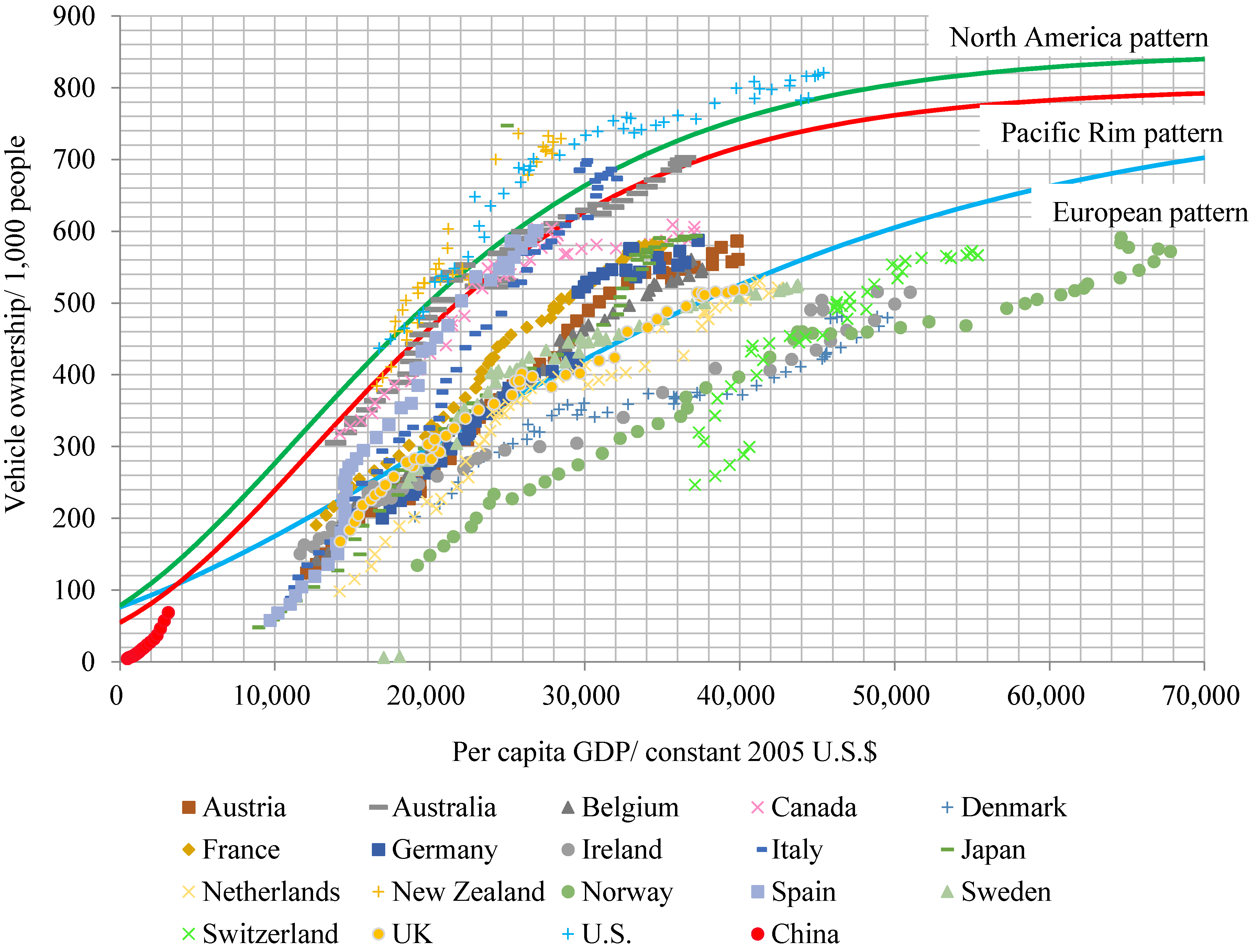
3.1.1. Curvature Parameters in the Gompertz Function
| Dependent Variable: | ||||||
|---|---|---|---|---|---|---|
| Variable | North America Pattern | Pacific Rim Pattern | European Pattern | |||
| RE | FE | RE | FE | RE | FE | |
| −0.887 *** | −0.755 *** | −0.797 *** | −0.800 *** | −0.436 *** | −0.443 *** | |
| (−17.60) | (−24.29) | (−28.82) | (−29.29) | (−35.78) | (−36.56) | |
| 1.249 *** | 0.870 *** | 0.960 *** | 0.988 *** | 0.825 *** | 0.844 *** | |
| (8.30) | (9.41) | (5.10) | (14.82) | (10.66) | (23.12) | |
| N | 96 | 96 | 139 | 139 | 630 | 630 |
| Coefficients | Hausman test | ||||||
|---|---|---|---|---|---|---|---|
| (b) Fixed | (B) Random | (b−B) Difference | Standard Error | chi2 (1) | Prob > chi2 | ||
| North America pattern | |||||||
| −0.0000755 | −0.0000887 | 0.0000132 | 1.67 × 10⁻⁶ | 62.15 | 0.0000 | ||
| Pacific Rim pattern | |||||||
| −0.0000800 | −0.0000797 | −3.05 × 10⁻⁷ | 1.41 × 10⁻⁷ | 4.68 | 0.0304 | ||
| European pattern | |||||||
| −0.0000443 | −0.0000436 | −6.37 × 10⁻⁷ | 1.47 × 10⁻⁷ | 18.75 | 0.0000 | ||
| Parameters | North America Pattern | Pacific Rim Pattern | European Pattern |
|---|---|---|---|
| α | −2.387 | −2.686 | −2.326 |
| β | −0.755 × 10⁻⁴ | −0.800 × 10⁻⁴ | −0.443 × 10⁻⁴ |
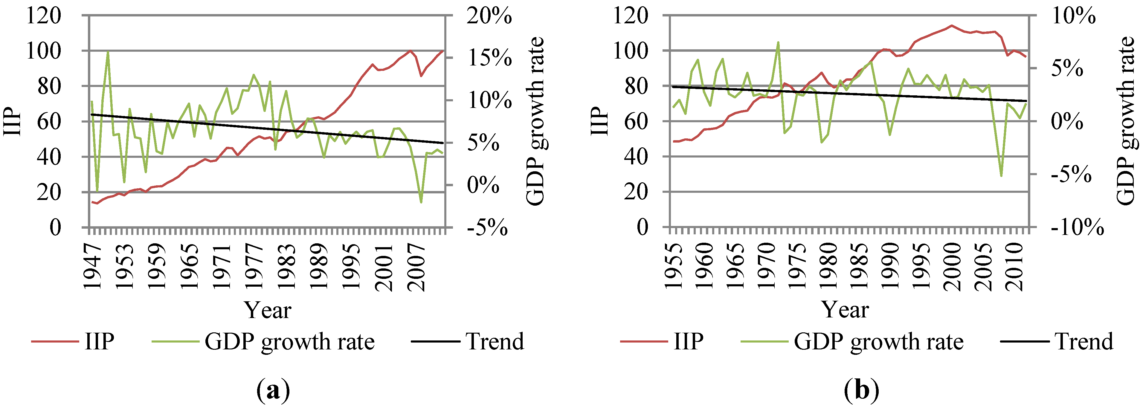
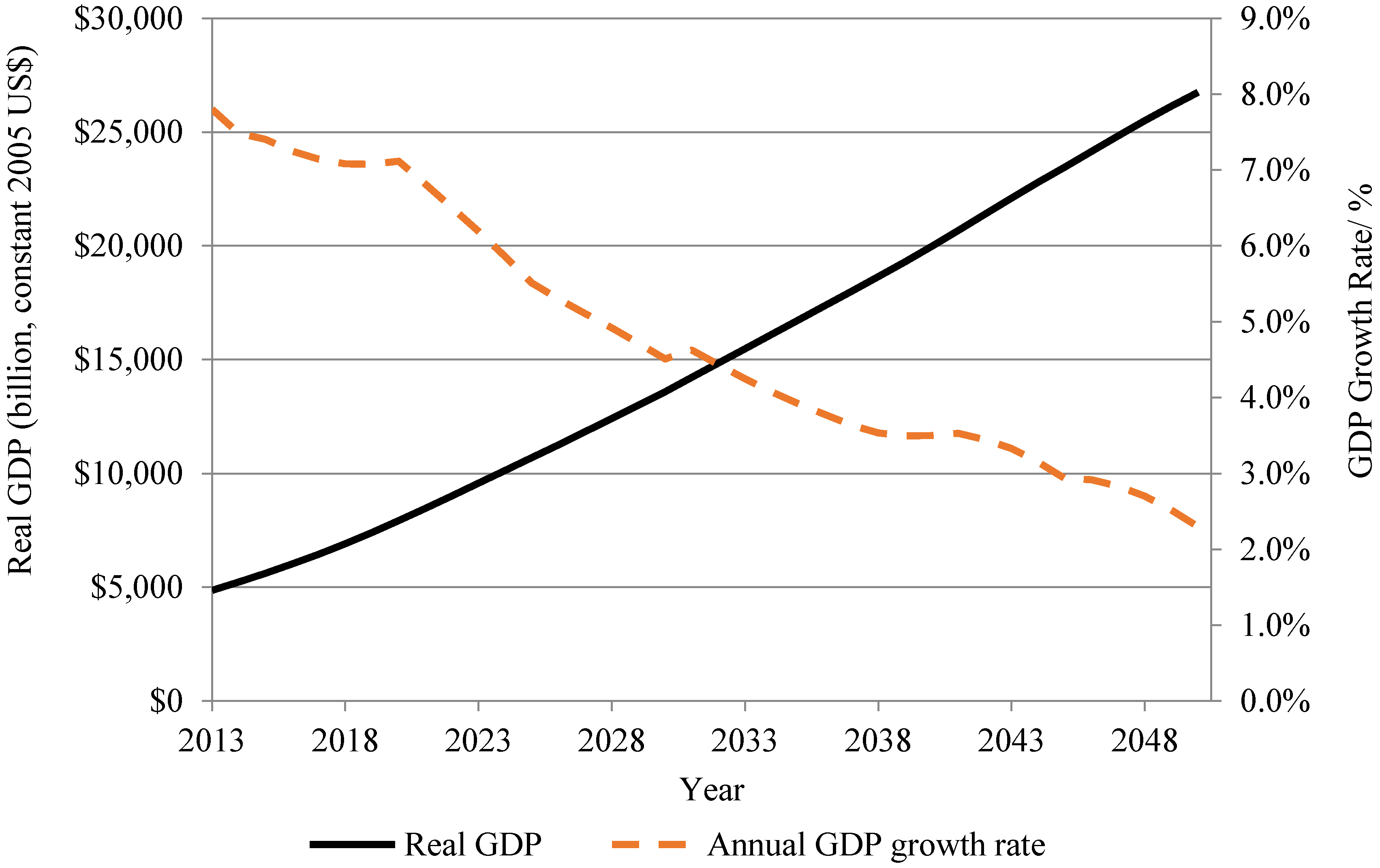
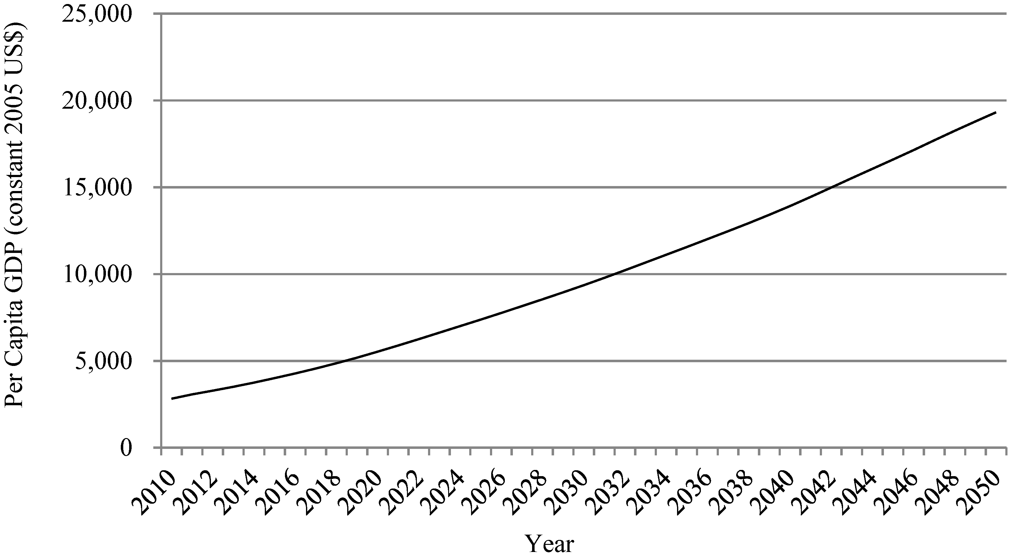
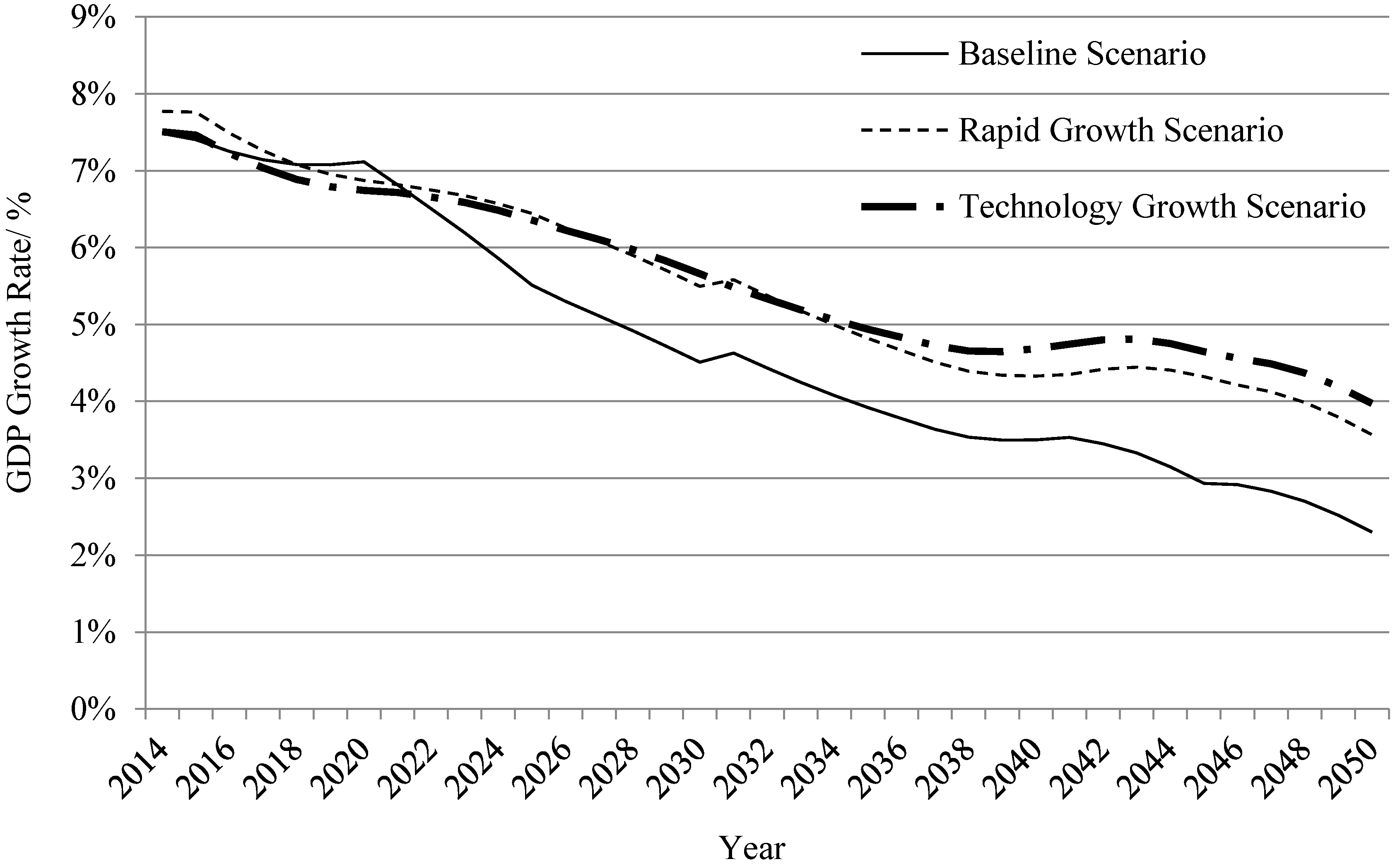
3.1.2. GDP Growth in China


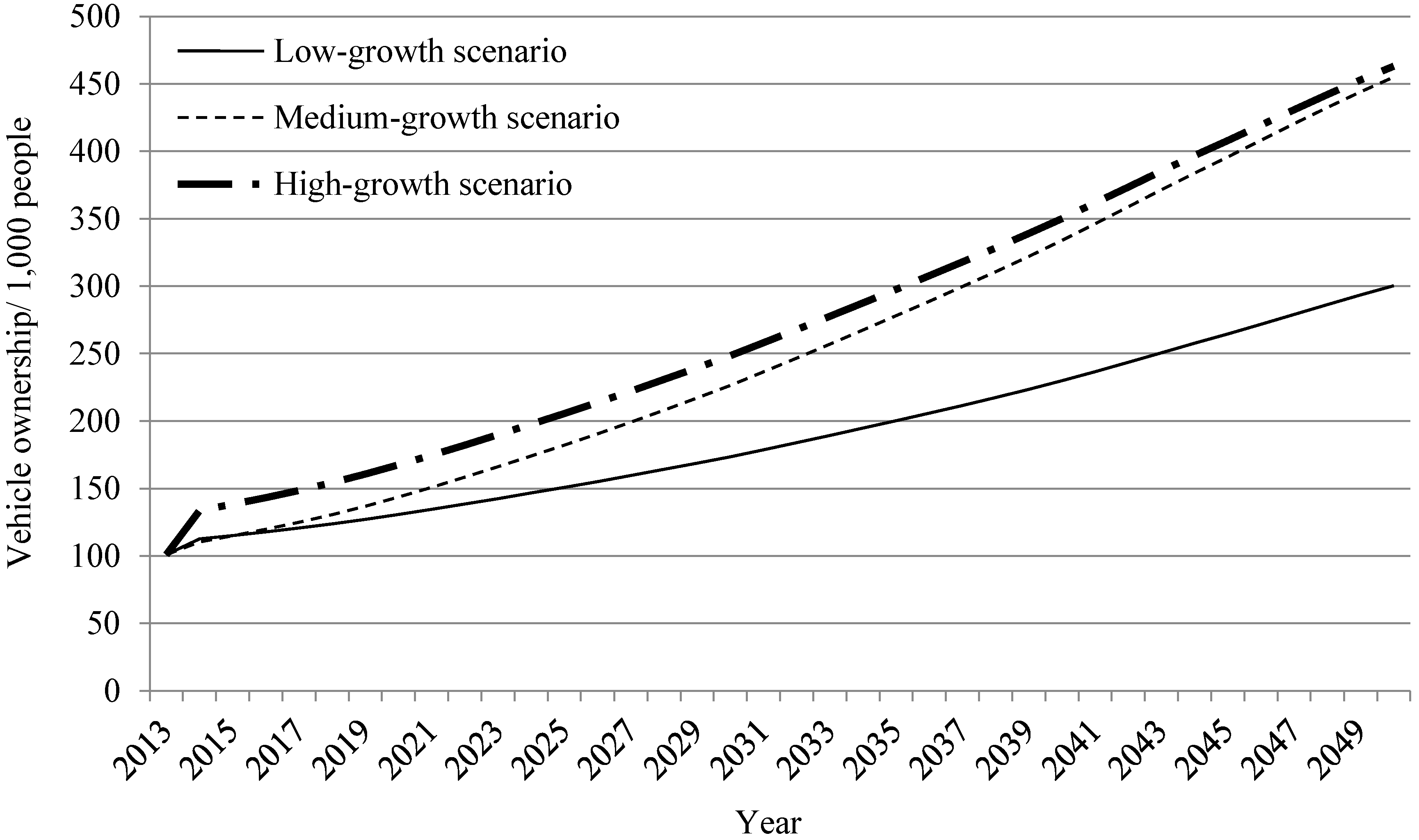
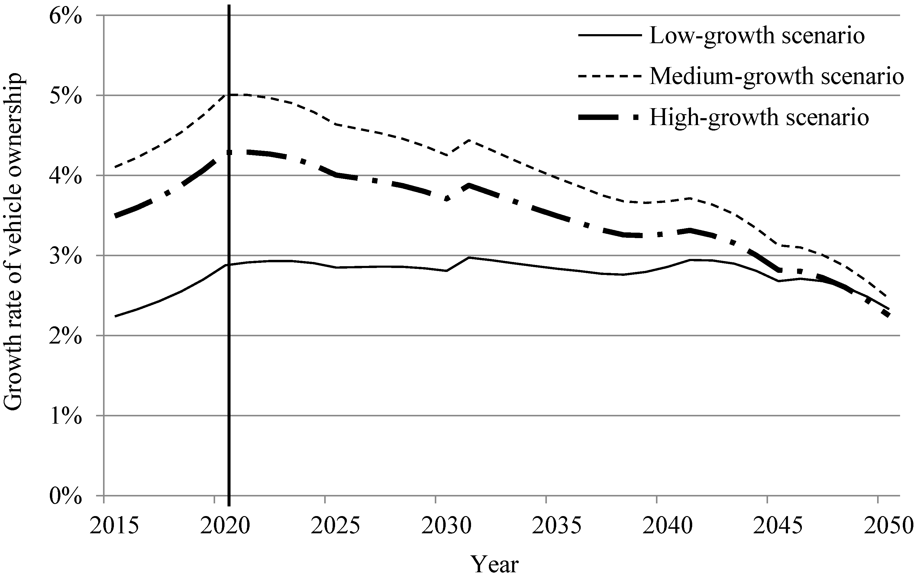
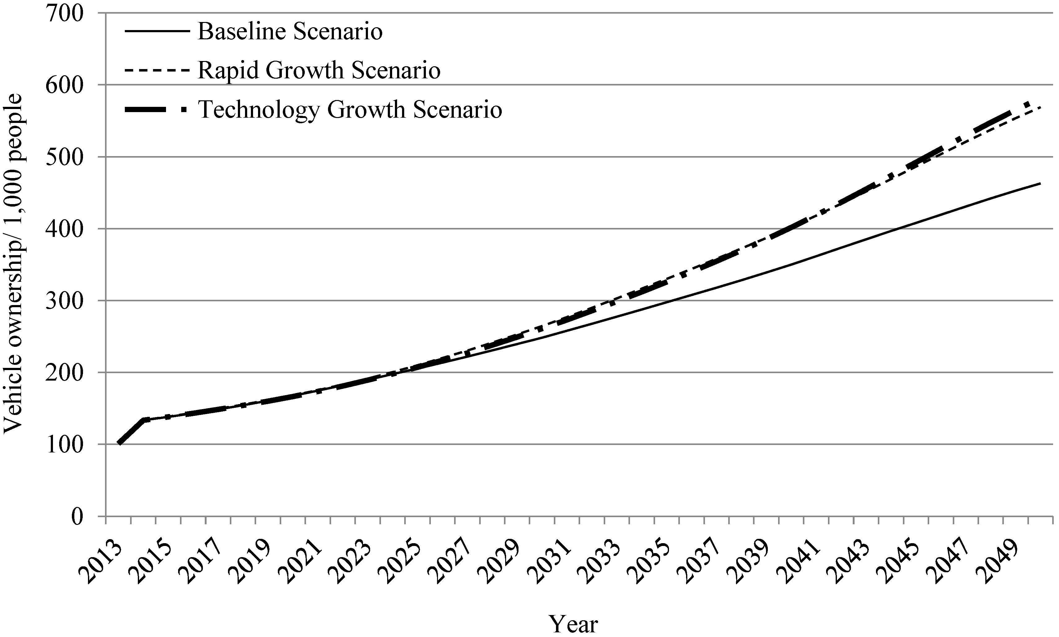
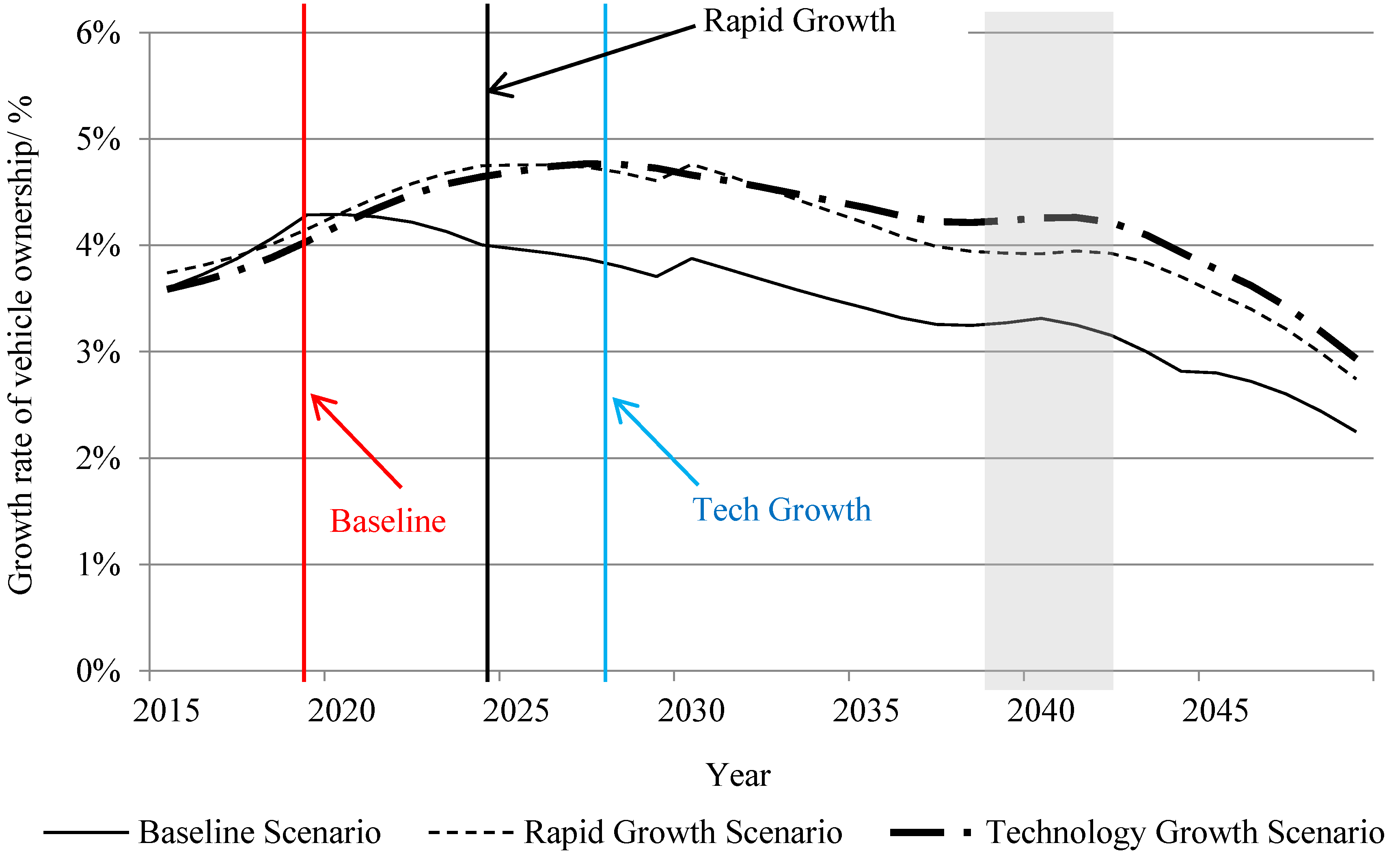
3.1.3. Projection of Chinese Vehicle Ownership


3.1.4. The Energy Demand of Road Vehicles
| Year | Low-Growth Scenario | Medium-Growth Scenario | High-Growth Scenario | |||||||||
|---|---|---|---|---|---|---|---|---|---|---|---|---|
| Car | Bus | Truck | Total | Car | Bus | Truck | Total | Car | Bus | Truck | Total | |
| 2013 | 101.6 | 22.6 | 93.1 | 217.4 | 101.6 | 22.6 | 93.1 | 217.4 | 101.6 | 22.6 | 93.1 | 217.4 |
| 2015 | 115.0 | 20.5 | 89.4 | 225.0 | 114.8 | 20.5 | 89.2 | 224.5 | 138.2 | 24.7 | 107.4 | 270.3 |
| 2020 | 130.8 | 19.2 | 93.2 | 243.2 | 143.7 | 21.1 | 102.5 | 267.3 | 167.6 | 24.6 | 119.5 | 311.7 |
| 2025 | 132.1 | 19.5 | 107.7 | 259.3 | 159.5 | 23.6 | 130.1 | 313.2 | 180.0 | 26.6 | 146.9 | 353.5 |
| 2030 | 137.5 | 19.8 | 118.3 | 275.6 | 179.4 | 25.8 | 154.3 | 359.5 | 196.8 | 28.3 | 169.4 | 394.5 |
| 2035 | 147.1 | 21.6 | 138.0 | 306.7 | 204.2 | 29.9 | 191.7 | 425.8 | 218.6 | 32.1 | 205.2 | 455.8 |
| 2040 | 155.1 | 23.0 | 151.0 | 329.0 | 225.2 | 33.4 | 219.3 | 477.9 | 236.2 | 35.0 | 230.0 | 501.2 |
| 2045 | 166.7 | 25.4 | 165.6 | 357.7 | 249.4 | 38.0 | 247.8 | 535.1 | 257.0 | 39.1 | 255.4 | 551.6 |
| 2050 | 176.8 | 27.4 | 175.5 | 379.7 | 267.9 | 41.5 | 266.0 | 575.4 | 272.7 | 42.2 | 270.7 | 585.5 |
3.2. Discussion on Key Factors

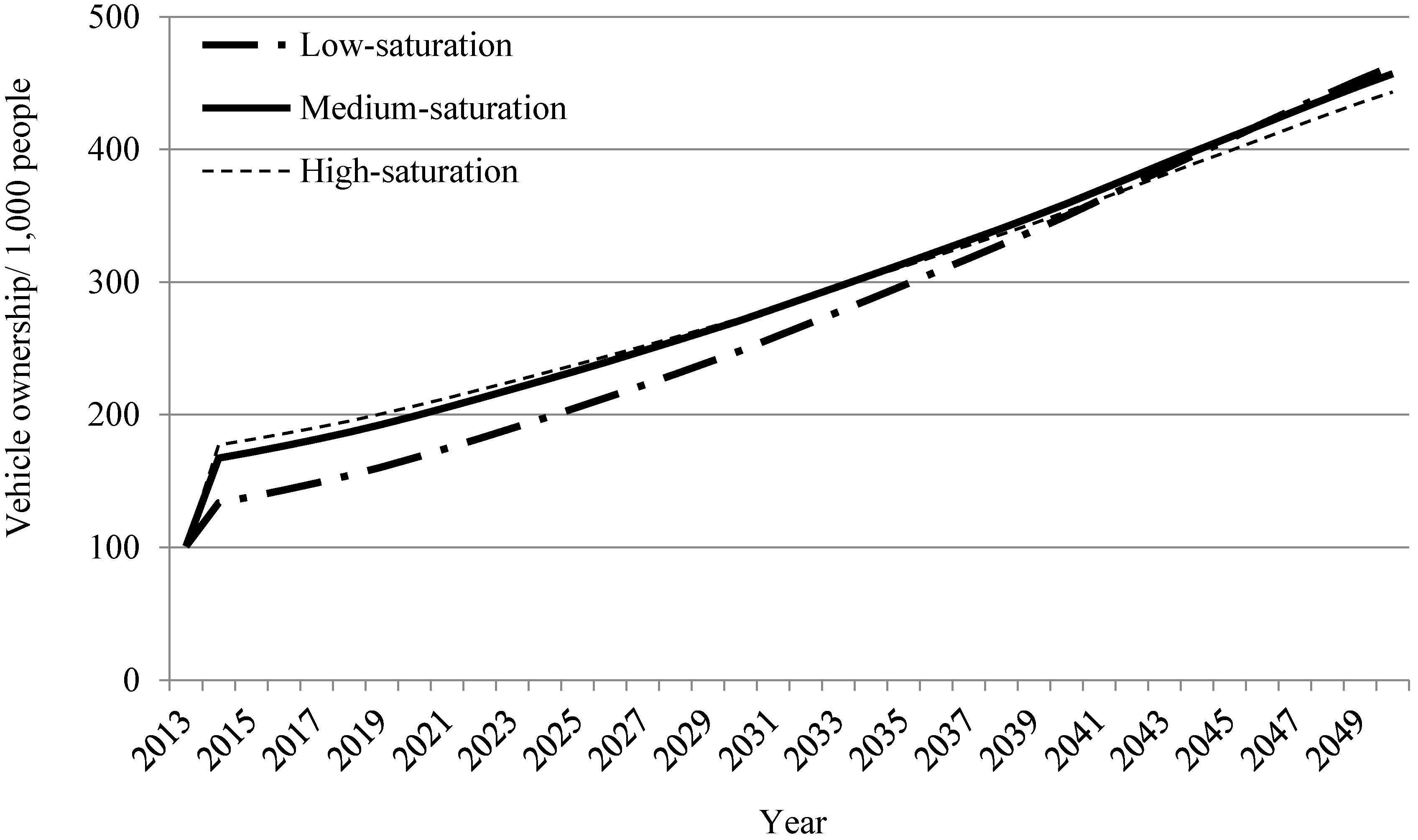
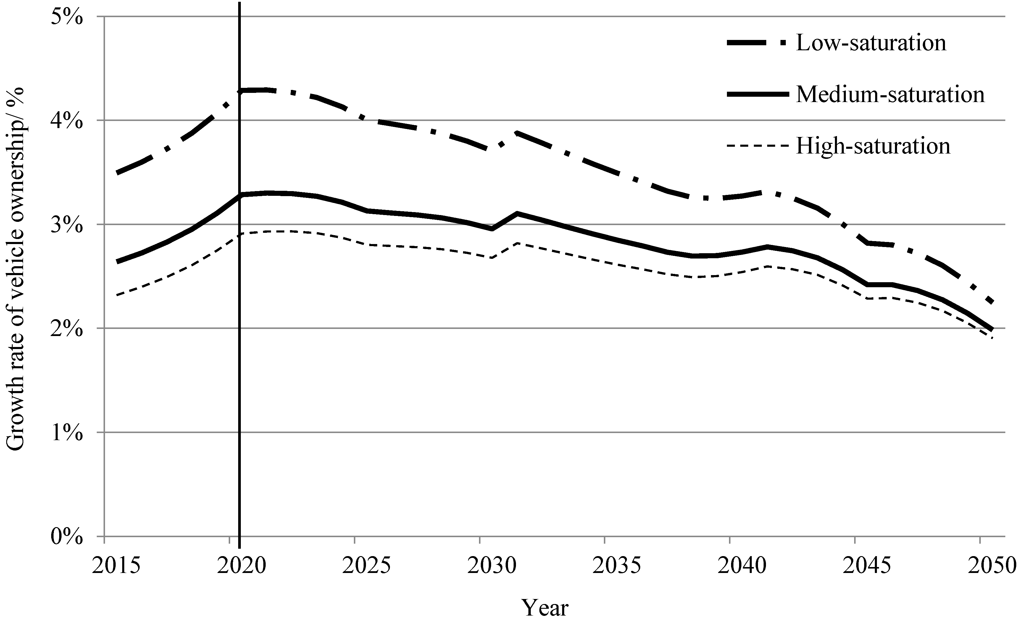
3.2.1. Sensitivity Analysis of Vehicle Saturation Levels
| Country | Low-Saturation | Medium-Saturation | High-Saturation |
|---|---|---|---|
| Dargay et al. [20] | Wu et al. [15] | Dargay and Gately [19] | |
| Canada | 845 | 860 | 910 |
| United States | 852 | 875 | 890 |
| α | −2.387 | −2.010 | −1.896 |
| β | −0.755 × 10⁻⁴ | −0.654 × 10⁻⁴ | −0.597 × 10⁻⁴ |


3.2.2. Sensitivity Analysis of GDP Growth


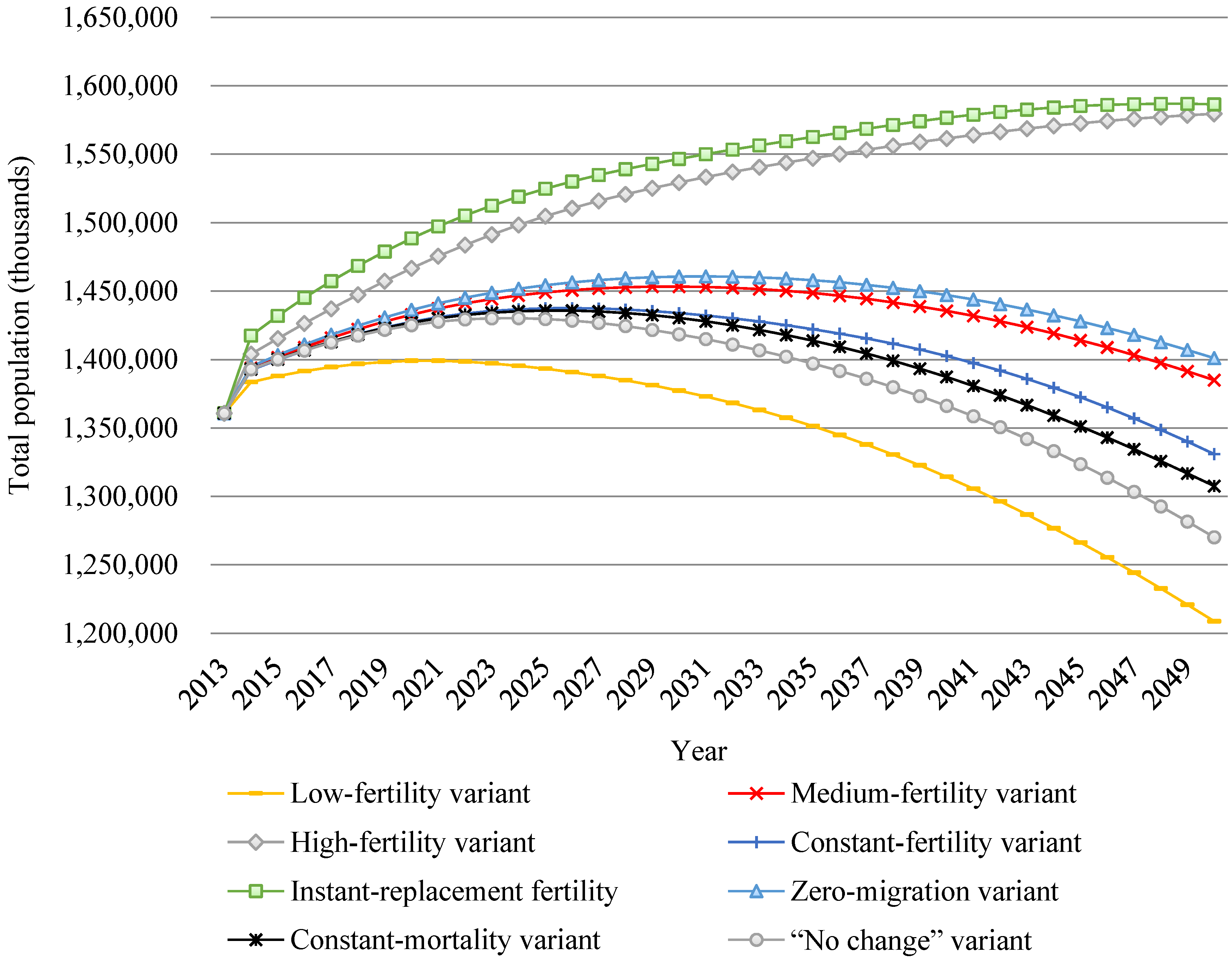
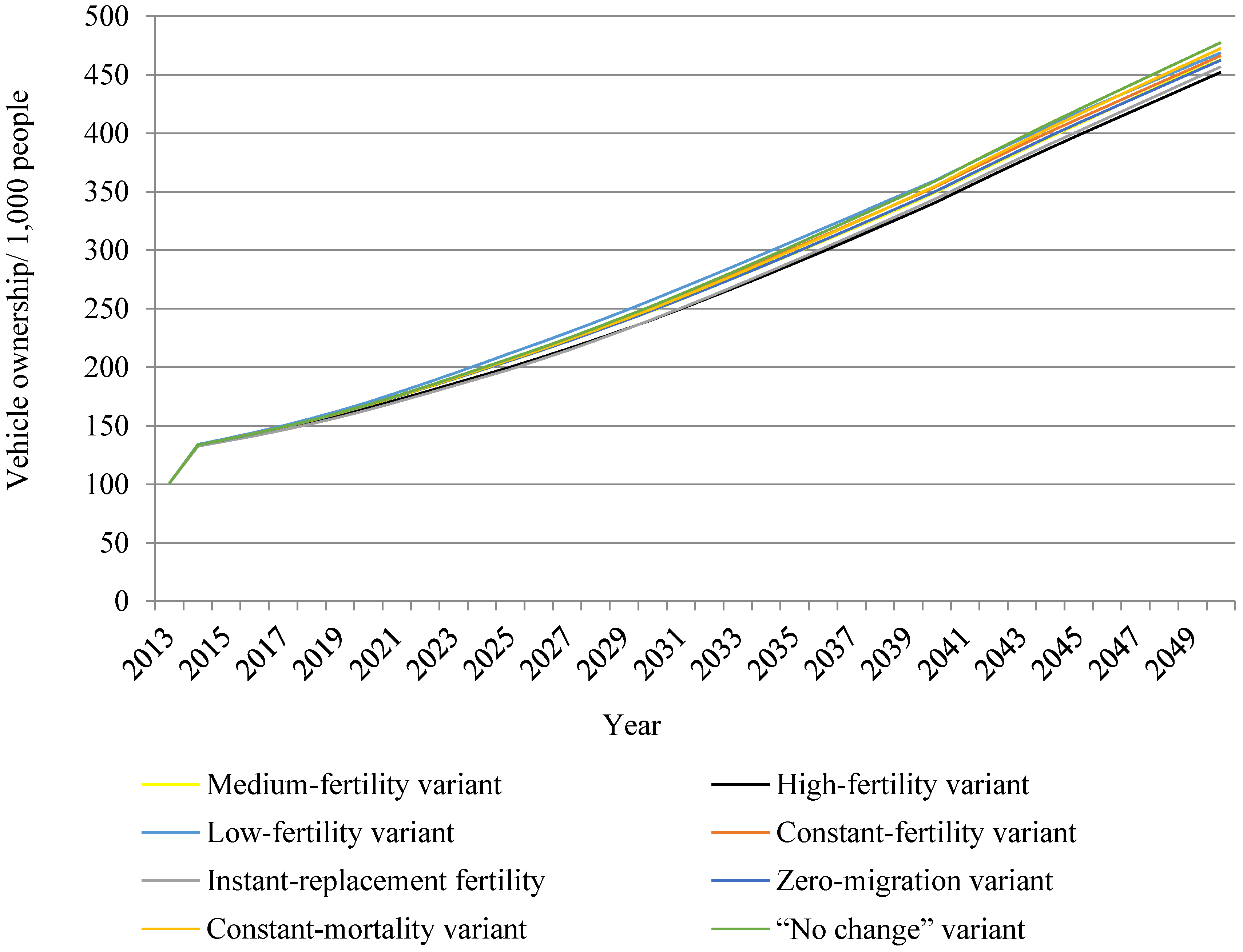
3.2.3. Sensitivity Analysis of Population Growth


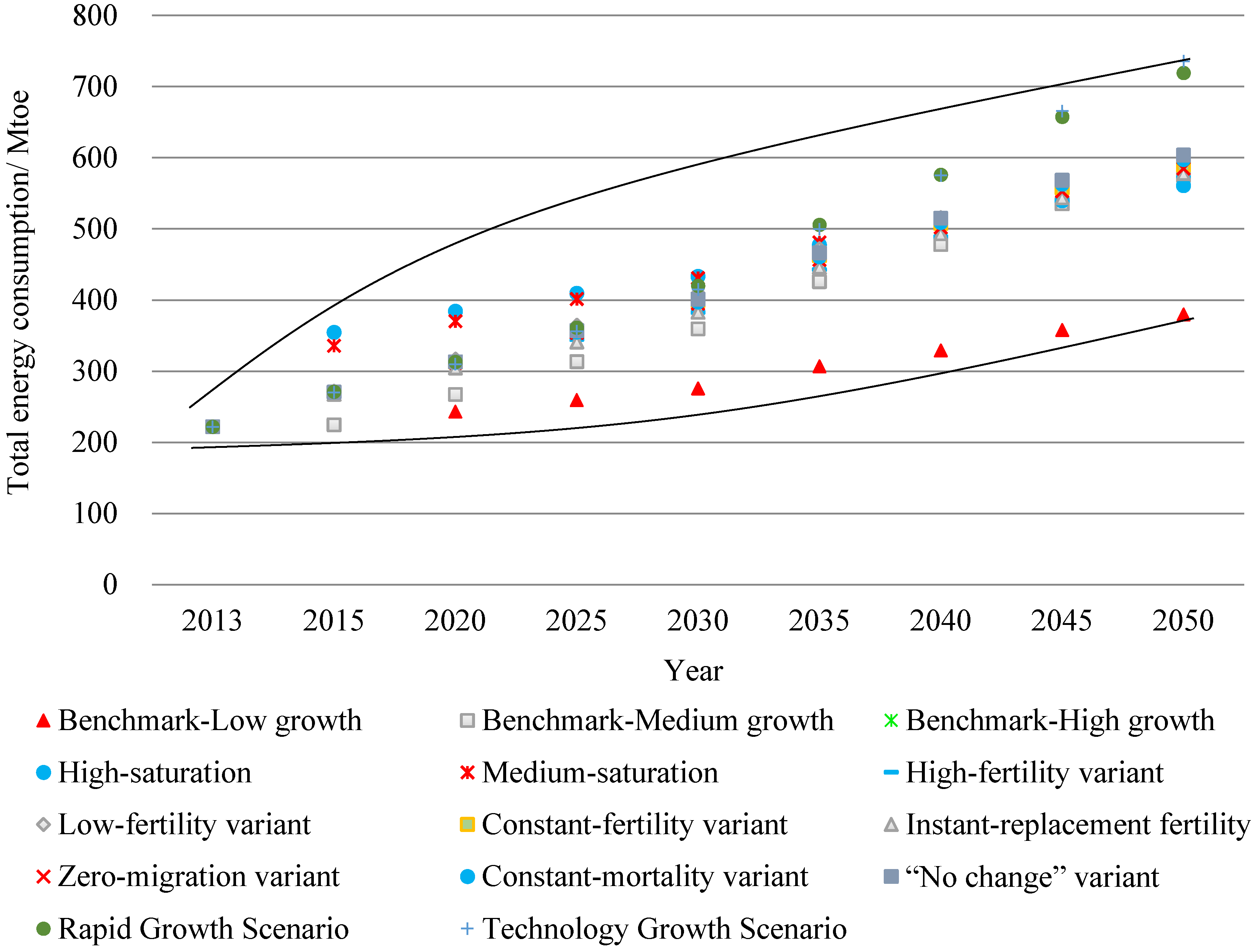
3.2.4. Energy Consumption Projections under Different Scenarios

4. Concluding Remarks
Acknowledgments
Author Contributions
Conflicts of Interest
References
- Waraich, R.A.; Galus, M.D.; Dobler, C.; Balmer, M.; Andersson, G.; Axhausen, K.W. Plug-in hybrid electric vehicles and smart grids: Investigations based on a microsimulation. Transp. Res. Part C Emerg. Technol. 2013, 28, 74–86. [Google Scholar] [CrossRef]
- Yuan, J.H.; Hou, Y.; Xu, M. China’s 2020 carbon intensity target: Consistency, implementations, and policy implications. Renew. Sustain. Energy Rev. 2012, 16, 4970–4981. [Google Scholar] [CrossRef]
- Ou, X.; Yan, X.; Zhang, X.; Zhang, X. Life-Cycle Energy Use and Greenhouse Gas Emissions Analysis for Bio-Liquid Jet Fuel from Open Pond-Based Micro-Algae under China Conditions. Energies 2013, 6, 4897–4923. [Google Scholar] [CrossRef]
- Organisation for Economic Co-operation and Development (OECD)/International Energy Agency (IEA). World Energy Outlook 2013; OECD/IEA: London, UK, 2013. [Google Scholar]
- Wang, G.; Bai, S.; Ogden, J.M. Identifying contributions of on-road motor vehicles to urban air pollution using travel demand model data. Transp. Res. Part D Transp. Environ. 2009, 14, 168–179. [Google Scholar] [CrossRef]
- Balat, M.; Balat, H. Recent trends in global production and utilization of bio-ethanol fuel. Appl. Energy 2009, 86, 2273–2282. [Google Scholar] [CrossRef]
- Zhang, K.; Batterman, S. Air pollution and health risks due to vehicle traffic. Sci. Total Environ. 2013, 450, 307–316. [Google Scholar] [CrossRef] [PubMed]
- International Maritime Organization (IMO). Second IMO GHG Study 2009; IMO: London, UK, 2009. [Google Scholar]
- Gao, L.; Winfield, Z.C. Life Cycle Assessment of Environmental and Economic Impacts of Advanced Vehicles. Energies 2012, 5, 605–620. [Google Scholar] [CrossRef]
- Hao, H.; Wang, H.; Ouyang, M. Comparison of policies on vehicle ownership and use between Beijing and Shanghai and their impacts on fuel consumption by passenger vehicles. Energy Policy 2011, 39, 1016–1021. [Google Scholar] [CrossRef]
- Li, J.; Zuylen, H.J. Road Traffic in China. Procedia-Soc. Behav. Sci. 2014, 111, 107–116. [Google Scholar] [CrossRef]
- TomTom Traffic Index. 2014. Available online: http://www.tomtom.com/en_gb/trafficindex (accessed on 15 August 2014).
- Hatani, F. The logic of spillover interception: The impact of global supply chains in China. J. World Bus. 2009, 44, 158–166. [Google Scholar] [CrossRef]
- Huo, H.; Zhang, Q.; He, K.; Yao, Z.; Wang, X.; Zheng, B.; Streets, D.G.; Wang, Q.; Ding, Y. Modelling vehicle emissions in different types of Chinese cities: Importance of vehicle fleet and local features. Environ. Pollut. 2011, 159, 2954–2960. [Google Scholar] [CrossRef] [PubMed]
- Wu, T.; Zhao, H.; Ou, X. Vehicle Ownership Analysis Based on GDP per Capita in China: 1963–2050. Sustainability 2014, 6, 4877–4899. [Google Scholar] [CrossRef]
- Huo, H.; Wang, M.; Zhang, X.; He, K.; Gong, H.; Jiang, K.; Jin, Y.; Shi, Y.; Yu, X. Projection of energy use and greenhouse gas emissions by motor vehicles in China: Policy options and impacts. Energy Policy 2012, 43, 37–48. [Google Scholar] [CrossRef]
- Huo, H.; Wang, M. Modeling future vehicle sales and stock in China. Energy Policy 2012, 43, 17–29. [Google Scholar] [CrossRef]
- Dargay, J.M.; Gately, D. Income’s effect on car and vehicle ownership, worldwide: 1960–2015. Transp. Res. Part A Policy Pract. 1999, 33, 101–138. [Google Scholar] [CrossRef]
- Dargay, J.M.; Gately, D. Modelling Global Vehicle Ownership. In Proceedings of the WCTR Conference, Seoul, Korean, 1 July 2001.
- Dargay, J.M.; Gately, D.; Sommer, M. Vehicle ownership and income growth, worldwide: 1960–2030. Energy J. 2007, 28, 143–170. [Google Scholar] [CrossRef]
- Meyer, I.; Leimbach, M. Global car demand and climate change: A regionalized analysis into growth patterns of vehicle fleets, CO2 emissions, and abatement strategies. In Proceedings of the Transport—The Next 50 Years Conference, Christchurch, New Zealand, 25–27 July 2007.
- Keshavarzian, M.; Kamali Anaraki, S.; Zamani, M.; Erfanifard, A. Projections of oil demand in road transportation sector on the basis of vehicle ownership projections, worldwide: 1972–2020. Econ. Model. 2012, 29, 1979–1985. [Google Scholar] [CrossRef]
- Meyer, I.; Kaniovski, S.; Scheffran, J. Scenarios for regional passenger car fleets and their CO2 emissions. Energy Policy 2012, 41, 66–74. [Google Scholar] [CrossRef]
- Huo, H.; Wang, M.; Johnson, L.; He, D. Projection of Chinese motor vehicle growth, oil demand, and CO2 Emissions through 2050. Transp. Res. Rec. J. Transp. Res. Board 2007, 2038, 69–77. [Google Scholar] [CrossRef]
- Wu, Y. Projection of Chinese Motor Vehicle Growth CO2 and Emissions through 2030 with Different Propulsion/Fuel System Scenarios. In Proceedings of the JARI China Round Table, Beijing, China, 19 October 2009.
- Zheng, B.; Huo, H.; Zhang, Q.; Yao, Z.L.; Wang, X.T.; Yang, X.F.; Liu, H.; He, K.B. A new vehicle emission inventory for China with high spatial and temporal resolution. Atmos. Chem. Phys. Discuss. 2013, 13, 32005–32052. [Google Scholar] [CrossRef]
- Wang, Y.; Teter, J.; Sperling, D. China’s soaring vehicle population: Even greater than forecasted? Energy Policy 2011, 39, 3296–3306. [Google Scholar] [CrossRef]
- Growth in China Set to Slow in Post-Industrial Era. Available online: http://www.china.org.cn/opinion/2014-03/02/content_31630021.htm (accessed on 15 August 2014).
- Future Points to Carbon Trading. Available online: http://usa.chinadaily.com.cn/epaper/2013-06/14/content_16621385.htm (accessed on 15 August 2014).
- World Bank. China 2030: Building a Modern, Harmonious, and Creative Society. Available online: http://www.worldbank.org/content/dam/Worldbank/document/China-2030-complete.pdf (accessed on 15 August 2014).
- Bell, D. The Coming of Post-Industrial Society; Basic Books: New York, NY, USA, 1973. [Google Scholar]
- Van Gerven, T.; Block, C.; Geens, J.; Cornelis, G.; Vandecasteele, C. Environmental response indicators for the industrial and energy sector in Flanders. J. Clean. Prod. 2007, 15, 886–894. [Google Scholar] [CrossRef]
- Brunhes-Lesage, V.; Darné, O. Nowcasting the French index of industrial production: A comparison from bridge and factor models. Econ. Model. 2012, 29, 2174–2182. [Google Scholar] [CrossRef]
- Industrial Production Index (INDPRO). Available online: http://research.stlouisfed.org/fred2/series/INDPRO/downloaddata (accessed on 15 August 2014).
- Gross Domestic Product (GDP). Available online: http://research.stlouisfed.org/fred2/series/GDP/downloaddata (accessed on 15 August 2014).
- Office for National Statistics: Index of Production Dataset May 2014. Available online: http://www.ons.gov.uk/ons/rel/iop/index-of-production/may-2014/tsd-iop-may-2014.html (accessed on 15 August 2014).
- Gross Domestic Product by Expenditure in Constant Prices: Total Gross Domestic Product for the United Kingdom© (NAEXKP01GBQ652S). Available online: http://research.stlouisfed.org/fred2/series/NAEXKP01GBQ652S/downloaddata (accessed on 15 August 2014).
- Firmly March on the Path of Socialism with Chinese Characteristics and Strive to Complete the Building of a Moderately Prosperous Society in All Respects. Available online: http://www.china.org.cn/china/18th_cpc_congress/2012-11/16/content_27137540.htm (accessed on 15 August 2014).
- Chen, J.; Huang, Q.; Lv, T.; Li, X. Blue Book of Industrialization: The Report on China’s Industrialization (1995–2010); Social Sciences Academic Press: Beijing, China, 2012. (In Chinese) [Google Scholar]
- Walras, L. Elements of Pure Economics or the Theory of Social Wealth; A.M. Kelley Press: New York, NY, USA, 1969. [Google Scholar]
- Li, S. Prospect of Economic Growth in China from the Twelfth Five-Year Plan Period to the Year 2030. Rev. Econ. Res. 2010, 43, 2–27. (In Chinese) [Google Scholar]
- Mai, Y.; Dixon, P.B.; Rimmer, M. CHINAGEM: A Monash-Styled Dynamic CGE Model of China. Available online: https://ideas.repec.org/p/cop/wpaper/g-201.html (accessed on 11 November 2014).
- Li, S.; Wu, S.; He, J. Prospects for China’s economic development in the next decade. China Financ. Econ. Rev. 2013, 1. [Google Scholar] [CrossRef]
- China Automotive Energy Research Center. China Automotive Energy Outlook 2012; Science Press: Beijing, China, 2013. (In Chinese) [Google Scholar]
- Cameron, A.C.; Trivedi, P.K. Microeconometrics: Methods and Applications; Cambridge University Press: Cambridge, UK, 2005. [Google Scholar]
- Development Research Center of the State Council. The Prospect of Chinese Economic Growth in Ten Years (2013–2022); China International Trust and Investment Corporation Press: Beijing, China, 2013. (In Chinese) [Google Scholar]
- The World Bank. Available online: http://data.worldbank.org (accessed on 15 August 2014).
- International Road Federation. IRF World Road Statistics 2013; International Road Federation Press: Vernier Geneva, Switzerland, 2013. [Google Scholar]
- Zhai, F.; Feng, S.; Li, S. A CGE model of China’s economy. J. Quant. Tech. Econ. 1997, 3, 38–44. (In Chinese) [Google Scholar]
- Liang, Q.; Fan, Y.; Wei, Y. Carbon taxation policy in China: How to protect energy-and trade-intensive sectors? J. Policy Model. 2007, 29, 311–333. [Google Scholar] [CrossRef]
- Armington, P.A. A theory of demand for products distinguished by place of production. IMF Staff Pap. 1969, 16, 159–178. [Google Scholar] [CrossRef]
- World Population Prospects: The 2012 Revision. Available online: http://esa.un.org/unpd/wpp/Excel-Data/population.htm (accessed on 15 August 2014).
- Zhang, J.; Wu, G.; Zhang, J. The Estimation of China’s provincial capital stock: 1952–2000. Econ. Res. J. 2004, 10, 35–44. (In Chinese) [Google Scholar]
- Ou, X.; Zhang, X.; Chang, S. Scenario analysis on alternative fuel/vehicle for China’s future road transport: Life-cycle energy demand and GHG emissions. Energy Policy 2010, 38, 3943–3956. [Google Scholar] [CrossRef]
- Department of National Account, National Bureau of Statistics. Input–Output Table of China (2007); China Statistics Press: Beijing, China, 2009. (In Chinese) [Google Scholar]
- National Bureau of Statistics of China. China Energy Statistical Yearbook (2008); China Statistics Press: Beijing, China, 2008. (In Chinese) [Google Scholar]
- National Bureau of Statistics of China. China Statistical Yearbook; China Statistics Press: Beijing, China, 2008–2010. (In Chinese) [Google Scholar]
- Ministry of Finance of the People’s Republic of China. Finance yearbook of China (2008); China Finance Press: Beijing, China, 2008. (In Chinese) [Google Scholar]
- Frisch, R. A complete scheme for computing all direct and cross demand elasticities in a model with many sectors. Econometrica 1959, 27, 177–196. [Google Scholar] [CrossRef]
- Zheng, Y.; Fan, M. CGE Model and Policy Analysis of China; Social Science Literature Press: Beijing, China, 1999. (In Chinese) [Google Scholar]
- He, J.; Shen, K.; Xu, S. A CGE model of carbon tax and carbon dioxide emission reduction. J. Quant. Tech. Econ. 2002, 19, 39–47. [Google Scholar]
- Impacts of the DDA on China: The Role of Labor Markets and Complementary Education Reforms. Available online: https://www.openknowledge.worldbank.org/bitstream/handle/10986/8594/wps3702.pdf?sequence=1 (accessed on 15 August 2014).
- Bollen, K.A.; Brand, J.E. A General Panel Model with Random and Fixed Effects: A Structural Equations Approach. Soc. Forces 2010, 89, 1–34. [Google Scholar] [CrossRef] [PubMed]
- Chen, X.J.; Zhao, J.H. Bidding to drive: Car license auction policy in Shanghai and its public acceptance. Trans. Policy 2013, 27, 39–52. [Google Scholar] [CrossRef]
- A Review of Beijing’s Vehicle Lottery. Available online: http://www.rff.org/rff/Documents/EfD-DP-14-01.pdf (accessed on 15 August 2014).
© 2014 by the authors; licensee MDPI, Basel, Switzerland. This article is an open access article distributed under the terms and conditions of the Creative Commons Attribution license (http://creativecommons.org/licenses/by/4.0/).
Share and Cite
Wu, T.; Zhang, M.; Ou, X. Analysis of Future Vehicle Energy Demand in China Based on a Gompertz Function Method and Computable General Equilibrium Model. Energies 2014, 7, 7454-7482. https://doi.org/10.3390/en7117454
Wu T, Zhang M, Ou X. Analysis of Future Vehicle Energy Demand in China Based on a Gompertz Function Method and Computable General Equilibrium Model. Energies. 2014; 7(11):7454-7482. https://doi.org/10.3390/en7117454
Chicago/Turabian StyleWu, Tian, Mengbo Zhang, and Xunmin Ou. 2014. "Analysis of Future Vehicle Energy Demand in China Based on a Gompertz Function Method and Computable General Equilibrium Model" Energies 7, no. 11: 7454-7482. https://doi.org/10.3390/en7117454
APA StyleWu, T., Zhang, M., & Ou, X. (2014). Analysis of Future Vehicle Energy Demand in China Based on a Gompertz Function Method and Computable General Equilibrium Model. Energies, 7(11), 7454-7482. https://doi.org/10.3390/en7117454