1. Introduction
According to some estimates, pumping systems alone account for nearly 20% of the world’s electrical energy demand [
1]. In a number of industrial applications, pumping systems account for 25%–50% of the total electrical energy used in the process. Therefore, it is important to carry out the second law analysis of a pipeline transportation system to determine the extent to which exergy is destroyed due to irreversibilities in the pumping process. In long distance pipeline transportation of fluids, the consequences of high rate of exergy destruction are: (a) an increase in capital cost to establish more pumping stations and (b) an increase in operating cost due to high consumption of electricity.
The amount of exergy destroyed or work lost as a result of irreversibilities is directly related to entropy production in the process. It can be readily shown that [
2,
3,
4,
5]:
where
is the total rate of exergy destruction;
is the rate of lost work;
is the surroundings temperature; and
is the total rate of entropy generation due to internal (within control volume) and external (outside the control volume) irreversibilities. Note that the thermo-mechanical exergy associated with a fluid stream per unit mass is given as follows:
where
h and
s are specific enthalpy and specific entropy of fluid, respectively;
ho and
so are specific enthalpy and specific entropy of fluid in the dead state, respectively;
V is fluid velocity,
g is acceleration due to gravity; and
z is elevation of the fluid stream with respect to the dead state.
According to the second law of thermodynamics,
for any irreversible process. Thus irreversibilities in a process cause destruction of exergy. only when the process is completely reversible (no internal and external irreversibilities). The greater the irreversibility of a process, the greater the rate of exergy destruction and the greater the amount of energy that becomes unavailable for work.
This article is related to exergy destruction in pipeline flow of surfactant-stabilized oil-in-water emulsions. Emulsions are encountered in a variety of engineering applications and systems [
6,
7,
8,
9,
10,
11]. Emulsions can be classified into two broad groups: (a) oil-in-water (designated as O/W) emulsions where oil droplets are dispersed in a continuum of water phase; and (b) water-in-oil (designated as W/O) emulsions where water droplets are dispersed in a continuum of oil phase.
Both types of emulsions are important industrially. For example, a significant portion of the world crude oil is produced in the form of O/W and W/O emulsions [
11]. In primary oil production where the reservoir’s natural energy (pressure) is used to produce the oil, the source of water is the connate water [
12,
13] which is naturally present along with the oil in the formation. It is believed that the emulsification of oil and water occurs in the formation near the well bore where the velocity gradients are very high. The high shear in the production facilities such as pumps, valves, chokes, and turns, also favors the formation of the emulsions [
13,
14]. The source of emulsifying agents in these emulsions is the crude oil itself which may contain a variety of surface-active chemicals such as long chain fatty acids and polycyclics [
12,
13]. When the reservoir’s natural energy is no longer capable of pushing the oil from the formation into the oil well, a fluid is often injected into the formation through injection wells. A variety of fluids are used for this purpose, such as water, aqueous polymer solution, caustic solutions, aqueous surfactant solutions, microemulsion, and steam. Most of these fluids not only push the oil from the formation into the producing well but they also help recover the oil adhered to the walls of the pores (due to strong capillary forces). Very often, however, channeling and breakthrough of fluid into the producing well occurs, and as a result, emulsions are formed [
13].
Oil-in-water (O/W) emulsions are also being considered as vehicles to transport highly viscous heavy crude oils and bitumen via pipelines [
6,
15]. To transport the highly viscous crude oils via pipelines, it is necessary to either heat the oil to reduce its viscosity or dilute the oil with a low viscosity hydrocarbon diluent. In the former case, heating cost and pipeline insulation costs are usually very high. In the latter case, the cost of diluent and its availability pose difficult problems. These problems, however, can be avoided if the crude oil is transported in the form of an O/W emulsion. The viscosity of O/W emulsions is in general very low compared with the crude oil.
The applications of emulsions in industries other than petroleum are numerous. The nonpetroleum industries where emulsions are of considerable importance include food, medical and pharmaceutical, cosmetics, agriculture, explosives, polishes, leather, textile, bitumen, paints, lubricants, polymer, and transport [
6].
In a majority of the applications involving emulsions, flow of emulsions in pipelines and other process equipment is a common occurrence. Thus it is of practical significance to carry out exergy destruction analysis of emulsion flow in pipelines. In this article, exergy destruction in adiabatic pipeline flow of surfactant-stabilized O/W emulsions is investigated experimentally using five different diameter pipes and new predictive models are developed for the prediction of exergy destruction rates in O/W emulsion flows.
2. Theoretical Background
There are two approaches for analyzing exergy destruction in flows. In the differential approach, the local exergy destruction rate per unit volume of the fluid is determined at every point of the flow field. The total exergy destruction rate is then determined by integrating the local exergy destruction rate over the given volume [
16,
17]. In the control volume approach, the exergy balance is carried out over a finite control volume and the exergy destruction rate is determined for the whole control volume. In this article, the control volume approach is used.
Consider a control volume with one inlet and one outlet. Let the rate of heat transfer from heat reservoir at
to the control volume be
and the rate of shaft work produced from the control volume be
. Let ψ be exergy of fluid per unit mass and Ψ be the total exergy. Let temperature of the control volume boundary be uniform at
. Exergy balance on the control volume gives:
where
is mass flow rate, subscript “1” refers to inlet, subscript “2” refers to outlet, subscript “CV” refers to control volume, and
is the rate of exergy destruction in the control volume. Doing exergy balance on the surroundings, one can write:
where
is the rate of exergy destruction in the surroundings. This equation could be re-cast as:
Adding the exergy balances for CV and surroundings, the following result is obtained:
The process must be completely reversible (no internal and external irreversibilities) in the limiting case where .
Consider now the steady and adiabatic flow of fluid in a pipe without any shaft work. According to Equation (3):
From Equation (8), it follows that:
Neglecting kinetic and potential energy changes, Equation (2) gives:
Thus, one can express the exergy destruction rate per unit pipe length
as follows:
The first law for open systems, under steady state condition, gives:
where
h is specific enthalpy;
V is fluid velocity; and
is the rate of shaft work. For adiabatic incompressible flow in a horizontal pipe in the absence of any shaft work, Equation (12) simplifies to:
For fluids of constant composition, the differential change in enthalpy is given by one of the fundamental thermodynamic relations as:
where
T is temperature;
P is pressure; and ρ is density. Taking
dh = 0 in Equation (14) and combining Equations (11) and (14) gives the following result:
The Fanning friction factor
f in pipe flow is defined as:
where
D is the pipe diameter; and
is the average fluid velocity in the pipe. From Equations (15) and (16), it follows that:
where μ is the fluid viscosity and
Re is the pipe Reynolds number defined as
.
For
laminar flow of Newtonian fluids in pipes, the Fanning friction factor is given as:
For
turbulent flow of Newtonian fluids in hydraulically smooth pipes, the Fanning friction factor is given by the following Blasius equation:
The Blasius equation gives good predictions of friction factor in the
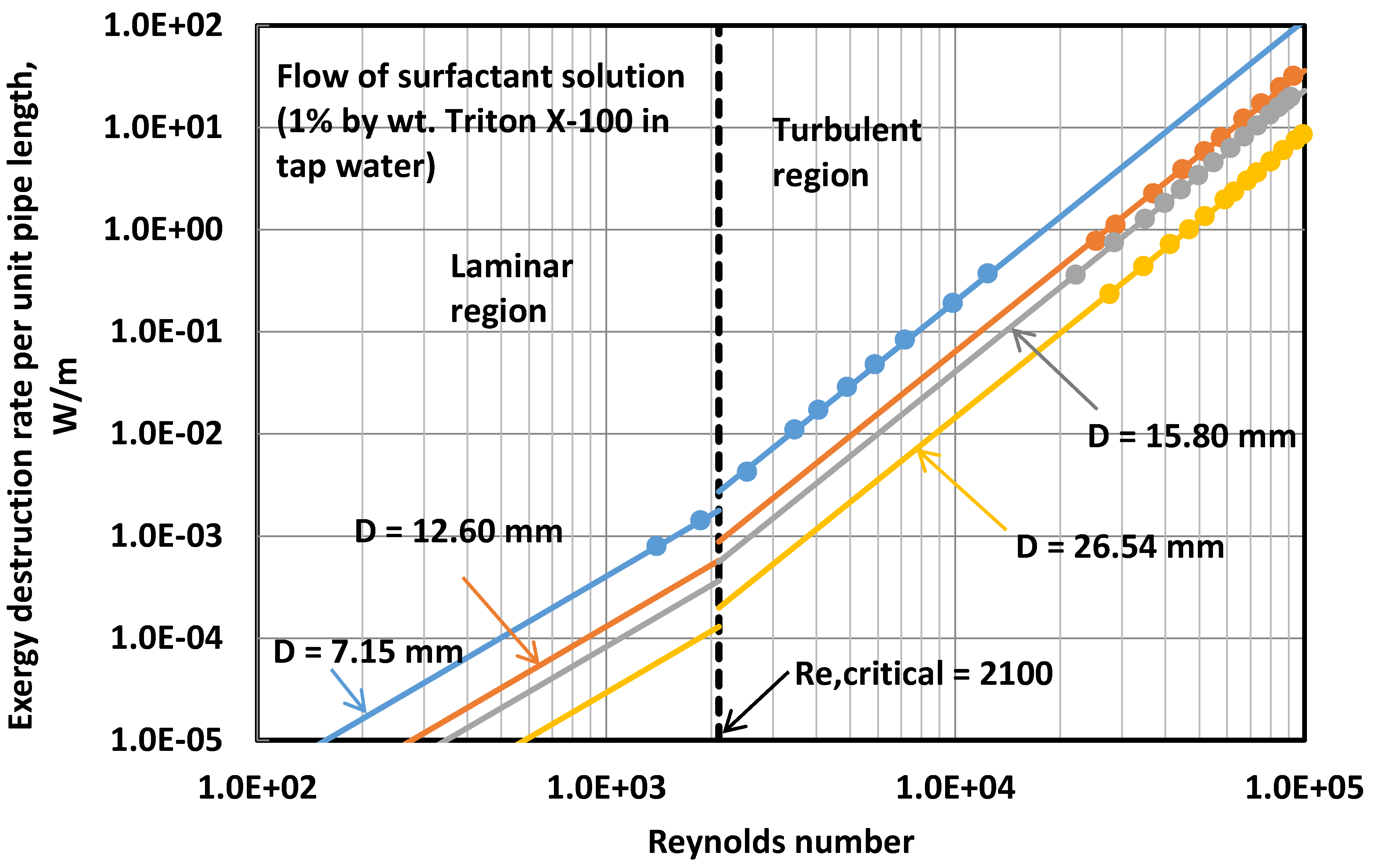
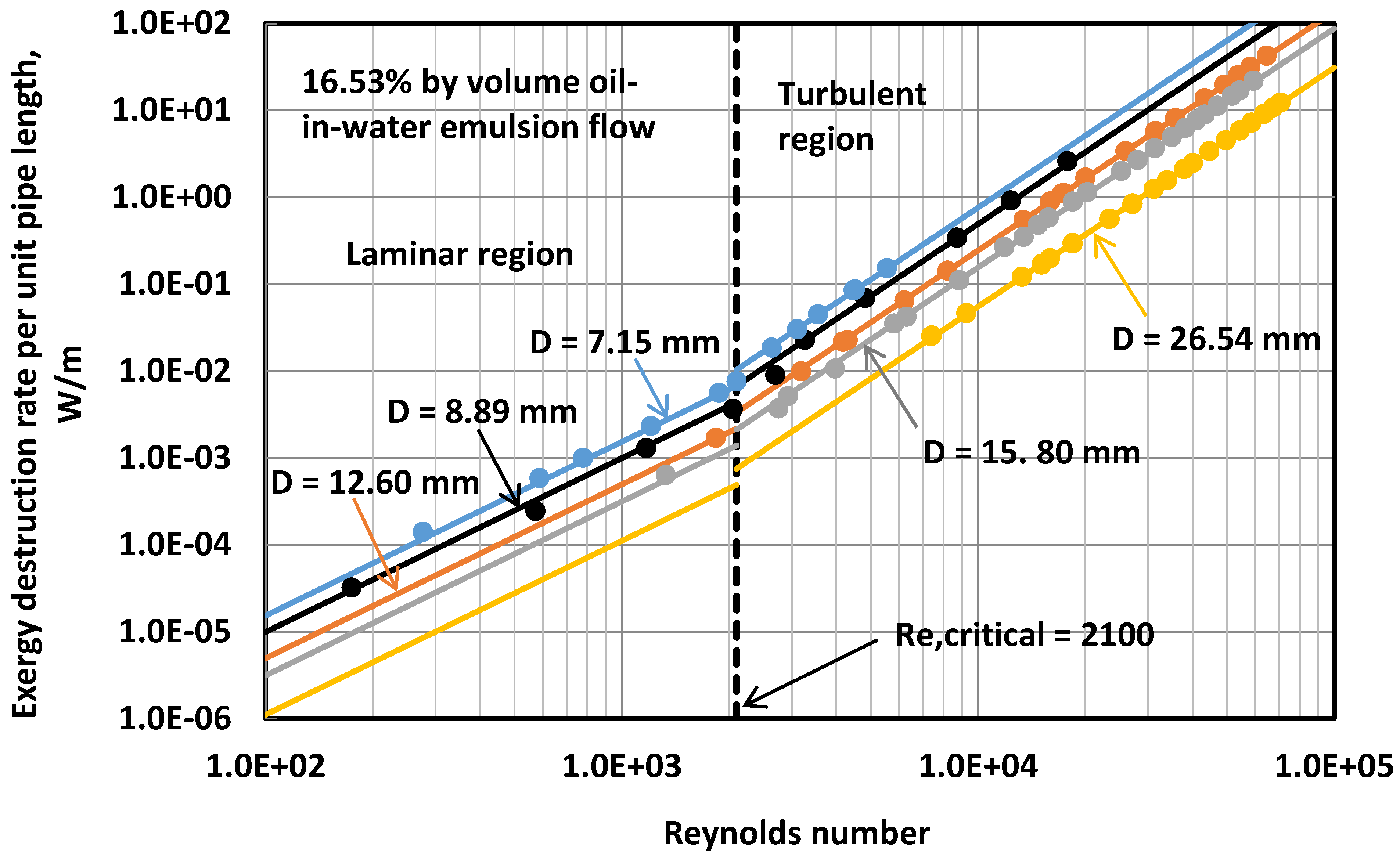
Re range of 3000 to 100,000. Substitution of the friction factor expressions from Equations (18) and (19) into Equation (17) leads to the following relations for exergy destruction in pipe flows:
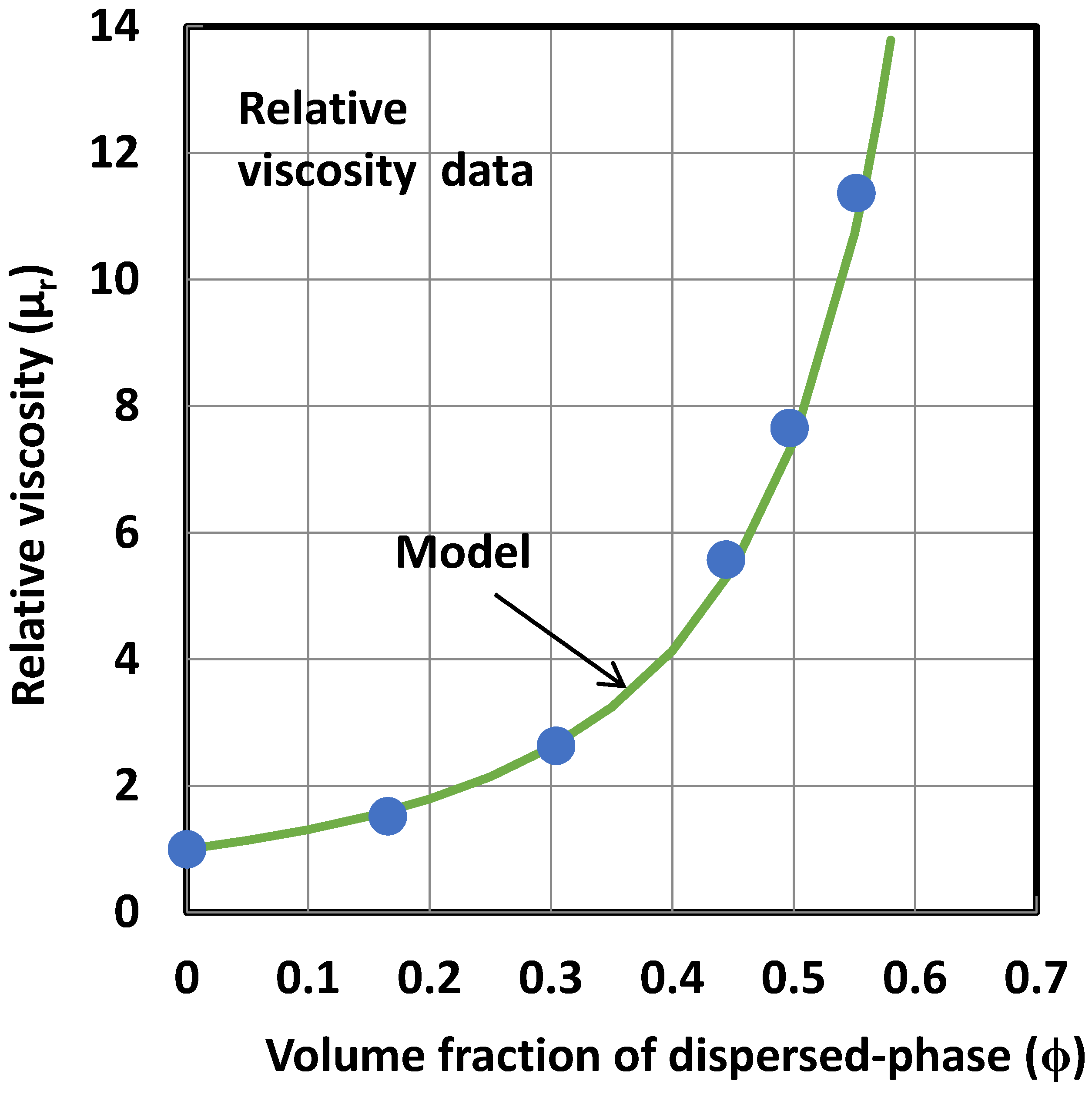
Equations (20) and (21) are predictive models for exergy destruction per unit length in pipeline flow of Newtonian fluids. These models could be applied to pseudo-homogeneous mixtures of two phases such as emulsions of oil and water.
3. Experimental Work
The exergy destruction rates in pipeline flow of surfactant-stabilized O/W emulsions were investigated experimentally in a flow rig consisting of five different diameter pipeline test sections (stainless steel, seamless) installed horizontally. The various dimensions of the test sections are summarized in
Table 1. The pipelines were hydraulically smooth. The hydraulic smoothness of the pipeline test sections was verified by comparing the experimental friction factor
versus Reynolds number data for turbulent flow of single-phase Newtonian fluids (oil and water) with the Blasius equation (Equation (19)). The agreement between the experimental data and the Blasius equation was excellent. The friction factor in turbulent flow of Newtonian fluids is expected to be significantly higher than the prediction of the Blasius equation if the pipe is rough.
Table 1.
Various dimensions of the pipeline flow test sections.
Table 1.
Various dimensions of the pipeline flow test sections.
| Pipe inside diameter (mm) | Entrance length (m) | Length of test section (m) | Exit length (m) |
|---|
| 7.15 | 1.07 | 3.05 | 0.46 |
| 8.89 | 0.89 | 3.35 | 0.48 |
| 12.60 | 1.19 | 2.74 | 0.53 |
| 15.8 | 1.65 | 2.59 | 0.56 |
| 26.54 | 3.05 | 1.22 | 0.67 |
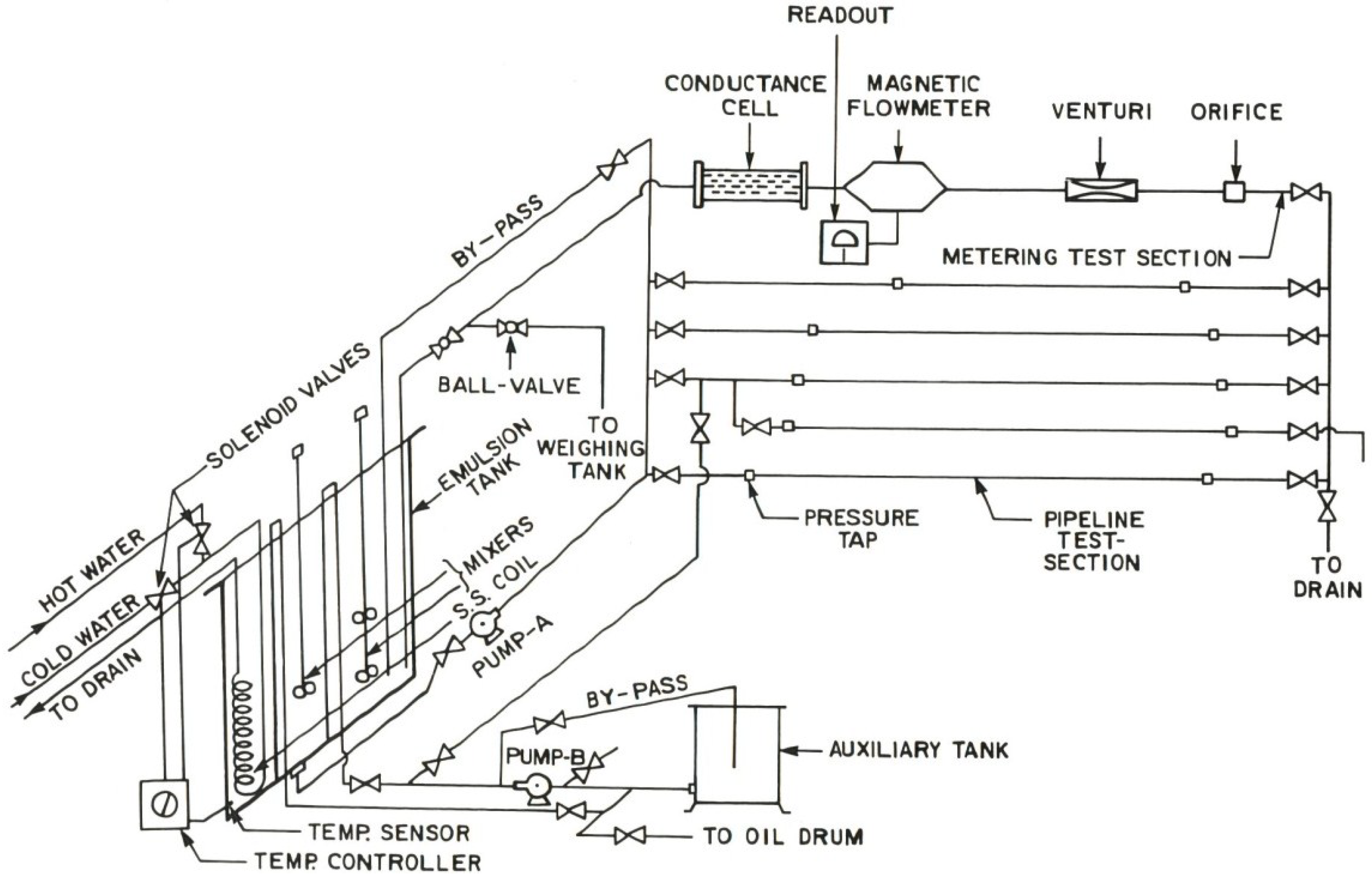
Figure 1 shows a schematic diagram of the flow rig. The emulsions were prepared in a large mixing tank (capacity about 1 m
3) equipped with baffles, two high shear mixers, heating/cooling coil, and a temperature controller. From this tank, the emulsion was circulated to the pipeline test sections, one at a time, by either of the two installed centrifugal pumps.
Figure 1.
Schematic diagram of the flow rig.
Figure 1.
Schematic diagram of the flow rig.
The pump-A (main pump) was used for high flow rates and the pump-B (small pump) was used for low flow rates. Both the pumps had appropriate by-pass arrangements to enable easy regulation of flow rates into the test-section. From the pipeline test section, the emulsion was allowed to return to the mixing tank via the metering section where its flow rate was measured. The metering section included a magnetic flow meter and other devices not used in the present study (orificemeter, venturimeter, and an in-line conductance cell). The magnetic flowmeter was used for the determination of flow rate in the test section at high flow rates; low flow rates were measured directly by diverting the flow outside the flow loop into a weighing tank. The pressure drops in the various pipeline test sections were measured by means of six variable magnetic-reluctance type pressure transducers (Validyne transducers, Validyne Engineering Corp, Northridge, CA, USA) covering a broad range of pressure drop. The output signals from the pressure transducers and magnetic flowmeter were recorded by a microcomputer data-acquisition system.
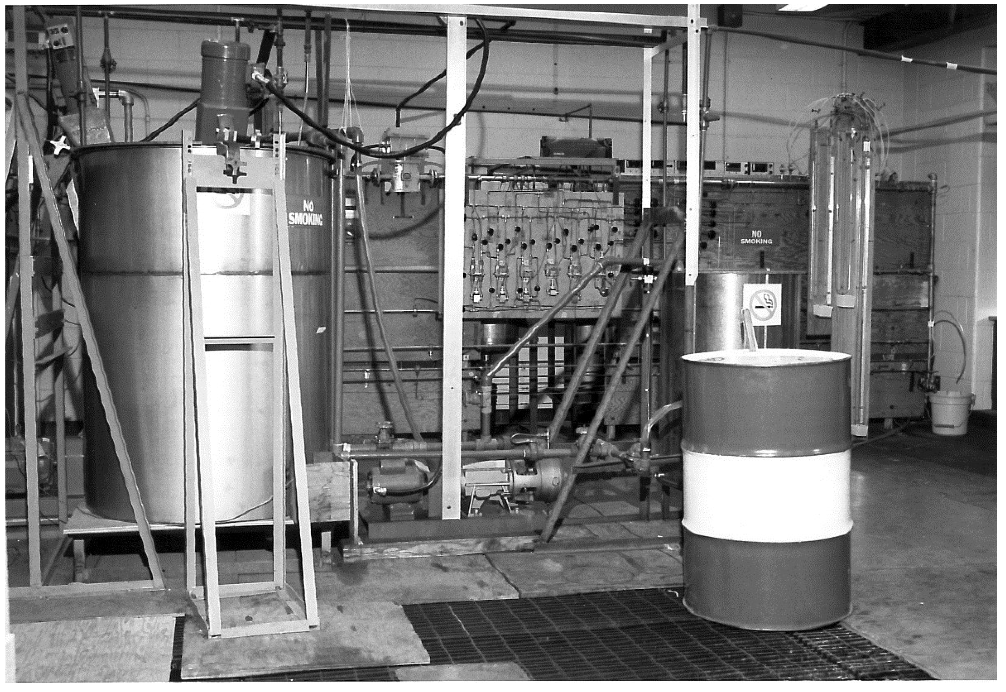
Figure 2 shows the front view of the flow rig.
Figure 2.
Front view of the flow rig.
Figure 2.
Front view of the flow rig.
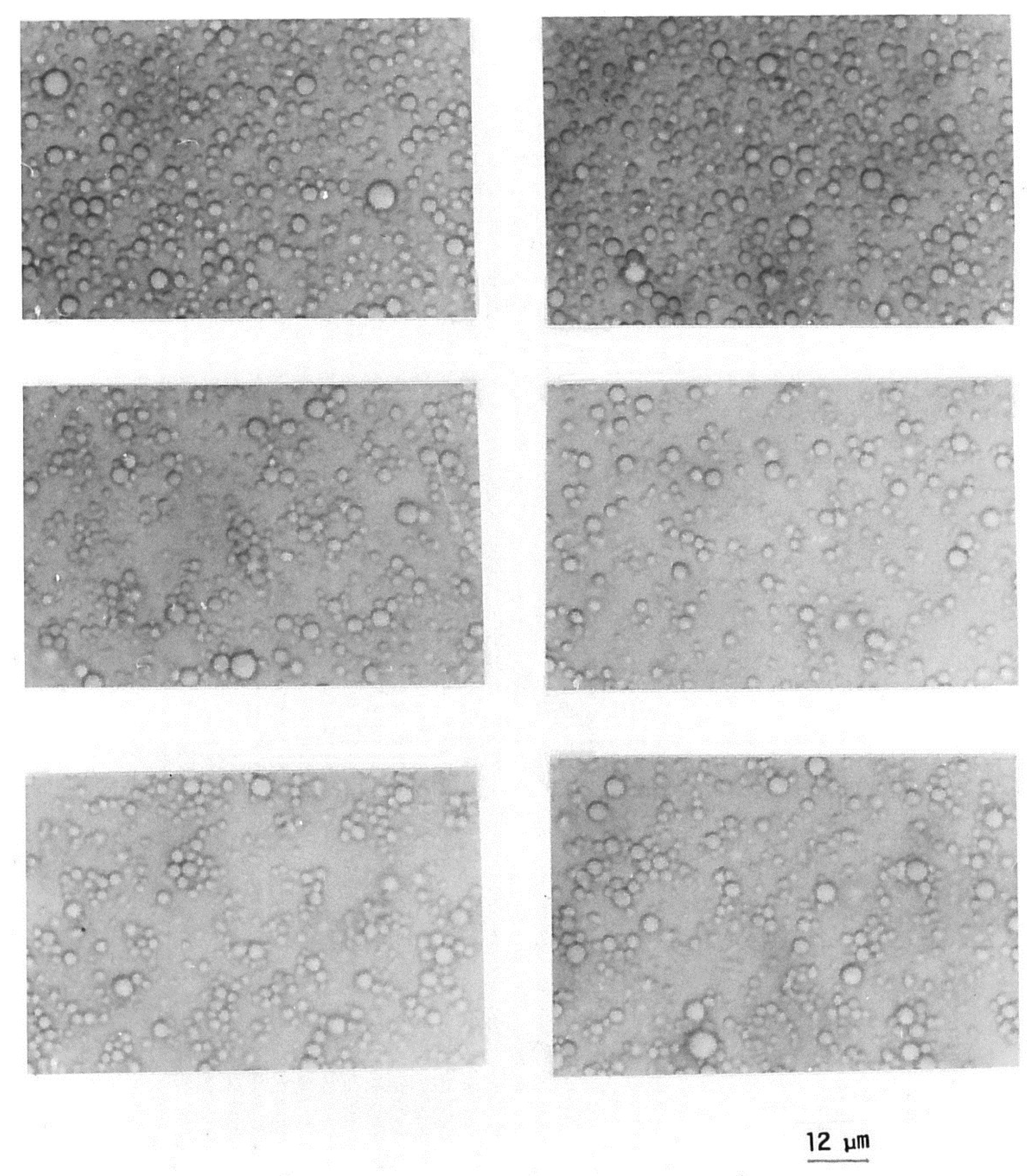
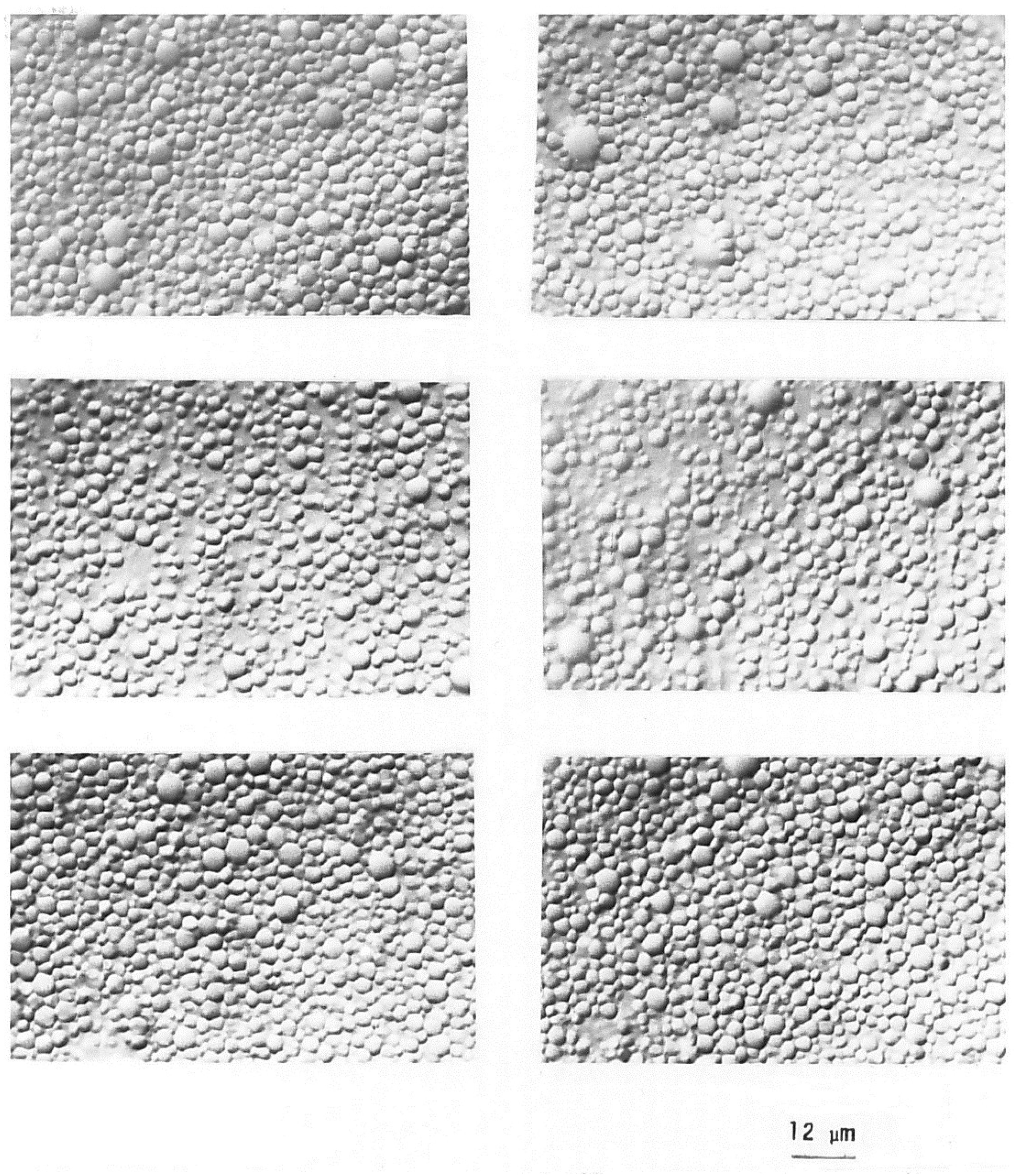
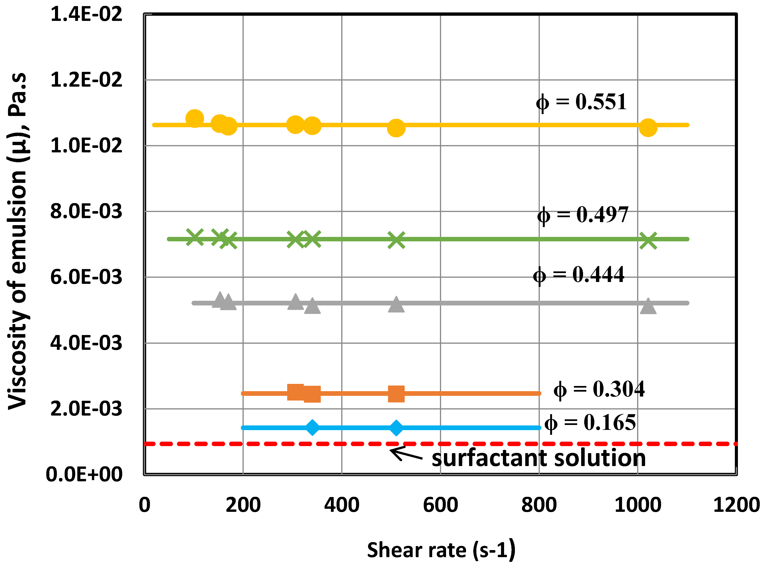
The rheological properties of emulsions were measured in a Fann co-axial cylinder viscometer (Fann Instrument Company, Houston, TX, USA). The emulsion samples were observed under a Zeiss optical microscope (Carl Zeiss Canada Ltd., Toronto, ON, Canada) to obtain information about the droplet sizes. The emulsions were prepared using 1% by wt. surfactant solution in tap water and mineral oil (Bayol-35). The surfactant used was Triton X-100 (isooctylphenoxypolyethoxy ethanol); this is a non-ionic water soluble surfactant. The oil had a density of 780 kg/m3 and a viscosity of 2.41 mPa.s at 25 °C. The experiments were started with aqueous surfactant solution (1% by wt. surfactant) into which a required amount of oil was added to prepare an O/W emulsion. The mixture was sheared in the flow loop for a fixed period of time. To prepare a higher concentration O/W emulsion, more oil was added to an existing emulsion. The experimental work was conducted at a constant temperature of 25 °C. The temperature was maintained constant in the flow loop with the help of a temperature controller installed in the mixing tank.


