Abstract
Economic analysis and market simulation tools are used to evaluate uranium (U) supply shocks, sale or purchase of uranium stockpiles, or market effects of new uranium mines or enrichment technologies. This work expands on an existing U market model that couples the market for primary U from uranium mines with those of secondary uranium, e.g., depleted uranium (DU) upgrading or highly enriched uranium (HEU) down blending, and enrichment services. This model accounts for the interdependence between the primary U supply on the U market price, the economic characteristics of each individual U mine, sources of secondary supply, and the U enrichment market. This work defines a procedure for developing an aggregate supply curve for primary uranium from marginal cost curves for individual firms (Uranium mines). Under this model, market conditions drive individual mines’ startup and short- and long-term shutdown decisions. It is applied to the uranium industry for the period 2010–2030 in order to illustrate the evolution of the front end markets under conditions of moderate growth in demand for nuclear fuel. The approach is applicable not only to uranium mines but also other facilities and reactors within the nuclear economy that may be modeled as independent, decision-making entities inside a nuclear fuel cycle simulator.
1. Introduction
Unlike other commodities, natural uranium is not traded on an organized commodity exchange market. The uranium market mainly works on fixed long term supply contracts based on direct negotiations between uranium mine operators and facilities. Contract pricing can be indexed to a single fixed price, but is more commonly based on various reference prices with economic corrections built in. The corrections are tied to the spot market price, which is based on current supply and demand and subject to speculative effects. Approximately 80% of all uranium has been sold under long term contracts and 20% of all uranium by spot market price [1,2,3]. The objective of this work is to extend an existing market clearing model of the uranium and enrichment industries [4]. This model analyzes the impact of new technologies as well as inventory management policies on the uranium market. The work presented here introduces individual firm decision making as well as friction to the existing equilibrium supply/demand model. Each firm (uranium mine) makes decisions based on its own capital and fixed and variable operating costs, and opening as well as short- and long-term shutdown decisions are taken based upon current as well as projected future market conditions.
A summary of the market clearing model of the uranium and enrichment industries follows. It is built around databases of primary and secondary uranium supply [5]. The model is built as a time-dependent simulation that determines the uranium and enrichment market conditions by calculating the intersection between the supply and demand curves in each user defined time period of the simulation (typically, annually). At each time step, U and enrichment market clearing states are solved; hence the model responds to shifts in supply and demand, for instance closure of a major mine.
Since nuclear reactors require many years to modify their demand for low enriched uranium (LEU) fuel, the LEU requirement per unit of installed nuclear capacity is treated as fixed, but utilities can substitute natural uranium (NU) for enrichment services, so the model’s uranium and enrichment demand curves exhibit considerable short run price elasticity while still meeting LEU requirements. Each demand curve is a locus of cost-minimizing tradeoffs between uranium and enrichment services over the range of feasible production levels of those commodities.
The supply curves are made from the available information in the uranium mine and enrichment plant databases, and the NU supply curve is augmented by secondary sources of uranium which are generally assigned zero production cost. It is important to note that this model is not used to predict prices, but instead to evaluate the market impact of inventory sales strategies and other policy measures.
As mentioned, this paper focuses on the addition of a key feature to the market-clearing model, namely the ability of individual uranium mines to react to short run changes in the U market price. This capability is important in the context of nuclear fuel cycle (NFC) simulators which depict entities including not only uranium mines but also other nuclear fuel cycle facilities and reactors. These simulators must be able to realistically model the behavior of entities given that they are profit maximizing and make rational decisions to begin or continue operating, as well as to shut down when conditions warrant it. Therefore, the chief purpose of this paper is to demonstrate autonomous decision-making by individual entities within a simulation of part of the nuclear fuel cycle.
In the augmented market model, each uranium mine acts like an individual agent that is capable of deciding under which conditions it is economical to continue operation, suspend U mining or open a new uranium mine. Decisions are partly based on the current time period U market price: for instance, if the price exceeds a prospective mine’s total operating costs, the model opens the mine. To make these decisions, the model must have additional information about U mine’s economic characteristics, specifically its total overnight capital cost (TOC) of construction, operation and maintenance (OM) and decommissioning (DD) costs. Since these are generally not available for individual mines, a method for estimating them from available unit cost data is presented. This treatment of mine opening and re-opening decisions is a simplification of a lengthy and involved process. Companies planning to operate mines must undertake a complex licensing process and provide the regulator with a long term financial management and decommissioning plan. In case of unexpected closure, the mine owner must obtain license renewal prior to re-opening [6].
Since the simulator marches forward in time, individual agents make decisions not knowing what others are doing and based only upon conditions in the current time step. Since this gives rise to unrealistically myopic behavior, a time rollback function has been implemented to allow the simulator to move back in time in order to change agent decisions. This rollback function simulates the ability of entities to make long-run market predictions and forecasts; by rolling back the simulation clock to change a decision, an agent is modifying its strategy based upon the projected evolution of the market and the future actions it expects other entities to take. In this implementation, marching backward and forward in time creates a simulation strategy where uranium mines operate throughout their lifetimes rather than, say, shut down early due to over-construction of capacity. To implement the rollback decision function given data limitations, each mine operator operates under an identical set of decision criteria. In reality, individual uranium mines will possess unique resources and financial positions and thus will react differently in the face of market fluctuations.
The methodology section of this paper describes three steps that are carried out to implement the market model:
- Create short run supply curves for each mine (Section 2.1);
- Aggregate the individual uranium mine supply curves into the short run market supply curve (Section 2.2);
- Go through each mine’s decision making process (begin operating, continue operating, shut down) (Section 2.3).
Once the methodology is developed, two cases are presented in Section 3, Results. The first includes five made-up mines and is purely illustrative of the model’s behavior. The second implements the realistic depiction of the world uranium and enrichment markets described in [4].
2. Methodology
The work presented here builds upon the market clearing model of the uranium and enrichment industries described in [4]. That model is built upon databases of primary and secondary uranium resources as well as enrichment facilities, with each enrichment facility having a unique cost structure. The model derives market-clearing conditions by locating the intersections between the annual supply and demand curves for uranium and enrichment services while also considering the effects of secondary supplies including highly enriched uranium down blending and sale of natural uranium inventories. Therefore, the model incorporates the coupling between the uranium and enrichment markets. For instance, an increase in uranium prices will lead to decreased tails assays, more demand for enrichment, higher enrichment prices and ultimately reduced demand for natural uranium.
Each mine in the simulation has unique characteristics including total uranium reserves, earliest feasible opening date, capital and operating costs and others detailed below and in [4]. Since these characteristics are fixed, the supply curve for each individual mine is also the same in every time period as long as the mine still possesses uranium reserves it can produce. Therefore the production decisions of each mine can be determined based on the short-run market price, which is in turn set by the industry short run supply curve aggregated over all mines that are able to produce in that time period. The aggregated short run industry supply curve displays all uranium mines which can potentially produce in a given time period if the price is high enough.
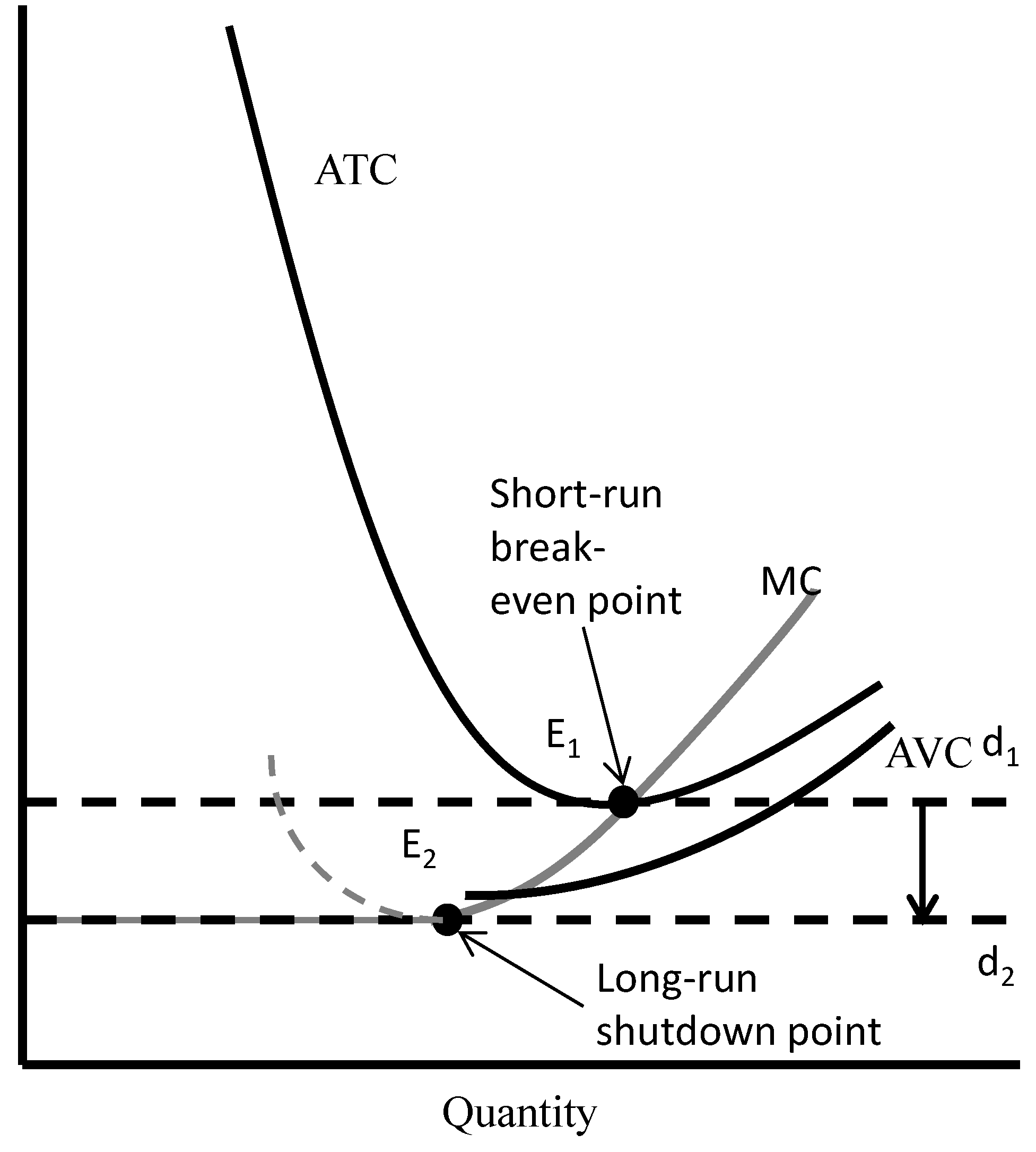
Figure 1 distinction between an individual mine “shutting down” in the short run and “exiting” price in the long run. Figure 1 follows the economic rules, which are described in [7]. The marginal cost (MC) is the variable cost incurred by producing one additional unit of output. The average variable cost (AVC) is the average value of the MC for all units of output produced. The average total cost (ATC) is the AVC plus the amortized capital cost (ACC) divided by the number of units of output. For a mine to operate, its economic costs must be covered. The MC curve crosses ATC at its lowest point (E1) because the MC is of producing an additional unit of output is averaged into the ATC. When the MC is less than the ATC, each new unit of output lowers the ATC. A new mine will not begin to operate unless its average total cost of producing uranium is less than or equal to the mine’s MC. This point is known as the short-run breakeven point (E1 in Figure 1). If a mine is currently operating it will continue to operate until the market price drops below the minimum value of its AVC. This is known as the long-run industry exiting point (E2).

Figure 1.
Cost curves for a single uranium mine.
Figure 1.
Cost curves for a single uranium mine.
2.1. Short Run Individual Mine Supply Curve
The original model’s database does not include information about capital, operation and maintenance or decommissioning costs for individual uranium mines, only their unit cost of uranium production at a reference output level. Operating cost information is required to allow the simulator to make short run operation decisions, while capital costs become relevant when determining whether to open or decommission a mine. Disaggregated capital, operating and decommissioning cost data is available from WISE Uranium Project for a limited number of mines [8].
One representative mine of each type, underground (UG), open pit (OP) and in situ leach (ISL), is chosen from this data set. The Generation-IV Economic Modeling Working Group (EMWG) unit cost calculation procedure is used to compute unit production costs—UC ($/kg U), for these mines [9]. All other mines of that type are assumed to adhere to the same relative distribution of capital, operating and decommissioning costs. Hence these costs are obtained by scaling the costs for the reference mine by the ratio of unit costs, as detailed below. This simplification was made in response to the unavailability of detailed cost structure breakdowns for individual mines. The representative disaggregated costs available in [8] are used in this paper in order to demonstrate the implementation of the model.
Table 1 provides the reference data set for each mine type. The methodology for relating TOC, OM, and DD to UC is described next. The unit cost, UC, is calculated from:
Where M: Annual production (throughput) of product in kg of basis unit/yr; technology-specific basis unit may be U, SWU (separative work unit), etc. ADD: Amortized annual decommissioning costs.
The unit cost components are calculated as above. The amortization factor (AF) is given by:
where r: Real discount rate, T0: Duration (years) of operation.
A sinking fund amortization factor (SFF) with a lower rate of return applies to decommissioning costs. It is calculated from:
where rSF: Real sinking fund rate, T0: Duration (years) of operation. Then TOC, IDC (interest during construction) and DD are calculated from the reference data:
where Tc: Duration (years) of construction.
The next step is to calculate the scaled costs for other mines of the same type. In the discussion that follows, variables subscripted “r” apply to the reference mine of a given type (OP, UG, ISL). Unsubscripted quantities apply to another mine of the same type. The amortized annual capital, OM and DD costs and interest during construction are scaled from reference values as follows:
The OM, is interpreted as the AVC at the reference annual production level, M. In reality, individual mines would increase or curb production as conditions warranted; however the existing model [4] permits mines to function at their reference capacity or not at all. By formulating a mine-specific supply curve, the modification described next enables each mine to select its own production level at every time step.
A bottom-up engineering cost analysis would be needed to construct such a supply curve. Since the objective of this work is to demonstrate a method for making use of such data in a simulation, a plausible functional form was chosen to represent a generic short run supply curve, which shows the quantity supplied by individual U mine at certain price level. The form chosen is quadratic, as was proposed in [10]. It is and given by:
where Q: supply quantity in given period (usually one year), P: marginal cost of supplying an additional unit at quantity Q; a, b, c: coefficients to be determined.
For each uranium mine, the existing database from [2] provides a reference capacity (tonnes of uranium produced per year) and a reference production cost ($ per kilogram of uranium produced), from which is calculated marginal cost of supplying. Therefore, to determine the coefficients a, b, and c the following criteria are imposed:
Here Q1 and P1 are the reference capacity and cost from the database. Economic theory provides that a firm’s short run marginal cost curve exhibits a U shape, as predicted by Equations (12). The shape arises because costs per unit of production first decrease as production rises from very low levels and scale benefits are realized. As additional capital and labor inputs are applied to increase production, though, the marginal benefit of these inputs begin to decline as they outstrip the ability of a firm’s infrastructure to effectively use them. Although there exists insufficient historical mine data to calibrate the marginal cost curve, the U shape of Equations (12) provides the correct type of feedback to the cost model. The point P2 = 0.5P1 and Q2 = 0.7Q1 the marginal cost of mining an additional unit of uranium is assumed to reach its lowest value, 70% of the reference cost P1, when the mine’s production stands at half of the reference level Q1.
The individual mine supply curve is the upward sloping part of the marginal cost curve (the part above the average cost curve). The portion of the marginal cost curve above ATC (Figure 1) is a profit maximizing individual mine supply curve. Portions of the marginal cost curve to the left of the shut-down point (E2) are not part of the short run supply curve, because to produce on the left side of the E2 MC costs increase (dashed line in Figure 1) and ATC costs significantly increase. Operation in this part of the MC curve is uneconomical.

Table 1.
Reference data for costs calculation from the WISE Uranium Project Calculators.
| Reference U mines | Type | UG | OP | ISL |
|---|---|---|---|---|
| Data from [3]: | TOC, $ | 2.81 × 10⁸ | 3.47 × 10⁸ | 1.11 × 10⁸ |
| OM, $/yr | 1.04 × 10⁸ | 1.62 × 10⁸ | 1.73 × 10⁷ | |
| DD, $ | 3.39 × 10⁷ | 5.92 × 10⁷ | 2.86 × 10⁷ | |
| M, kg/yr | 7.72 × 10⁵ | 3.16 × 10⁶ | 4.12 × 10⁵ | |
| Calculated from data following procedure in text | ACC, $/yr | 4.25 × 10⁷ | 7.93 × 10⁷ | 2.67 × 10⁷ |
| ADD, $/yr | 1.07 × 10⁶ | 5.78 × 10⁶ | 3.07 × 10⁶ | |
| IDC, $ | 4.36 × 10⁷ | 5.37 × 10⁷ | 1.72 × 10⁷ | |
| UC, $/kg U | 192 | 77.9 | 114 |
2.2. Short Run Market Supply Curve
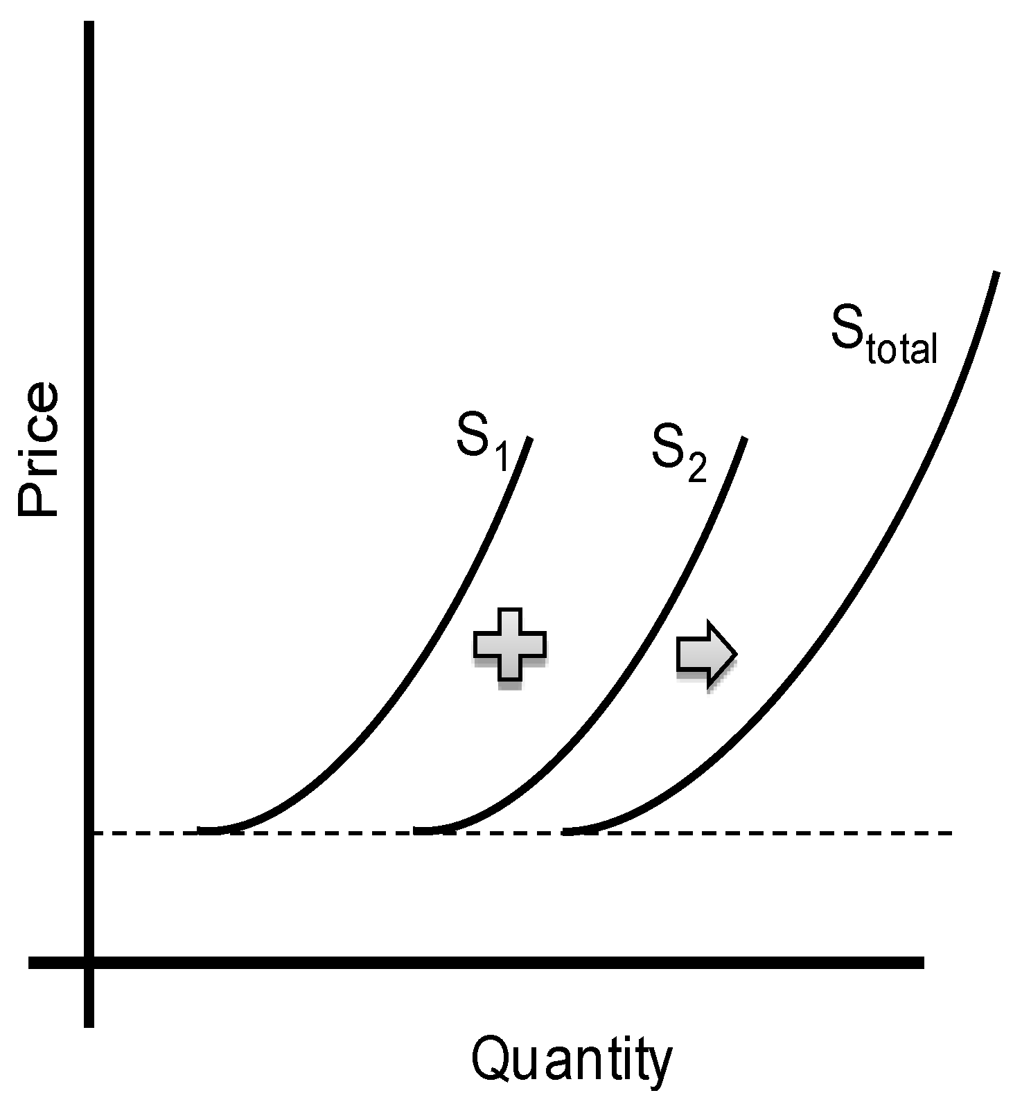
The short run market supply curve is defined as the horizontal sum of the individual mines’ supply curves, so that the amount that would be supplied Q by all agents at a price level p is:
where n: number of U mines,
: supply curve of firm i from Equation (11). Construction of the supply market curve shown in Figure 2.

Figure 2.
Uranium market supply curve creation.
Figure 2.
Uranium market supply curve creation.
2.3. Short-Run Decision Making Process
During each year of the simulation the market clearing model uses the decision criteria summarized at the beginning of this section to determine whether each mine will operate. It then must decide how much uranium the mine will contribute to the total amount supplied across the industry. The model simulates the uranium market for each year of the simulation using the following scheme, starting with the first year of the simulation (t = 1) and running through the last year, t = T. This loop is visualized in Figure 3:
- The supply curve is drawn by finding the amount supplied as a function of price. To begin, the market price is set to 0.
- The secondary supplies are added to the supply curve.
- The offer loop is performed for the set price. In this step the model determines which mines are operating and how much material they are producing. The offer logic is described below.
- The total amount suppliable from the available mines in current time period at the set price level is summed to determine the cumulative supply.
- A check is performed to see if the current model price is equal to a user-specified maximum modeled price.
- If the market price equals the maximum, proceed to step 6.
- If the market price is not yet equal to the maximum price, the market price is increased by a small user-specified increment and returned to step 2 above.
- The supply curve is now drawn. The uranium demand curve for the time step is next drawn using methods that were described in [2].
- The intersection of the supply and demand curves is found and determines the market price for the time step.
- The mine reserves are updated by deducting the offered amount (quantity supplied at the market price) from each mine currently operating.
- The current time of the simulation is checked against the value of the simulation end time (T).
- If t < T, time is incremented by one year and the loop restarts.
- If t = T the simulation ends.
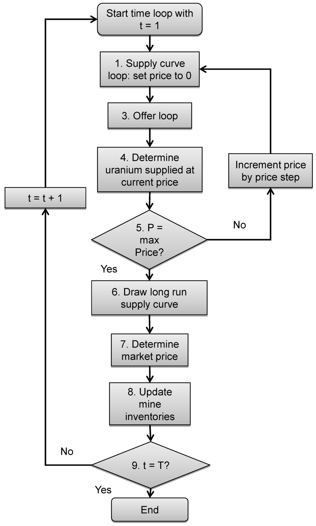
Figure 3.
Main time loop algorithm.
Figure 3.
Main time loop algorithm.

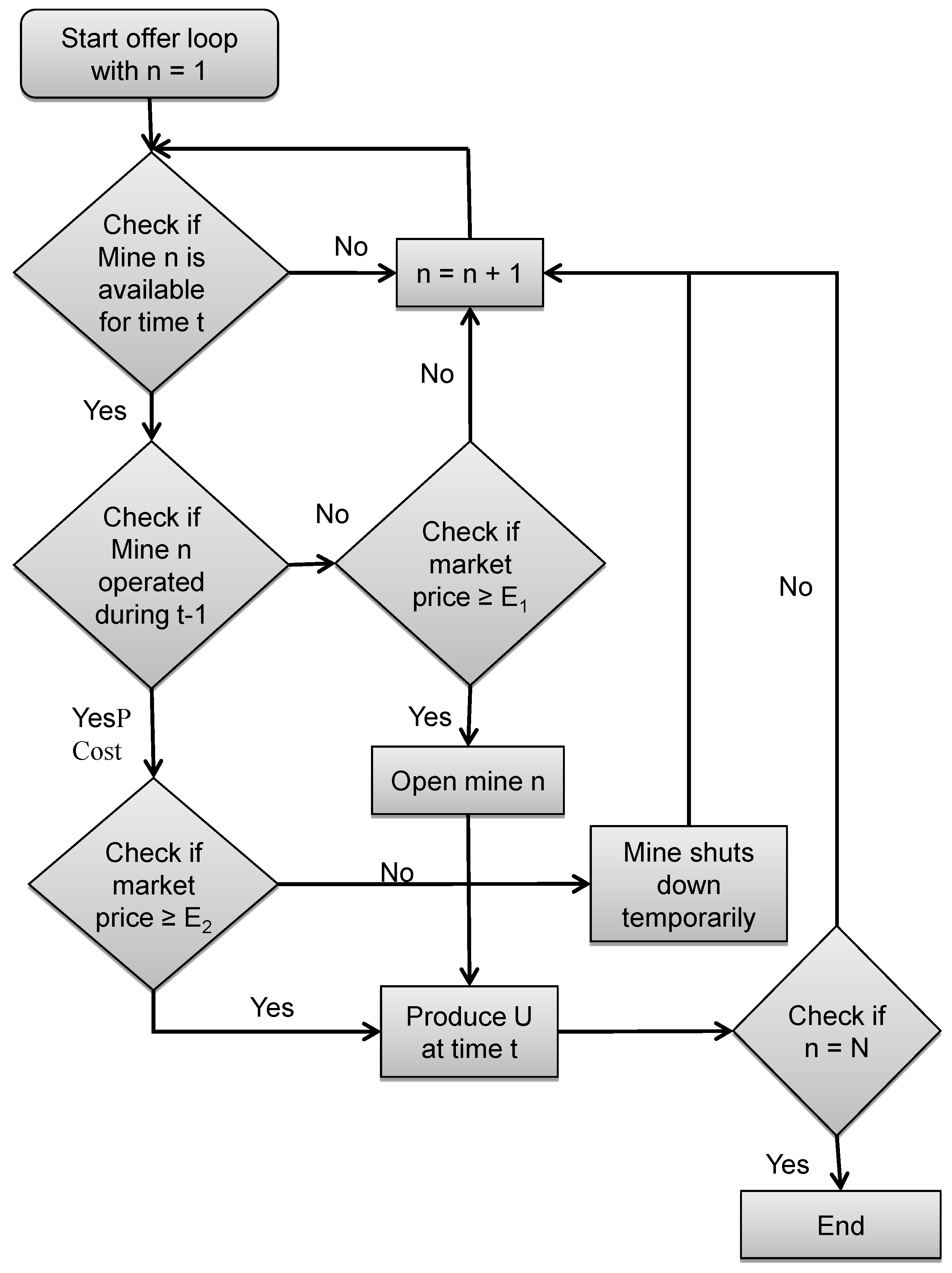
Inside the offer loop, the following operations are performed for each mine in the simulation, starting with the first mine (n = 1). The loop is visualized in Figure 4:
- The mine is checked for availability. Any mine not currently able to operate in the given year is unavailable.
- If the mine is not available, skip to the next mine.
- If the mine is available, proceed to step 2.
- The mine is checked for operation in the previous time step.
- If the mine operated in the previous time step, go to step 3.
- If no uranium was produced by the mine in the previous time step, proceed to step 4.
- The E2 of the mine is check against the current market price.
- If E2 is greater than or equal to the market price proceed to step 5.
- If E2 is less than market price the mine enters temporary shutdown and the model restarts at step 1 with the next mine.
- If the mine did not operate in the previous time-step, the current market price is checked against the mine’s E1.
- If E1 is greater than or equal to the market price, a new mine is opened and the model proceeds to step 5.
- If E1 is less than the market price, the loop restarts with the next mine.
- The mine is flagged to produce uranium during the current time step.
- A check is made to determine if the current mine is the last mine in the simulation (n = N).
- If true, the loop ends.
- If false, the loop is restarted with the next mine in the list.

Figure 4.
Uranium mine decision making event chain.
Figure 4.
Uranium mine decision making event chain.
3. Results
3.1. Test Case Conditions
The test case is designed to illustrate the decision algorithm for a simple scenario characterized by a limited number of uranium mines and constant low-enriched uranium (LEU) demand. The simulation runs from 2010 to 2030 under a fixed annual reactor fuel demand of 6790 t/year of 4.5% enriched U and 3390 t/year of natural U to supply Canada Deuterium Uranium (CANDU) and other NU-fueled reactors. These values are representative of world reactor fuel demand in 2010 and will be used again in the next section when a full-scale scenario of world production and demand is presented. As additional simplifications for this test case, the enrichment price is fixed at $100/SWU and no secondary supplies of U are made available. Table 2 contains information about total reserves, annual U extraction rate, production costs, year from which each mine is available to enter production and mining method.
The simulation test case aims to demonstrate:
- 1
- mine opening decisions based on market price;
- 2
- the effect of supply capacity changes on short and long run market prices;
- 3
- competition effects where a lower-cost U mine becoming available displaces other U mines from the market.
Table 2 lists the properties of the five mines included in the demonstration case. Recall that the uranium production cost table entry is the cost, in $/kgU, if the mine produces at its reference annual extraction rate. The amount actually produced every year by each mine depends on the market-clearing price as described in the previous section. In this test case, mine E is a large and inexpensive U producer with a production cost of 50 $/kgU at its reference capacity 30,000 tU/year. Unlike the other mines, mine E has a large uranium reserve that will not be exhausted during the 2010–2030 period. Of the other mines, A, B and C feature progressively higher costs and will open in succession if demand warrants it. Mine D cannot open earlier than 2018, but its low reference production cost, 60 $/kgU, may cause the U market price to decrease and might push some other U mine out of the market.
Table 2.
Primary uranium supply data.
| U mine | Total Reserves & Resources tU | Reference Annual Extraction Rate tU/year | Year Available | Reference Cost $/kg U | Mining Method |
|---|---|---|---|---|---|
| A | 150,000 | 15,000 | 2009 | 75 | ISL |
| B | 300,000 | 15,000 | 2009 | 100 | ISL |
| C | 200,000 | 20,000 | 2009 | 120 | UG |
| D | 150,000 | 15,000 | 2018 | 60 | ISL |
| E | 10,000,000 | 30,000 | 2009 | 50 | UG |
To illustrate the sensitivity of the results to the shape assigned to the individual supply curves, the test case is carried out for three values of the (P2, Q2) lowest-cost production point which was described in Section 2.1. The Q value is the quantity at which the marginal cost of producing the next unit is minimized, while P is the marginal cost at that quantity. Table 3 lists the P2 and Q2 values studied. They are normalized against the reference cost and quantity respectively, so that P2 = 0.5, Q2 = 0.5 means that the mine’s marginal cost is minimized at 50% of its reference production level, and at that level its MC is 50% of the reference value. Hence changing the P and Q coefficients alters the slope and shape of the supply curve as shown in Figure 5. The steeper the supply curve for Q > 1, the costlier it is for the mine to produce additional uranium beyond its reference annual capacity. This reflects the need to make short term investments in additional equipment and labor.
Table 3.
Individual supply curve coefficients.
| No. | Q2 | P2 |
|---|---|---|
| 1 | 0.8 | 0.5 |
| 2 | 0.7 | 0.5 |
| 3 | 0.5 | 0.5 |
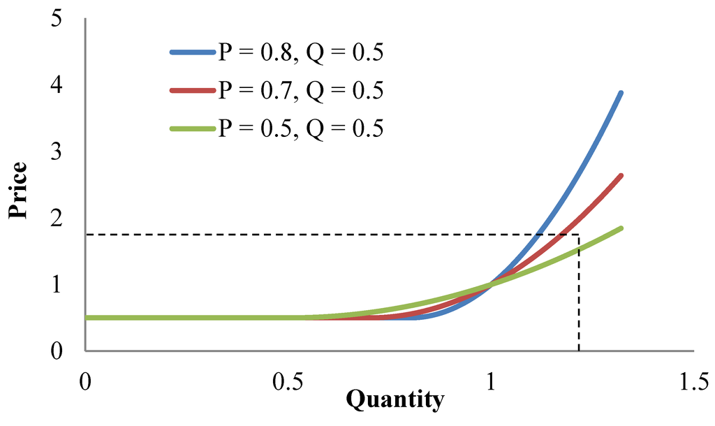
Figure 5.
The individual supply curve with different coefficients.
Figure 5.
The individual supply curve with different coefficients.

3.2. Test Case Results
Figure 6a–c shows the uranium supply mix for the three supply curve calibrations presented in the test case. The general trends are similar: the two lowest-cost mines, A and E, initially provide all supply. In order to do so, they both produce somewhat more uranium than their reference capacity annually. Figure 7 shows the uranium price evolution for each calibration. It can be seen that the uranium price is initially above $75/kgU, the reference production cost for mine A, for all three calibrations. However, only for the steepest calibration (P = 0.5, Q = 0.8) does mine B enter into production as well. This is because at this calibration mines A and E cannot increase production far beyond their design values without incurring sharply increasing costs. Therefore, in this case mine B can profitably enter into production if it produces somewhat less uranium than its reference capacity (hence at somewhat lower than its reference $100/kg U cost).
Regardless of calibration, in 2018 low-cost mine D becomes available and is entered into production. This causes the price of uranium to drop, but not so far as to drop below mine A’s long term shutdown price. Therefore, A continues to operate until its supply is exhausted. For the case where mine B had already entered the market, though, it chooses to enter short term shutdown when mine D opens. Only after mine A is exhausted does it become feasible for B to again enter the market. In all cases, after D is exhausted, the market clearing price rises as mines B and E are operating since B has substantially higher costs than D.
This demonstration case illustrates the effect of the individual firm supply curve elasticities. It is possible to affect firms’ decision-making by modifying their supply curves. The original model of [4] was inflexible in the sense that each mine could only produce at its reference capacity and cost. This misses the flexibility mines have to respond to changes in price by expanding or reducing production. Although not evident from the plots, the rollback algorithm prevented mine “C” from opening shortly before inexpensive mine “D” became available in 2018. Mine “C” features somewhat higher operating costs than “B” but would have been profitable had “D” not appeared. Instead, mine “C” elected not to open and mine “B” continued to meet all demand until “D” opened.
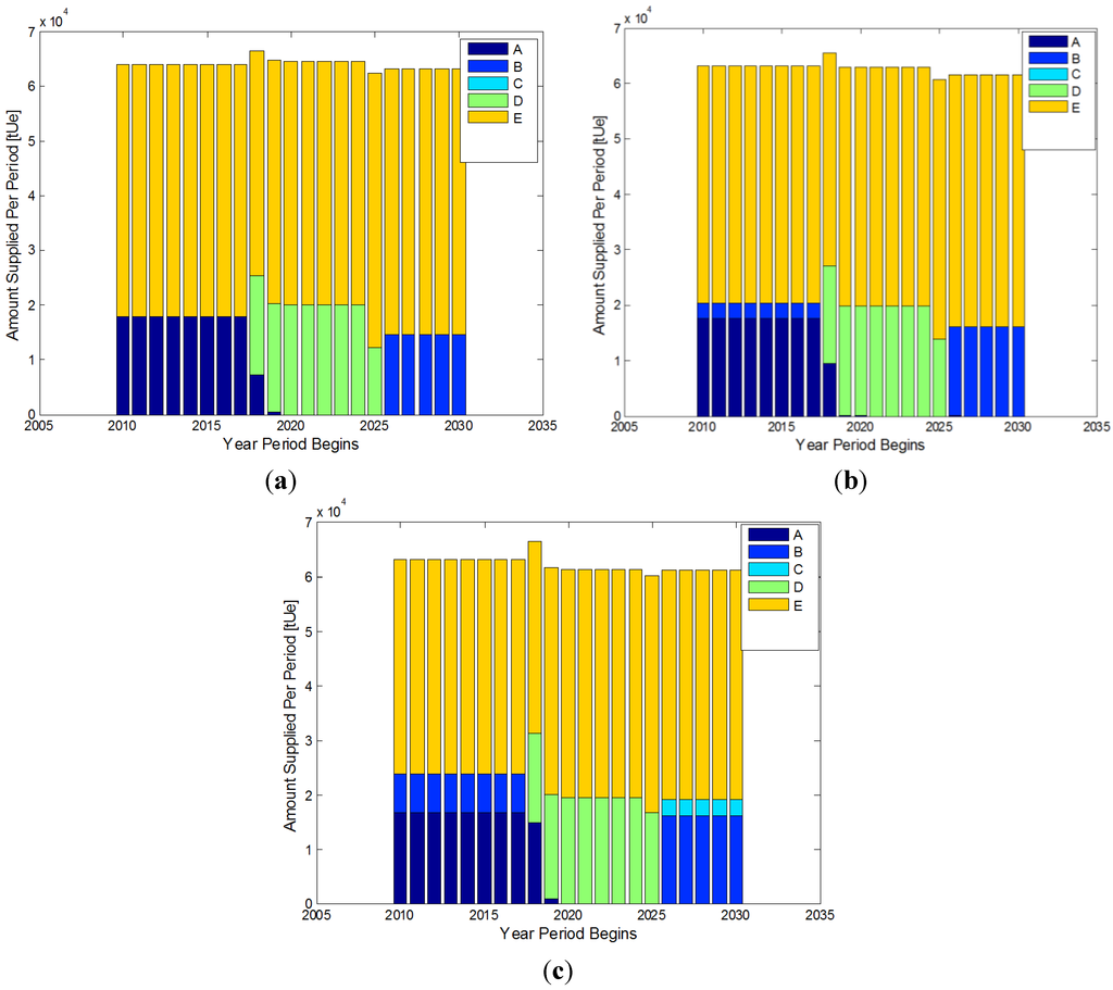
Figure 6.
Amount supplied per period with coefficients: (a) Q = 0.5, P = 0.5; (b) Q = 0.7, P = 0.5; (c) Q = 0.8, P = 0.5.
Figure 6.
Amount supplied per period with coefficients: (a) Q = 0.5, P = 0.5; (b) Q = 0.7, P = 0.5; (c) Q = 0.8, P = 0.5.
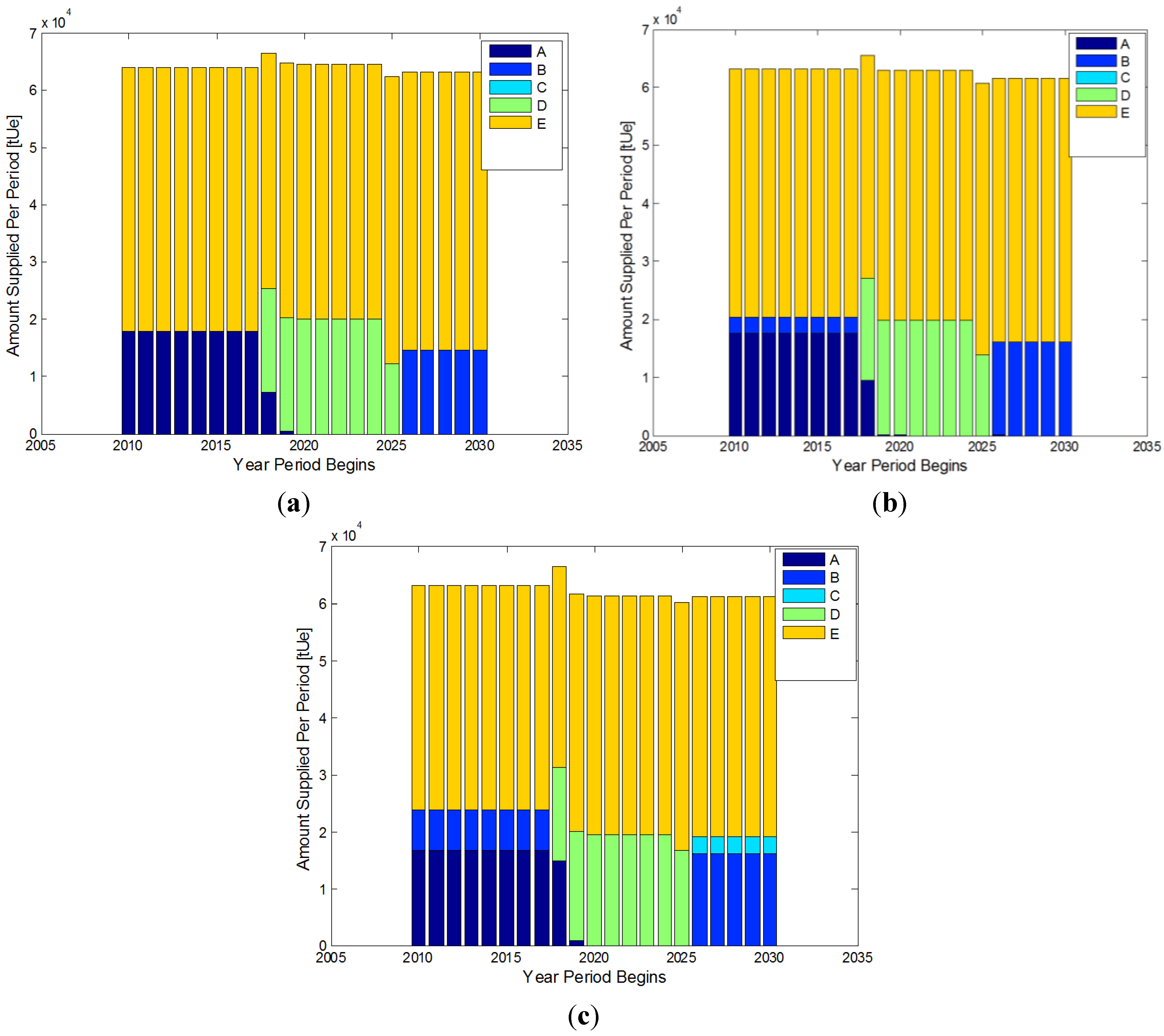
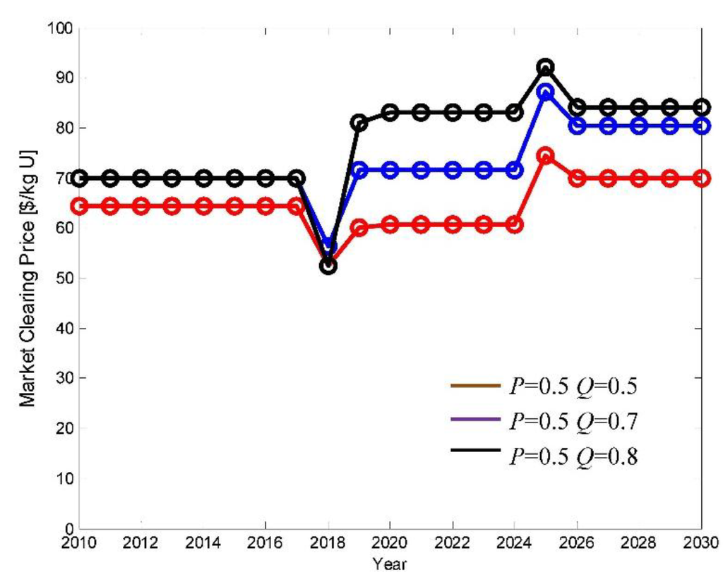
Figure 7.
Market clearing price.
Figure 7.
Market clearing price.

3.3. World Case Conditions
The world case scenario utilizes the reference-case uranium and enrichment industries described in [4] and summarized here. As Table A1 shows, the reference scenario does assume that weapons grade plutonium (WGPu), down blended HEU, and stocks of natural uranium will be available as secondary sources of supply and that re-enrichment of stored depleted uranium continues. Other global parameters used in the reference scenario are given in Table A2. This case assumes a 2.6% annual LEU fuel demand growth from its 2010 value. Enrichment plant capacities follow the schedule given in Table A3; in addition, all enrichment plant capacities are assumed to grow at a rate equal to that of LEU demand, an average of 2.6% per year, in each year after 2018. In the world case, the coefficients in the individual mines’ supply curves were chosen to be P1 = 0.7, Q1 = 0.7.
3.4. World Case Results
World case results are illustrated in Figure 8, Figure 9, Figure 10, Figure 11, Figure 12 and Figure 13. NU and SWU consumption both increase in proportion to overall demand growth, as can been seen in Figure 8 and Figure 10. NU usage, though, is seen to grow at an average annual rate of slightly less than 2.0%, while SWU use grows at an annual rate of 3.6%. This difference arises because the price of uranium (Figure 9) is seen to rise through the simulation period, while the price of SWU (Figure 11) falls. The decline in the SWU price can be attributed to oversupply as well as completion of the transition away from diffusion to cheaper centrifuge technology. As the SWU price falls, the optimal tails enrichment (Figure 12) trends downward as well. By shifting to lower tails assays, consumers are substituting NU for SWU. Note that the SWU price and consumption, NU price and consumption and optimal tails are coupled to one another and are derived in calculations that take place in each year of the simulation.
As mentioned, the SWU price is seen to decline from $160/SWU in 2010 to $90/SWU in 2020 even as annual SWU consumption increases by 44%. As existing U mines exhaust their resources and close, new mines open pushing marginal costs and hence prices above $100/kg. As the market price approaches $120/kg U, it becomes worthwhile for several new mines to come online, stabilizing the NU price by the mid-2020s.
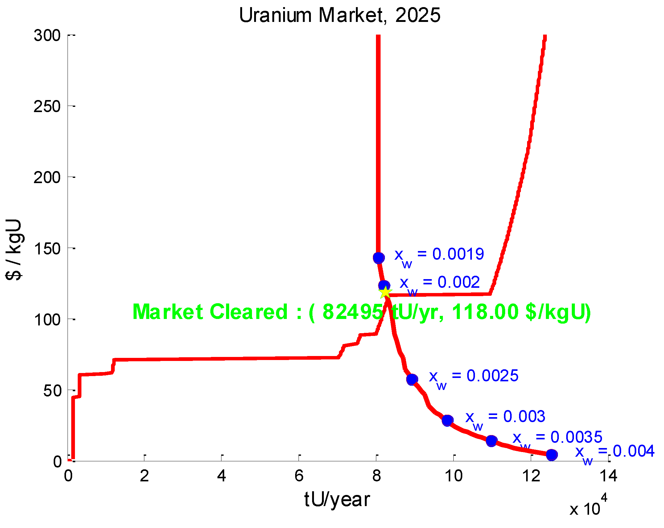
Figure 13 illustrates the supply and demand curves giving rise to the market clearing condition in one arbitrarily selected year, 2025. The xw values noted on the demand curve are the U-235 mass fractions in the enrichment tailings corresponding to the indicated locations on the demand curve. The sloping demand curve illustrates the tradeoff between NU and SWU, as points with lower xw values rely more heavily on enrichment and less heavily on NU purchase to meet enriched uranium fuel demand. The lower the xw value, the more expensive NU would have to be in order to make that tails enrichment optimal. Steps and plateaus in the supply curve, which starts from (0,0) at lower left, indicate the marginal cost of the next unit of NU produced as a function of the NU price. It is important to note that since this model exactly satisfies the enriched U fuel requirements each year, with no option for utilities, enrichers, producers and other market players to build up or draw down inventories or engage in speculation, the model cannot predict spot price excursions such as the one that took place at the end of the decade of the 2000 s. Instead, it is a tool for predicting longer-term price trends, especially in the face of policy decisions or changes in primary or secondary U or SWU supplies.
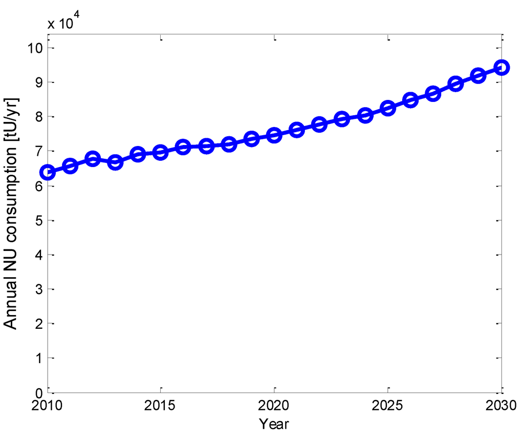
Figure 8.
Annual NU consumption.
Figure 8.
Annual NU consumption.

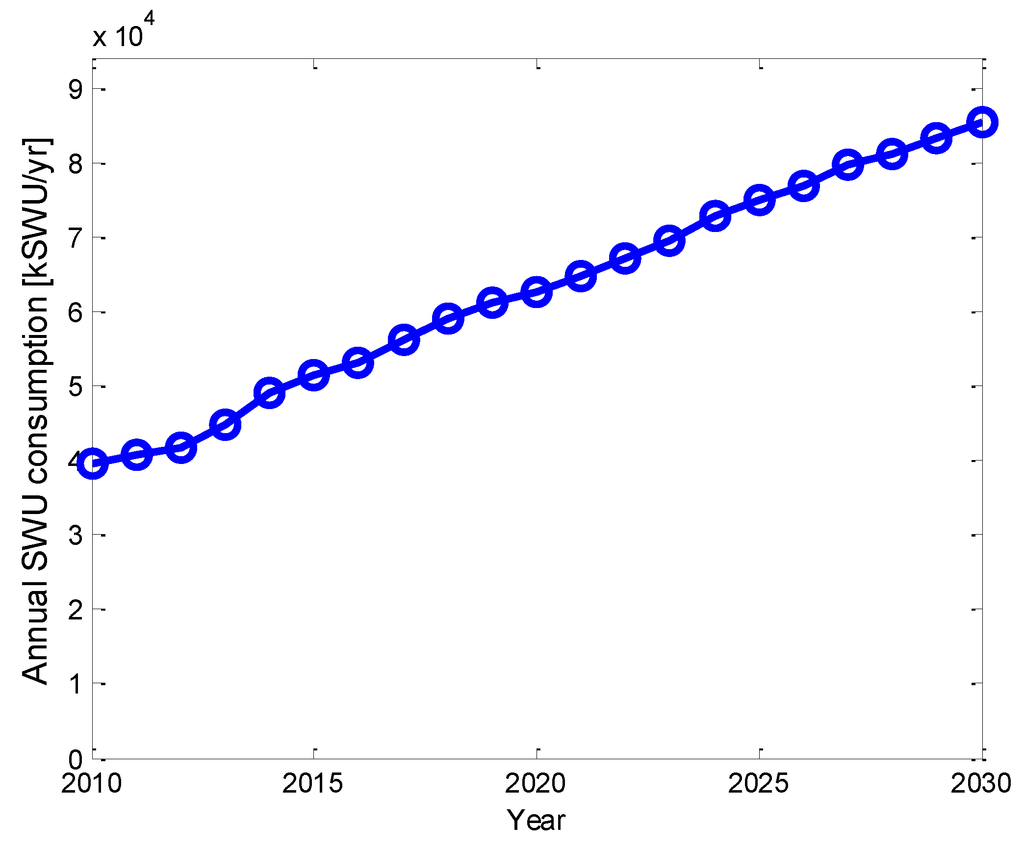
Figure 9.
Annual SWU consumption.
Figure 9.
Annual SWU consumption.
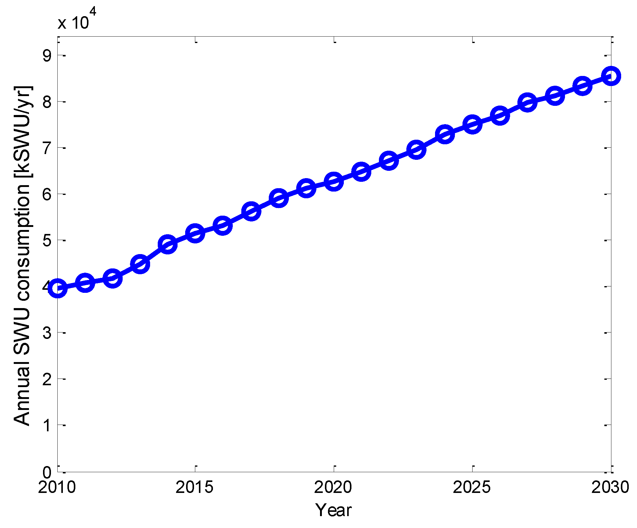

Figure 10.
Market clearing uranium price.
Figure 10.
Market clearing uranium price.
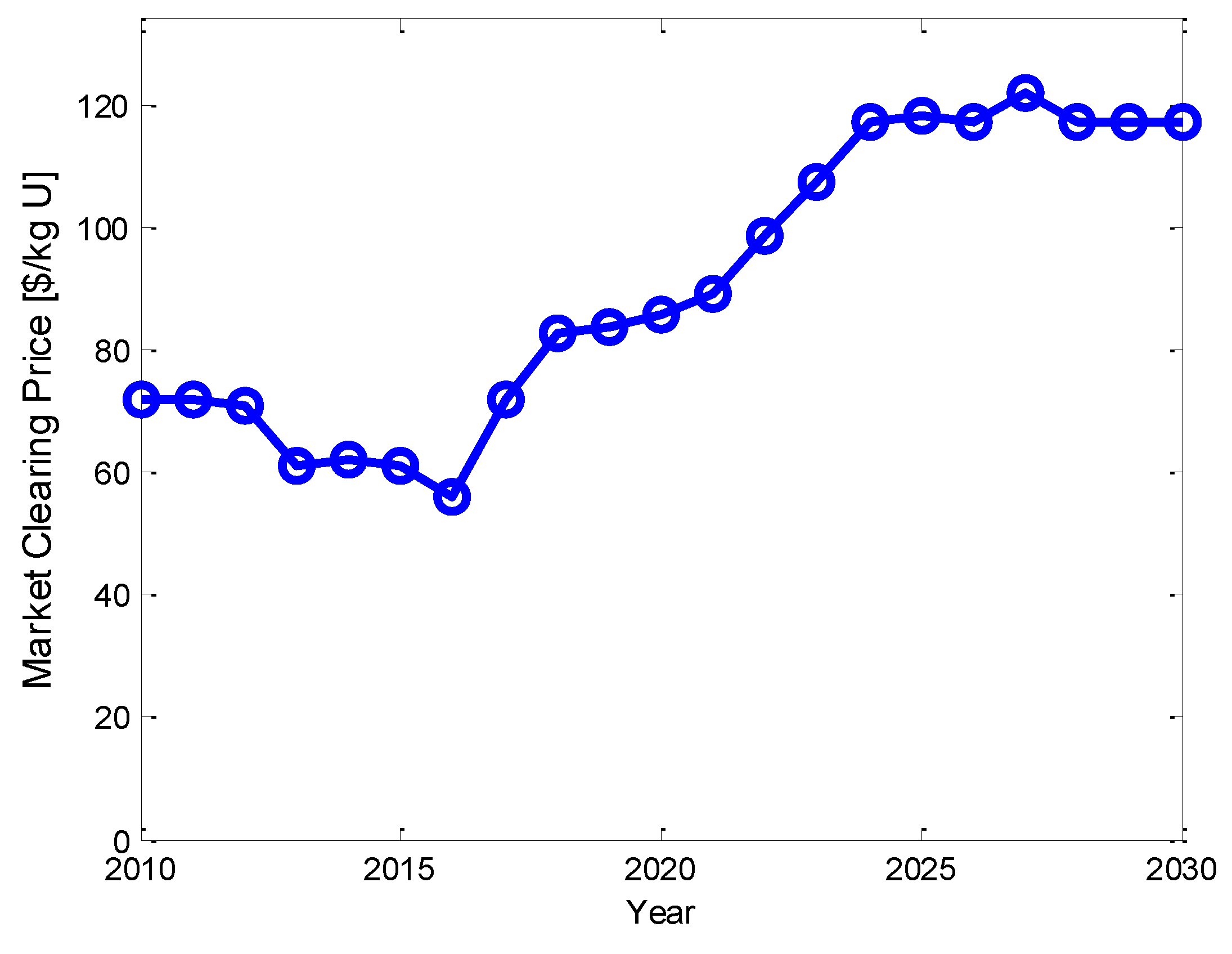
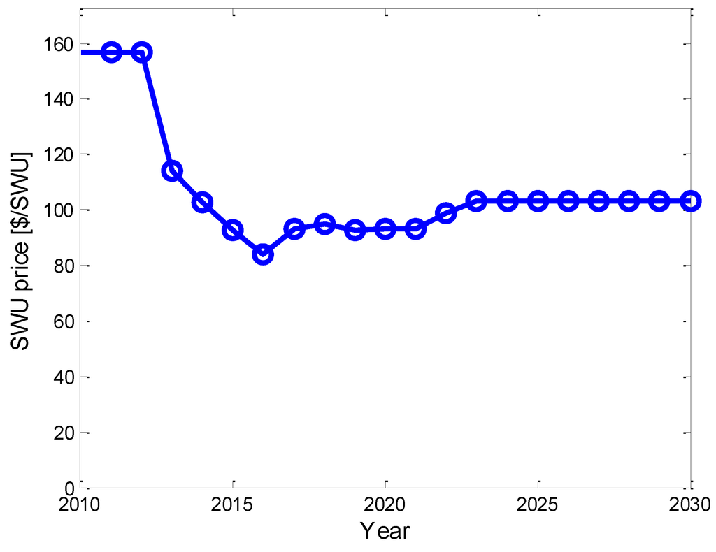
Figure 11.
SWU price.
Figure 11.
SWU price.

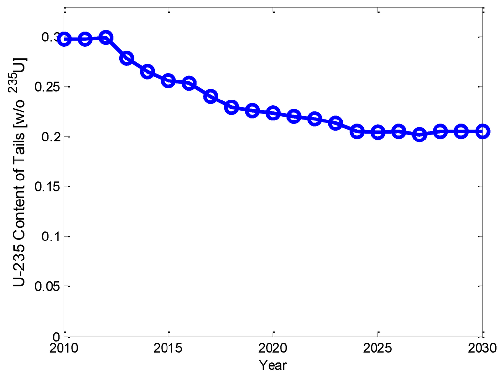
Figure 12.
The tails enrichment.
Figure 12.
The tails enrichment.
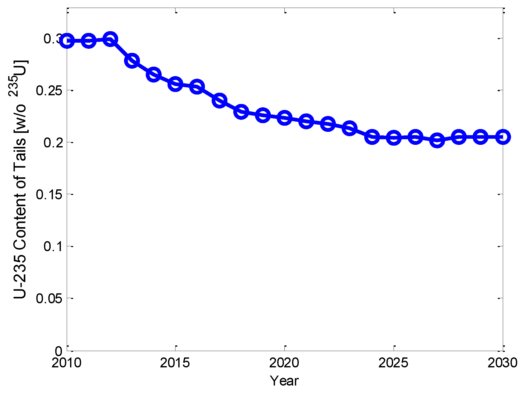

Figure 13.
Uranium market supply and demand curves in 2025.
Figure 13.
Uranium market supply and demand curves in 2025.
4. Conclusions
Using the uranium industry as an example, this paper has presented an approach to modeling the behavior of autonomous entities within a simulation of part of the nuclear fuel cycle. Based upon their unique characteristics, the entities uranium mines made yearly decisions to commence or continue production, or alternatively to enter into short-term or permanent shutdown. The decisions were based upon the economic theory of individual firms with unique supply curves participating in a competitive market. Individual startup and permanent shutdown decisions were myopic in the sense that they took into account only the state of the market in the year they were taken. Therefore, a rollback algorithm was implemented if a mine was found to enter a permanent shutdown condition before it had produced all of its reserves. This algorithm returns the simulation to the year in which the mine was opened and undoes the decision. In that sense, the rollback algorithm replicates firms’ ability to project future market behavior when weighing the costs and benefits of entering an industry.
The work presented here leads to a methodology governing decision-making entities inside a nuclear fuel cycle simulator. A similar algorithm can be envisioned to drive the construction of other fuel cycle facilities as well as power reactors. But it can generalize to entities whose objective is other than maximization of profit. For instance, the decision to construct reactors whose purpose is to burn down transuranic elements may not be driven only by economic considerations. Yet these reactors face a condition similar to the one that led to the rollback algorithm that was demonstrated in this paper for uranium mines. A mine, initially profitable, might later become unprofitable so that its owner would have been better off never having opened it in the first place. Similarly, a transmuter reactor that might have an adequate supply of transuranic fuel at the time it was constructed could face in absence of fuel later on. Within the environment of the fuel cycle simulator, one way to tell whether unfavorable conditions of either type will arise the only way if the simulator is highly complex or nonlinear is to run the simulation clock forward. In both cases, the rollback strategy resolves the unfavorable condition, although it must be noted that this alone does not guarantee that the final outcome of the simulation is in any sense optimal. Nonetheless, the approach represents a step toward autonomous decision making within nuclear energy system models.
Acknowledgments
This publication is based on work supported by Award No. ESP1-7030-TR-11of the U.S. Civilian Research & Development Foundation (CRDF) and by the National Science Foundation under Cooperative Agreement No. OISE-9531011. Specifically, we acknowledge support from the CRDF Global and Estonian Science Foundation 2010 Energy Research Competition (CRDF-ETF II), including award ESP1-7030-TR-11 and ETF award 22/2011. This research was supported by European Social Fund’s Doctoral Studies and Internationalisation Programme DoRa.
Author Contributions
Aris Auzans: Performing analysis and interpretation of data, writing of the manuscript, correspondence with publisher. Erich A. Schneider: Project planning and supervision, including model development, model interpretation and evaluation, and writing of the manuscript. Robert Flanagan: Performing analysis and interpretation of specific data, and writing of the manuscript. Alan H. Tkaczyk: Project planning and supervision, including analysis and evaluation of the model, and writing of the manuscript.
Appendix
Table A1.
Secondary sources.
| Name | Amount (tonnes U or Pu *) | Enrichment (wt% 235U) | Maximum annual rate (tonnes/yr) | Year available | Category |
|---|---|---|---|---|---|
| Purchase Agreement HEU | 100 | 90 | 25 | 2010 | HEU |
| Surplus HEU | 417.1 | 90 | 13.9 | 2014 | HEU |
| Surplus WGPu | 68 | N/A | 3.4 | 2020 | Pu |
| DU-enrichment step A | 291,432 | 0.19 | 14,572 | 2010 | DU |
| DU enrichment step B | 322,804 | 0.24 | 16,140 | 2010 | DU |
| DU enrichment step C | 226,025 | 0.29 | 11,301 | 2010 | DU |
| DU enrichment step D | 254,303 | 0.34 | 12,715 | 2010 | DU |
| DU enrichment step E | 40,147 | 0.39 | 2,007 | 2010 | DU |
| DU enrichment step F | 27,379 | 0.44 | 1,369 | 2010 | DU |
| DU enrichment step G | 1,103 | 0.49 | 55 | 2010 | DU |
| DU enrichment step H | 3,023 | 0.54 | 151 | 2010 | DU |
| DU enrichment step I | 244 | 0.59 | 12 | 2010 | DU |
| DU enrichment step J | 591 | 0.64 | 30 | 2010 | DU |
* Plutonium.
Table A2.
Global input parameters.
| Description | Mean Value |
|---|---|
| World LEU fuel demand in 2010 | 6790 tonnes/yr |
| World NU fuel demand in 2010 * | 3390 tonnes/yr |
| Average 235U content of LEU fuel | 4.3 wt% |
| World LEU & NU fuel demand growth rate | 2.6%/yr |
| Year continuous enrichment facility capacity growth commences | 2018 |
| Enrichment facility capacity growth rate | 2.6%/yr |
| Cost of yellowcake-to-fluoride conversion | $10/kg U |
| WGPu fraction in MOX ** | 5 wt% of IHM |
| 235U content of HEU downblend stock | 0.25 wt% |
| Uranium Production Cost Multiplier | 1.0 |
| SWU Production Cost Multiplier | 1.0 |
| Mine Capacity Factor Multiplier | 1.0 |
* Certain reactors, e.g., CANDU, consume fuel fabricated from unenriched natural uranium. ** Mixed oxide fuel.
Table A3.
LEU demand.
| Enrichment supply growth * | 2010 | 2011 | 2012 | 2013 | 2014 | 2015 | 2016 | 2017 | 2018 | 2019 | 2020 and beyond | Type | SWU Cost |
|---|---|---|---|---|---|---|---|---|---|---|---|---|---|
| Name | kSWU/yr | kSWU/yr | kSWU/yr | kSWU/yr | kSWU/yr | kSWU/yr | kSWU/yr | kSWU/yr | kSWU/yr | kSWU/yr | kSWU/yr | $/SWU | |
| USEC ACP | 0 | 0 | 0 | 0 | 1,000 | 2,400 | 3,800 | 3,800 | 3,800 | 3,800 | 3,800 | C | 103 |
| URENCO NEF | 1,180 | 2,360 | 3,540 | 4,720 | 5,900 | 5,900 | 5,900 | 5,900 | 5,900 | 5,900 | 5,900 | C | 63 |
| Areva Eagle Rock | 0 | 0 | 0 | 0 | 1,100 | 1,100 | 2,200 | 2,200 | 3,300 | 3,300 | 3,300 | C | 75 |
| Eurodif Besse II | 0 | 1,250 | 2,500 | 3,750 | 5,000 | 6,250 | 7,500 | 7,500 | 7,500 | 7,500 | 7,500 | C | 62 |
| Brazil Resende | 0 | 0 | 0 | 0 | 0 | 120 | 120 | 120 | 120 | 120 | 120 | C | 160 |
| Urenco Capenhurst | 5,000 | 5,000 | 5,000 | 5,000 | 5,000 | 5,000 | 5,000 | 5,000 | 5,000 | 5,000 | 5,000 | C | 70 |
| Urenco Almelo | 3,800 | 4,150 | 4,150 | 4,500 | 4,500 | 4,500 | 4,500 | 4,500 | 4,500 | 4,500 | 4,500 | C | 73 |
| Urenco Gronau | 2,200 | 2,200 | 2,200 | 2,775 | 3,350 | 3,925 | 4,500 | 4,500 | 4,500 | 4,500 | 4,500 | C | 84 |
| JNFL Rokkasho | 150 | 150 | 300 | 450 | 600 | 750 | 900 | 1,050 | 1,200 | 1,350 | 1,500 | C | 93 |
| Tenex UEKhK | 9,800 | 9,800 | 9,800 | 9,800 | 9,800 | 9,800 | 9,800 | 9,800 | 9,800 | 9,800 | 9,800 | C | 35 |
| Tenex EKhZ | 5,800 | 5,800 | 5,800 | 5,800 | 5,800 | 5,800 | 5,800 | 5,800 | 5,800 | 5,800 | 5,800 | C | 40 |
| Tenex SKhK | 2,800 | 2,800 | 2,800 | 2,800 | 2,800 | 2,800 | 2,800 | 2,800 | 2,800 | 2,800 | 2,800 | C | 48 |
| Tenex Angarsk | 2,600 | 3,600 | 3,600 | 4,600 | 4,600 | 5,600 | 5,600 | 6,600 | 6,600 | 7,600 | 7,600 | C | 53 |
| USEC Paducah | 8,000 | 8,000 | 4,000 | 0 | 0 | 0 | 0 | 0 | 0 | 0 | 0 | D | 163 |
| Eurodif Georges Besse | 11,300 | 9,417 | 7,534 | 5,651 | 3,768 | 1,885 | 0 | 0 | 0 | 0 | 0 | D | 157 |
| CNNC Heping | 400 | 400 | 400 | 400 | 400 | 400 | 400 | 400 | 400 | 400 | 400 | D | 129 |
| CNNC Hanzhong | 500 | 500 | 500 | 500 | 500 | 500 | 500 | 500 | 500 | 500 | 500 | C | 107 |
| CNNC Lanzhou | 500 | 500 | 500 | 500 | 500 | 500 | 1,000 | 1,000 | 1,000 | 1,000 | 1,000 | C | 89 |
* There are no announced capacity additions after 2020. See Section II.B in [2] for discussion of enrichment supply growth assumption under conditions of substantial LEU demand growth.
Conflicts of Interest
The authors declare no conflict of interest.
References
- 2013 Uranium Marketing Annual Report; U.S. Department of Energy: Washington, DC, USA, 2014.
- The Global Nuclear Fuel Market: Supply and Demand 2011–2030; World Nuclear Association: London, UK, 2008.
- Nuclear Energy Data; OECD Technical Report NEA-6893; OECD Nuclear Energy Agency: Paris, France, 2010.
- Schneider, E.A.; Phathanapirom, U.; Eggert, B.R.; Segal, E. A market-clearing model of the uranium and enrichment industries. Nucl. Technol. 2013, 183, 160–177. [Google Scholar]
- Eggert, R.; Gilmore, A.; Segal, E. Expanding Primary Uranium Production: A Medium-Term Assessment,” Colorado School of Mines Report; Colorado School of Mines: Golden, CO, USA, 2011. [Google Scholar]
- Licensing Process for New Uranium Mines and Mills in Canada; Minister of Public Works and Government Services Canada Catalogue Number CC172-40/2007E-PDF; Canadian Nuclear Safety Commission: Ottawa, ON, Canada, 2007.
- Nechyba, T.J. Microeconomics, an Intuitive Approach with Calculus; South-Western Cengage Learning: Mason, OH, USA, 2011. [Google Scholar]
- Diehl, P. WISE Uranium Project. Available online: http://www.wise-uranium.org/ (accessed on 29 July 2011).
- Economic Modeling Working Group (EMWG) of the Generation IV International Forum. Cost Estimating Guidelines for Generation IV Nuclear Energy Systems; OECD Nuclear Energy Agency: Paris, France, 2007. [Google Scholar]
- Harshbarger, R.J.; Reynolds, J.J. Mathematical Applications for the Management, Life, and Social Sciences, 9th ed.; Cengage Learning: Boston, MA, USA, 2009. [Google Scholar]
© 2014 by the authors; licensee MDPI, Basel, Switzerland. This article is an open access article distributed under the terms and conditions of the Creative Commons Attribution license (http://creativecommons.org/licenses/by/4.0/).