4.1. Results from CFD Analysis
There are several methods to predict the aerodynamic characteristics of wind turbines [
21,
22]. In this study, the full 3D CFD approach with the rotating blade was adopted using the commercial CFD software, ANSYS-CFX.
Figure 6 shows the C
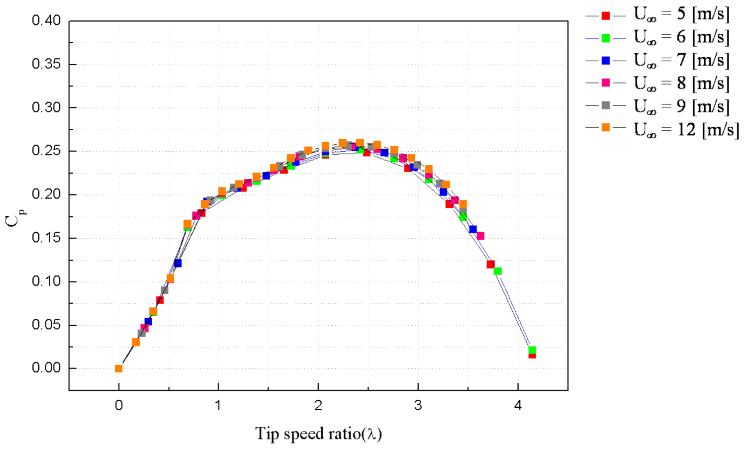
p versus tip speed ratio curve obtained by the CFD analysis when the velocity was changed from 5 to 12 m/s for the 0.5 kW Archimedes wind turbine. The in-flow wind profile was assumed to be uniform. The maximum power coefficient observed near a tip speed ratio of approximately 2.5 was approximately 0.25. The power coefficient curves showed a similar tendency regardless of the velocities. The modern urban-usage 3-blade and Darrieus blade type wind turbines have high rotor efficiency up to 0.25 in the high tip speed ratio range [
8,
10]. This means that high efficiency can be achieved in the case of a high wind speed. On the other hand, in an urban environment, the wind velocities are usually less than 3 m/s [
8]. However, the local wind speed can vary substantially depending on the location, for example it may be much higher above the roof of a large building. The spiral wind blade with an Archimedes shape shows relatively high rotor efficiency compared to the aerodynamic performance of the other blades like the Savonius type rotor in the lower tip speed ratio range [
23]. In addition, the Archimedes spiral blade had high C
p values over a wider range of tip speed ratios.
Figure 6.
Cp-Tip speed ratio with respect to the wind velocity.
Figure 6.
Cp-Tip speed ratio with respect to the wind velocity.
Figure 7 shows torque according to the rotating speed for a comparison of the theoretical prediction with the numerical results. In the case of the theoretical result, the torque for the rotating speed has a gradual decreasing tendency at U = 5 m/s. The results of the torque for wind power generation through numerical analysis showed a similar tendency to the theoretical analysis. From this result, the numerical analysis appears to show relatively good agreement at the operating rotational speed regions.
Figure 7.
Comparison of the theoretical prediction with the numerical results (U = 5 m/s).
Figure 7.
Comparison of the theoretical prediction with the numerical results (U = 5 m/s).
A comparative study of the CFD and PIV experiment was performed to validate the CFD results to be used as a design tool for the Archimedes wind turbine. For this purpose, the geometry of the wind turbine blade, the inlet velocity profile and rotating speeds of the blade for CFD analysis were the same as the experimental conditions.
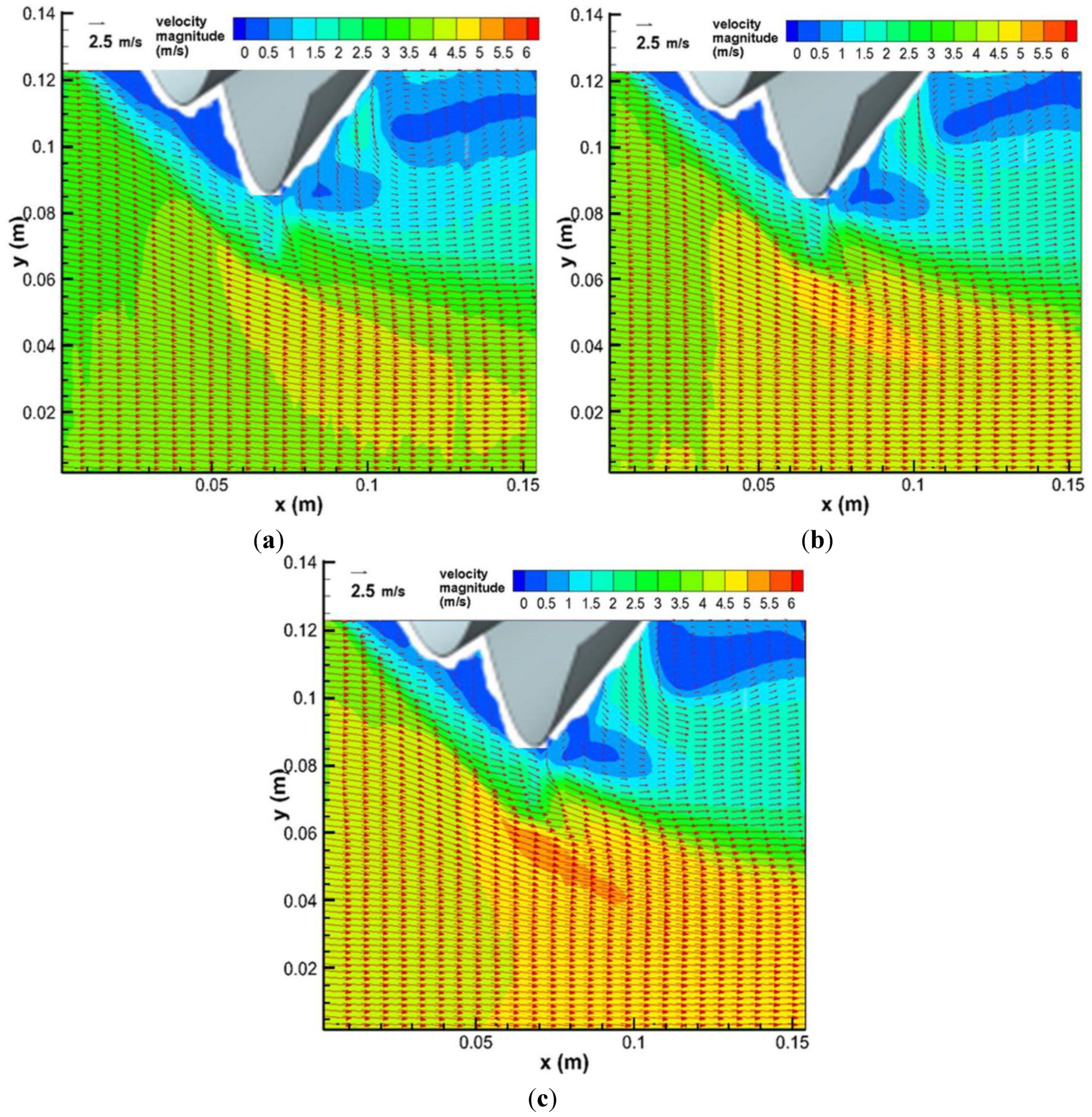
Figure 8 shows the calculated ensemble averaged velocity fields of the overall flow field on the central plane of the Archimedes spiral wind turbine at three different wind speeds, which were characterized by the contours and velocity vectors. The rotating velocities measured at in-flow velocities of 3.5, 4.0 and 5.0 m/s were 300, 400 and 500 rpm, respectively. The corresponding tip speed ratios were 0.62, 0.78 and 0.79, respectively. Remarkably, details of the flow behavior were obtained over a range of wind velocities. Indeed, the contours shown in these figures correspond to the turbulent wake shape.
Figure 8.
Ensemble-averaged velocity fields obtained by the steady simulation: (a) 3.5 m/s and 300 rpm; (b) 4 m/s and 400 rpm; (c) 5 m/s and 500 rpm.
Figure 8.
Ensemble-averaged velocity fields obtained by the steady simulation: (a) 3.5 m/s and 300 rpm; (b) 4 m/s and 400 rpm; (c) 5 m/s and 500 rpm.
The highest velocities were observed in the vicinity of the rotor tip in the calculation domain. Because of the spiral effect, the velocities from the leading edge increased at the inner side of each blade. A recirculation zone with lower speeds was also observed in the wake regions because the incoming airflow was blocked by the hub cone and rotor. A circular accelerating zone existed behind the rotor, which resulted in a low pressure near the wall of the rotating domain. A low-speed region formed behind the hub of the rotor, indicating the wake region. The size of the recirculating zone was approximately one and half diameters long from the back side of the rotor and the maximum width of the wake region was equal to the rotor diameter.
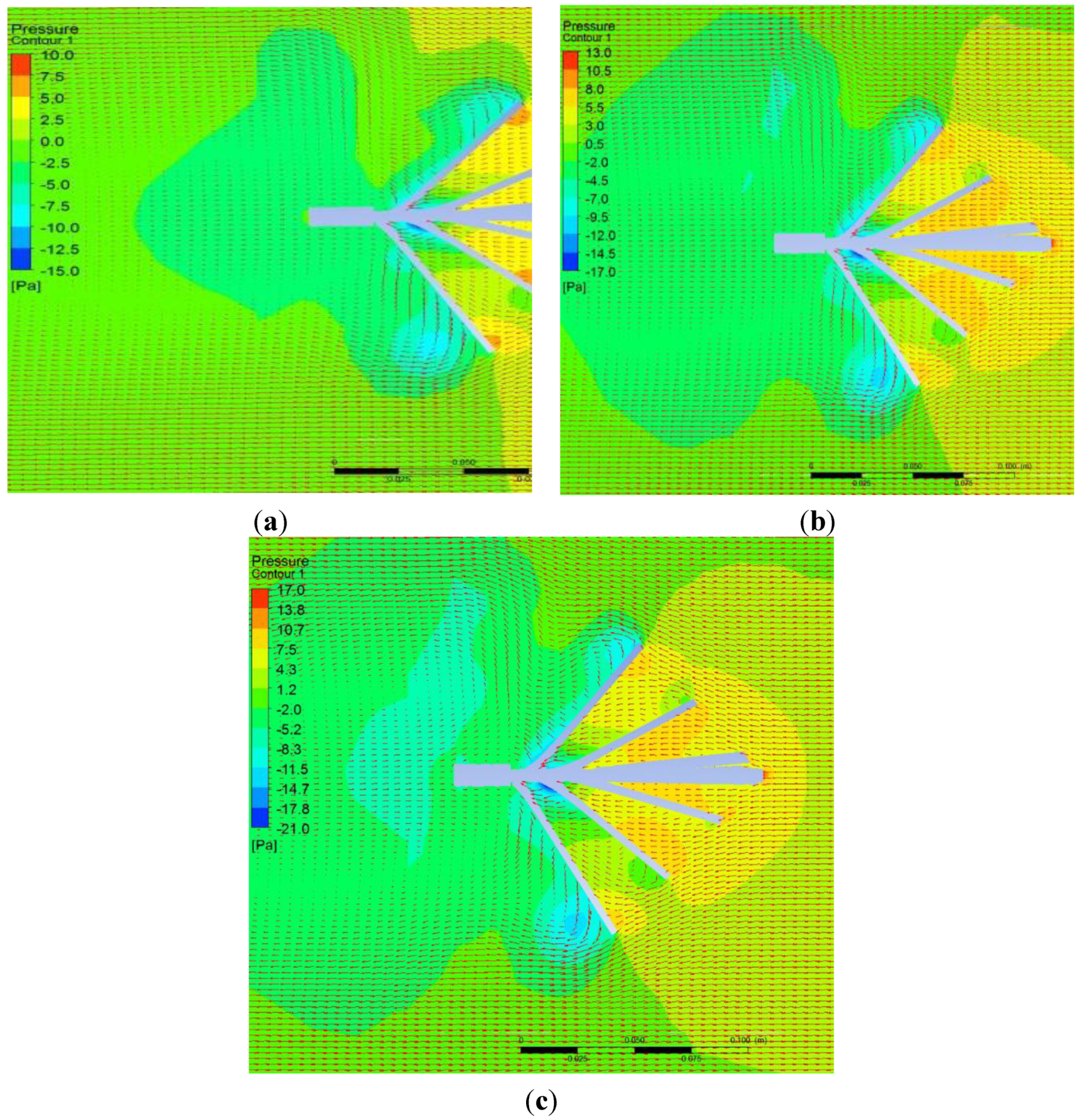
Figure 9 shows the pressure distribution in the center plane of the wind turbine. The flow direction was from right to left. When the blade is rotating, there is a pressure difference between the pressure side and the suction side. Due to the spiral surface of the blades, the pressure difference (a force) generates torque. In general, the front side of the blade has higher pressure while the corresponding rear side has a lower pressure.
Figure 9.
Static pressure distribution obtained by the steady simulation (a) 3.5 m/s and 300 rpm; (b) 4 m/s and 400 rpm; (c) 5 m/s and 500 rpm.
Figure 9.
Static pressure distribution obtained by the steady simulation (a) 3.5 m/s and 300 rpm; (b) 4 m/s and 400 rpm; (c) 5 m/s and 500 rpm.
When the in-flow velocity increases, the pressure difference becomes larger. The pressure difference is large at the blade tip but small at the root region. This means that most of energy can be extracted near the blade tip like a three blade HAWT. The pressure differences between the root and tip were approximately 3 Pa. On the suction side, however, the pressure differences were much higher. The pressure differences were more than 15 Pa (even more than 20 Pa at wind speeds of 4 and 5 m/s) lower at the tip than the root. Therefore, the pressure difference between the two sides at a section increase towards the tips of each blade. For the three cases, the rear side pressure is negative, so that thrust force can be exerted to the shaft.
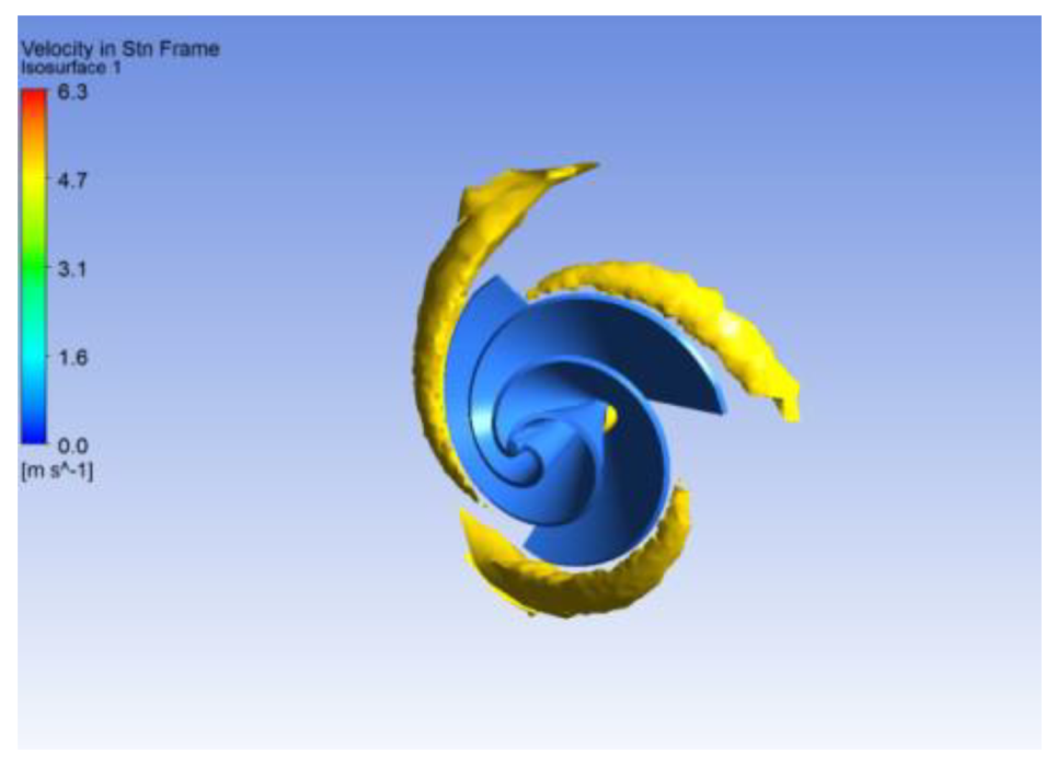
Figure 10 shows the vortical structures represented by the isosurface of the swirl strength in case of different wind speeds. The swirl strength was calculated based on a three-dimensional unsteady simulation. The maximum swirl strength occurred in the tip vortex. A threshold swirl strength, which is 50% of the maximum strength, was selected and the vortical structures were rendered using iso-surface of the swirl strength. The near wake structure of the Archimedes spiral wind turbine was different from the structure of tip vortex generated by the general HAWT type wind turbine. Owing to the spiral shape of the blade, the evolution of the tip vortex developed in a spiral manner, and the core of the tip vortex was removed from the edge of the blade along the downstream direction. The swirl strength became stronger with increasing wind speed.
Figure 10.
Vortical structures represented by the isosurface of the swirl strength (unsteady simulation, 5.0 m/s, and 500 rpm).
Figure 10.
Vortical structures represented by the isosurface of the swirl strength (unsteady simulation, 5.0 m/s, and 500 rpm).
4.2. Experimental Results
Three speeds were measured at the exit of the open circuit wind tunnel, which are uniform in-flow velocities to the experimental model. Based on the diameter of the blade and uniform flow velocities, 3.5, 4.0 and 5.0 m/s, the Reynolds numbers were 34,770, 39,740 and 49,670, respectively.
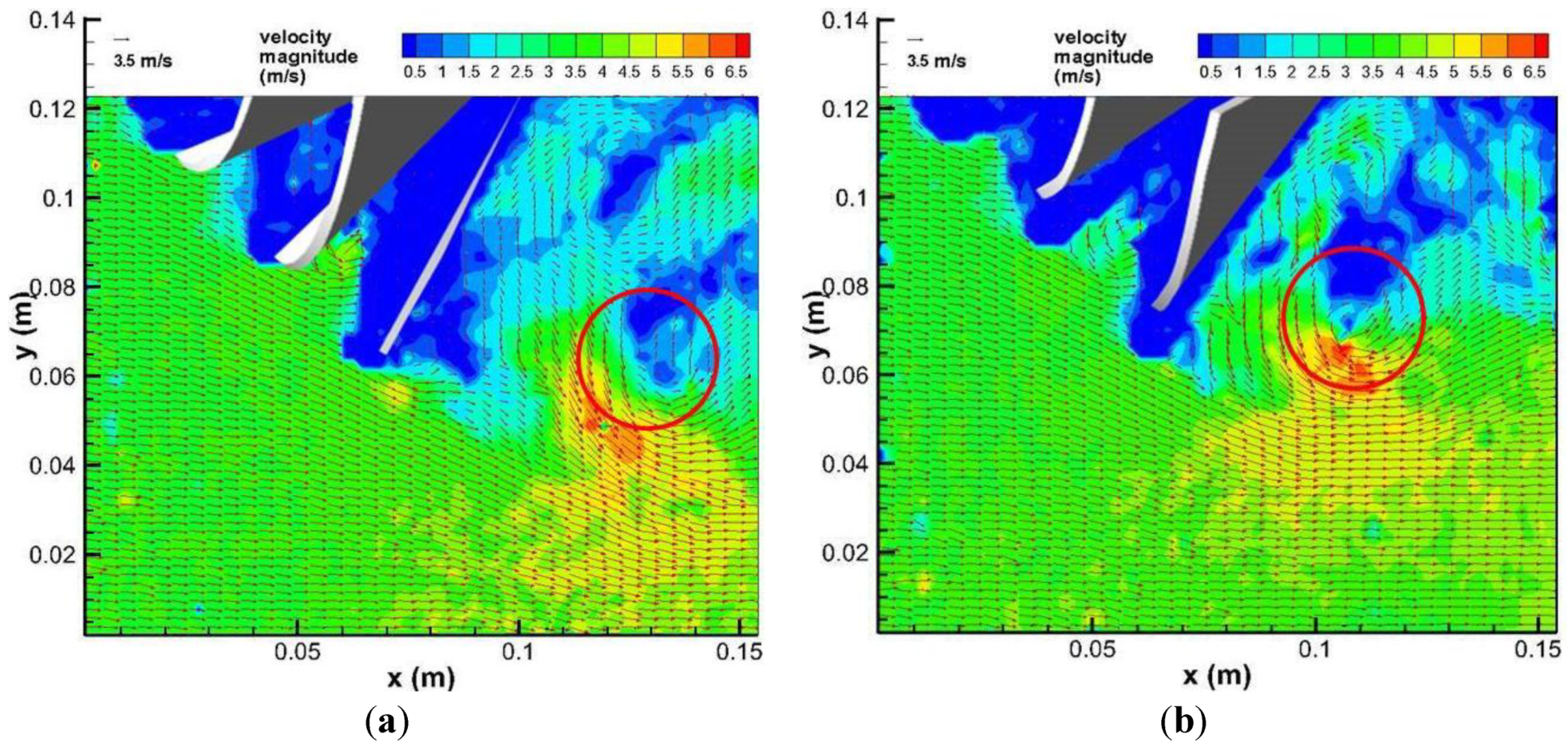
Figure 11 shows the mean velocity contour obtained at a 0° angle of attack. Owing to the presence of the Archimedes spiral blade, the decrease in mean velocity was observed while the incoming airflow passes through the surface of the blades. The streamwise momentum was converted to the angular momentum because of the rotation of the blade followed by a decrease in the mean velocity in this region. After passing through the blade, the air velocity was also decreasing. On the other hand, there was no flow separation because the flow passage through the blade was increasing. According to the momentum conservation law, the momentum deficit which is induced by the decreasing streamwise velocity after the wind turbine can be transformed to the power of the blade shaft. The maximum velocity region was located at the position of the maximum diameter of the blade, approximately one radius outside.
The low speed region was attributed to the tip vortex region. Free stream flow was observed outside of the tip vortex region, and there was a strong shear layer in the edge of the near wake. Turbulence generation would be great in this region because of the high shear rate and large turbulent shear stress. A low velocity region was observed near the shaft approximately one diameter of the blade downstream. This suggests that this region is caused by swirling motion of the near wake.
Figure 11.
Ensemble averaged velocity fields obtained by the PIV measurements. (a) 3.5 m/s and 300 rpm; (b) 4 m/s and 400 rpm; (c) 5 m/s and 500 rpm.
Figure 11.
Ensemble averaged velocity fields obtained by the PIV measurements. (a) 3.5 m/s and 300 rpm; (b) 4 m/s and 400 rpm; (c) 5 m/s and 500 rpm.
Figure 12 presents the turbulent kinetic energy (TKE) distribution in the tip vortex of the wind turbine. As the out of plane component (w’) of velocity fluctuation was not measured, the TKE was obtained using 1/2(u’
2 + 2 v’
2) assuming that w’ is equal to v’. The turbulent kinetic energy can be generated by random fluctuations and periodical oscillations of unsteady flow. The TKE levels along the tip vortex structures were quite high with the highest TKE level being observed in the wake of the wind turbine model. The high TKE levels in this area are related to the generation of tip vorticity and flow separation around the wind turbine blade, as shown clearly from the ensemble averaged PIV measurement results.
Figure 12.
Turbulent kinetic energy distribution (a) 3.5 m/s and 300 rpm; (b) 4 m/s and 400 rpm; (c) 5 m/s and 500 rpm.
Figure 12.
Turbulent kinetic energy distribution (a) 3.5 m/s and 300 rpm; (b) 4 m/s and 400 rpm; (c) 5 m/s and 500 rpm.
The aerodynamic characteristics in the near wake of the blades, particularly the tip vortex flow structure, were examined by measuring the instantaneous velocity fields at different phase angles using a PIV experiment. The aerodynamic characteristics at the different relative positions of the Archimedes spiral wind turbine blades can be determined from the contours of the instantaneous velocity and vorticity fields for the different phases during the more comprehensive processing of blade rotation. In general, the aerodynamic characteristics of the instantaneous fields can be reflected more accurately by identifying more phase angles. The range of phase angles is often decided by the number of blades because one cycle of the rotating blades is 360°. Most HAWTs, which include the Archimedes spiral wind turbine, have three centrosymmetrical blades [
20]. This means that there are three repeated processes during a single cycle. For one process of the blade of a wind turbine, the range of phase angles is 120°. Accordingly, the range of phase angles from 0° to 120° was selected because of the three centrosymmetrical blade structure of the Archimedes spiral wind turbine.
A mini-Nd:Yag laser (150 mJ/pulse) was used to obtain a particle image at 15 frames per second. The PIV system was synchronized using the rotational speed meter. To obtain the phase-averaged velocity field, the PIV realizations matching with the phase angles were selected. During the experiment, the blade location and laser firing sequences were recorded. The instantaneous PIV measurement results with an incoming airflow velocity of 3.5 m/s and a wind turbine blade rotation speed of 300 rpm were analyzed to determine the instantaneous images of the wake vortex structures at different phase angles, as shown in
Figure 13. At the same time, the phase angle was changed from 0° to 120° at 20° intervals. It is difficult to resolve the evolution of tip vortex structure by the standard two-dimensional PIV realizations, however the signature of the tip vortex can be recognized clearly near the outermost blade of the Archimedes spiral wind turbine with respect to the change in phase angle as marked red circles in
Figure 13. At a phase angle of α = 0°, the outermost wind turbine blade was in the most downward position. When the phase angle was increased, the outermost wind turbine blade rotated out of the vertical PIV measurement plane. The second wind turbine blade would rotate out into the PIV measurement plane at a phase angle of α = 120°. This shows that as the phase angle is increased, the displacements of the tip vortex structures are transmitted downstream. In contrast to the conventional horizontal wind turbine, the velocity at the core area of the tip vortex induced from the spiral wind turbine is higher due to the spiral-shaped blades, which can increase the airflow speed through the spiral-shaped surface. An examination of the inner blade to the outer layer showed that the movement of the tip vortex coincided approximately with the blade gradual direction. The trajectory of the trailing vortex coincides with the strong shear layer region in the mean velocity field. For all cases of different phase angles, there were no interactions between the tip vortices generated from the three blades.
Figure 13.
Instantaneous velocity field of the PIV measurements (Tip phase change) (a) α = 0°; (b) α = 40°; (c) α = 80°; (d) α = 120°.
Figure 13.
Instantaneous velocity field of the PIV measurements (Tip phase change) (a) α = 0°; (b) α = 40°; (c) α = 80°; (d) α = 120°.
4.3. Comparison of the PIV Measurement and CFD Simulations
Figure 14 presents the PIV and CFD results at 300 rpm and a 3.5 m/s wind velocity. To compare the results of the CFD simulation and PIV experiment, the line data of the ensemble-averaged velocity fields were selected as indicated in
Figure 14a. The wind velocity of the experiment was higher than that in CFD, and initially, there was a downward tendency that reflected the situation from upstream to downstream through the core of the tip vortex structure. An assessment of those responses on the ensemble averaged velocity field of the PIV measurements showed that as the relative incoming airflow decreases, the tip vortex structures and wake velocity can be influenced more easily because of the spiral-shaped blade. In the lower tip-speed-ratio case, the affected region was wider than that of under higher conditions. The results of the PIV and unsteady CFD showed a similar trend distribution, as shown in
Figure 14. The flow was mainly attached and only separated at the core of the tip vortex. This means that the downstream mean velocity in the core of the tip vortex of the PIV is lower than that in the CFD simulation. The boundary sections of the PIV or unsteady state CFD were similar. A comparison of the ensemble-averaged velocity field and the pressure field showed that the flow could not attach on the blade any longer, and the boundary layer separated, resulting in a separated vortex form. This is because the low pressure area of the suction side moved gradually to the blade tip edge when the dynamic pressure was less than the adverse static pressure. Subsequently, the main separated vortex increased further and the region affected was even larger. A comparison of the PIV measurement with the CFD numerical simulation showed that the vector diagram almost agreed with each other, particularly in the shape and vector trend, as well as the position and size of the tip vortex.
Figure 14.
Comparison of the PIV experimental and CFD (steady and unsteady state) results (300 rpm and U∞ = 3.5 m/s). (a) Line Data Extracting Location for the Velocity Profile; (b) Velocity Profile at Line 1; (c) Velocity Profile at Line 2; (d) Velocity Profile at Line 3; (e) Velocity Profile at Line 4.
In the unsteady state simulation, when the air flow passed the blade, the flow needed to accelerate to pass the blade surface. As the air continuously passed the wind turbine blade, it created a low-pressure area on the tip of the blade because the wind across this area had a higher velocity. On the other hand, the steady state cases were different from the unsteady state because the steady state simulation did not change the relative position between the blade and incoming airflow. In the steady state simulation, the multiple reference frames (MRF) technique was used. The URANS is able to resolve some important structures that occur due to unsteady effects in the rotation, which RANS cannot resolve due to the averaging.

 ,
, 


