
Thermal Model of a Dish Stirling Cavity-Receiver


Abstract
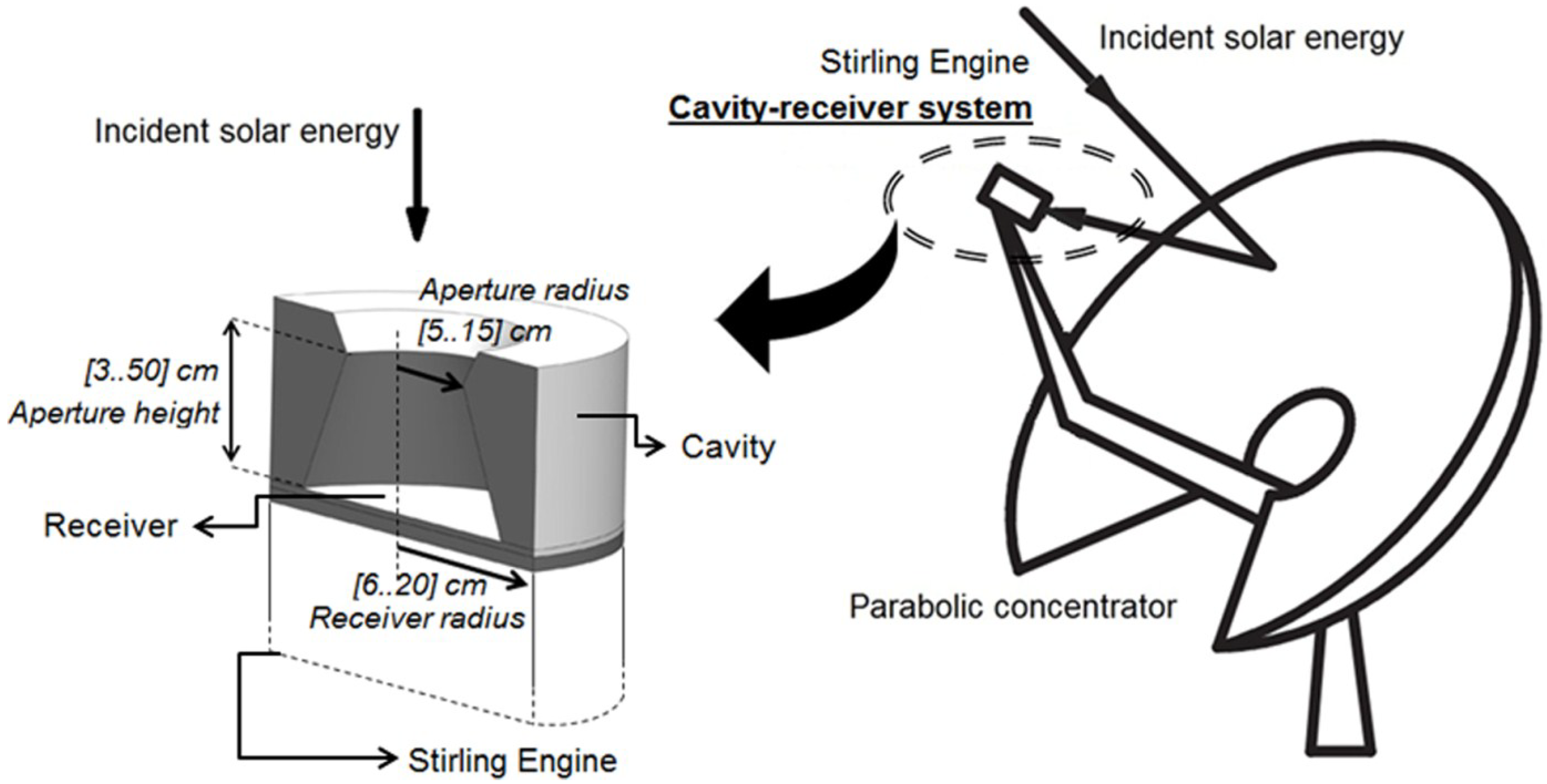
:1. Introduction
2. Methodology

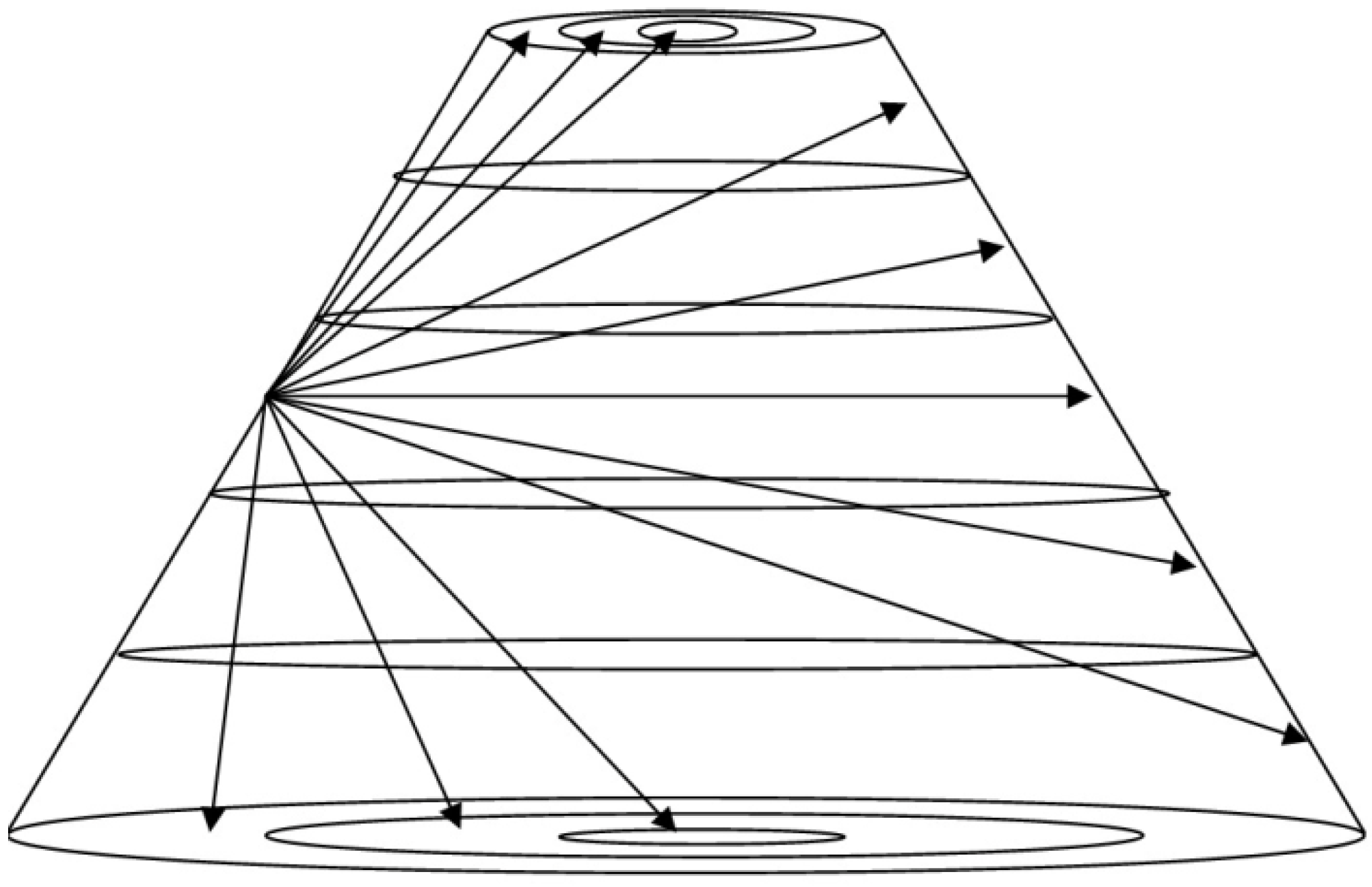
2.1. Radiation Exchange


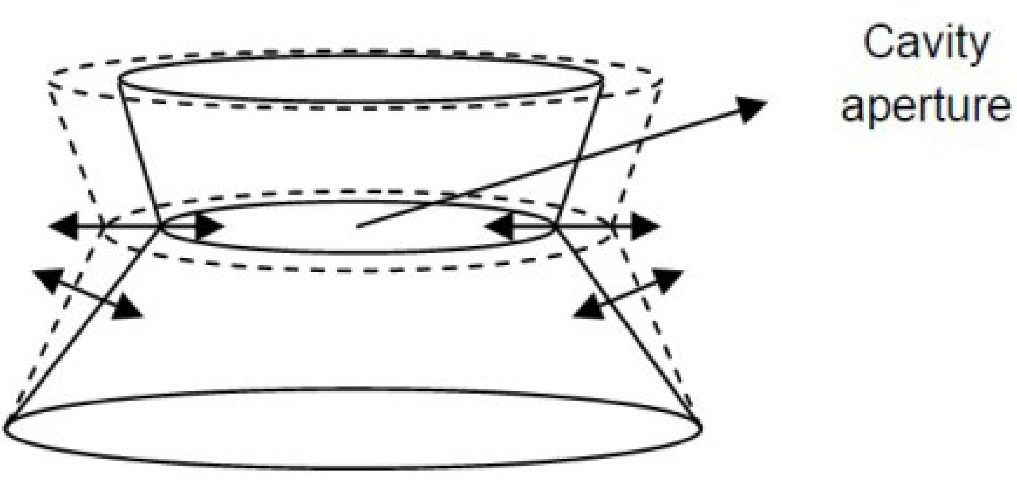
2.2. View Factors
- -
- Sum law:
- -
- Reciprocity law:
- -

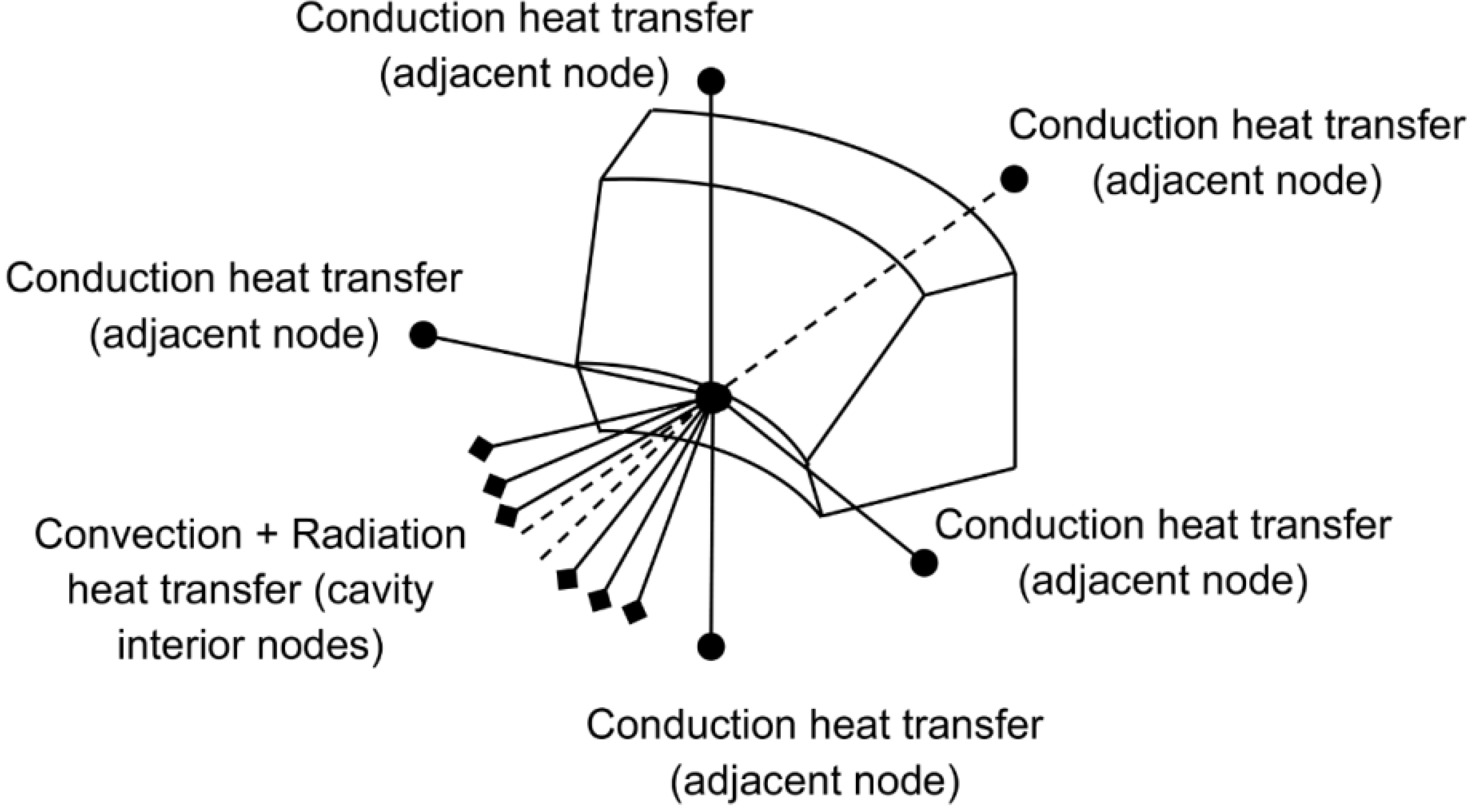
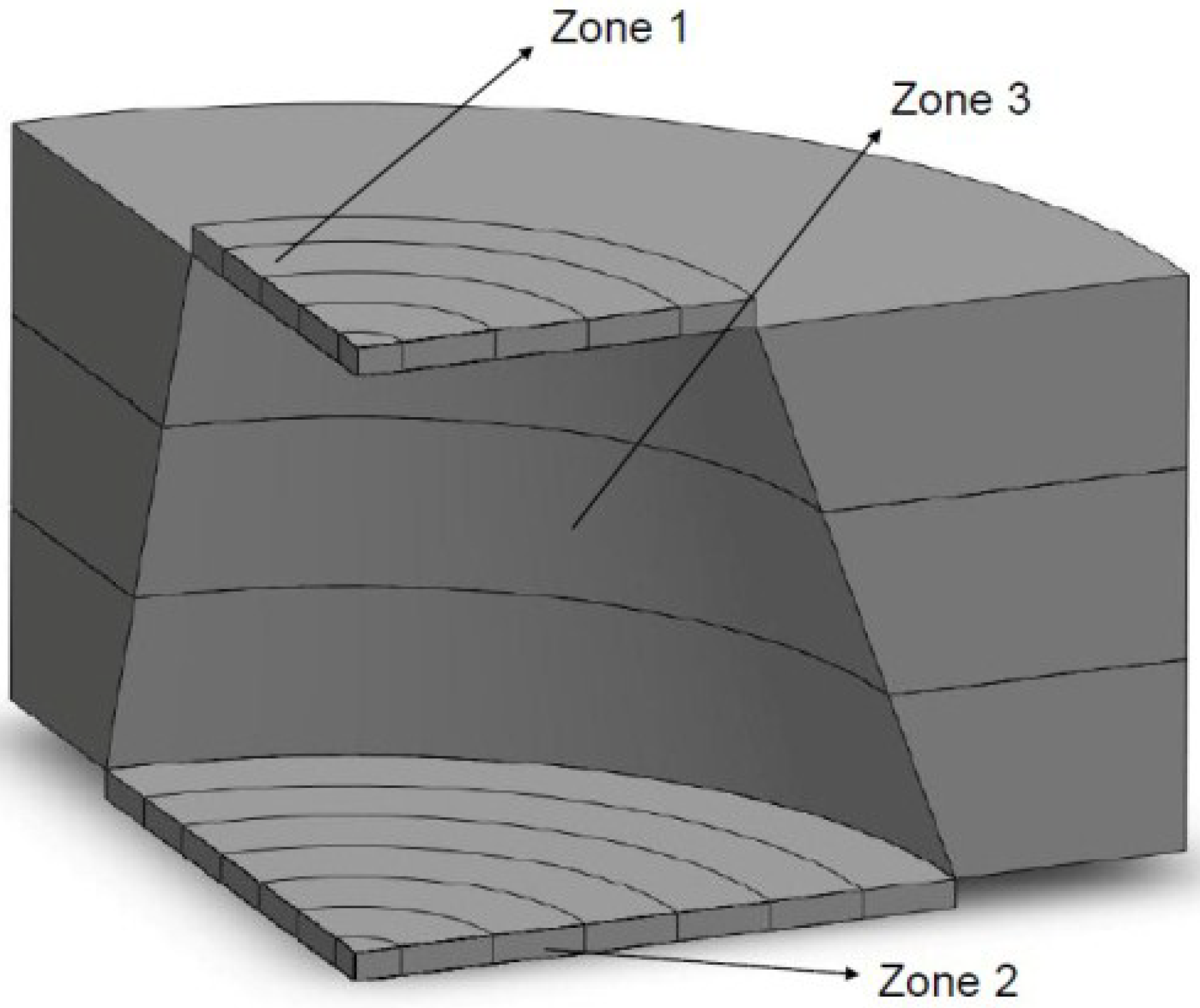
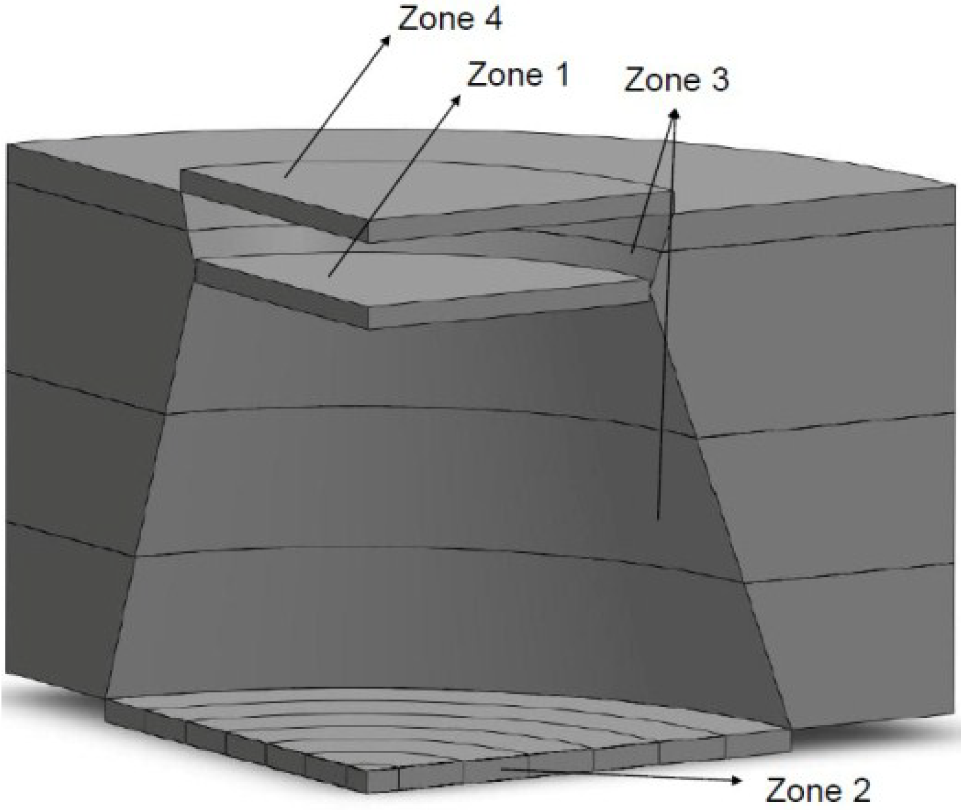
2.3. Finite Differences
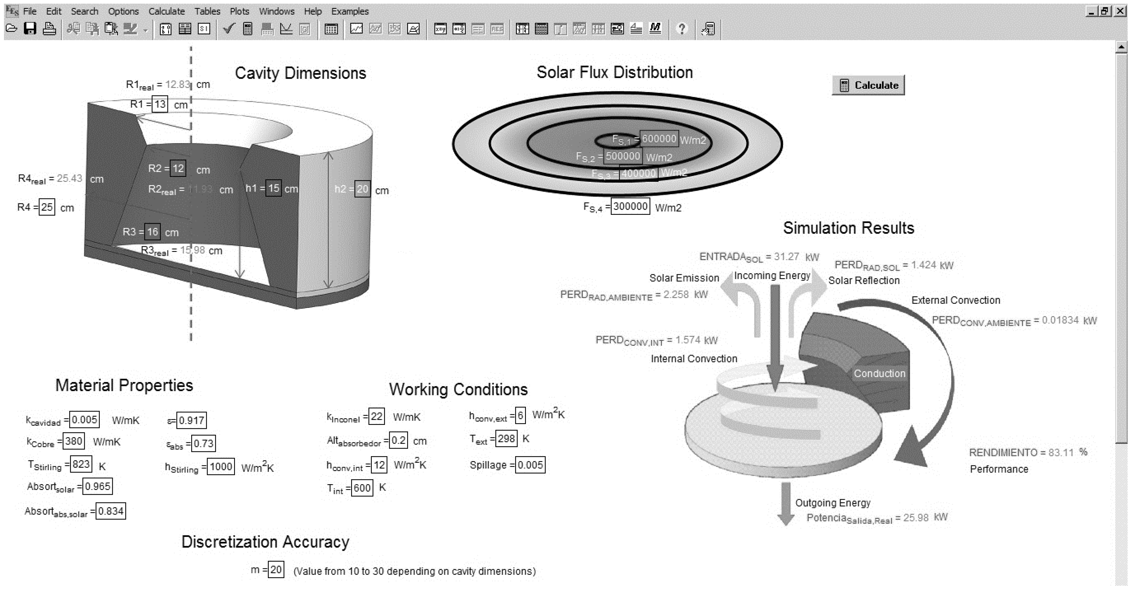
3. Cavity Optimization with the EES tool


| Material Properties | |
| Cavity Absorptivity [-] | 0.965 |
| Absorber Absorptivity [-] | 0.834 |
| Cavity Emissivity [-] | 0.917 |
| Absorber Emissivity [-] | 0.73 |
| Cavity Conductivity [W/mK] | 0.005 |
| Equivalent Convection Coefficient [W/m2K] | 6 |
| Equivalent Interior Air Temperature [K] | 600 |
| Environment Temperature [K] | 298 |
| Geometrical Parameters | |
| Reconcentrator Radius [cm] | 13.28 |
| Aperture Radius [cm] | 10.13 |
| Receiver Radius [cm] | 15.98 |
| External Cavity Radius [cm] | 25.43 |
| Aperture Height [cm] | 12.86 |
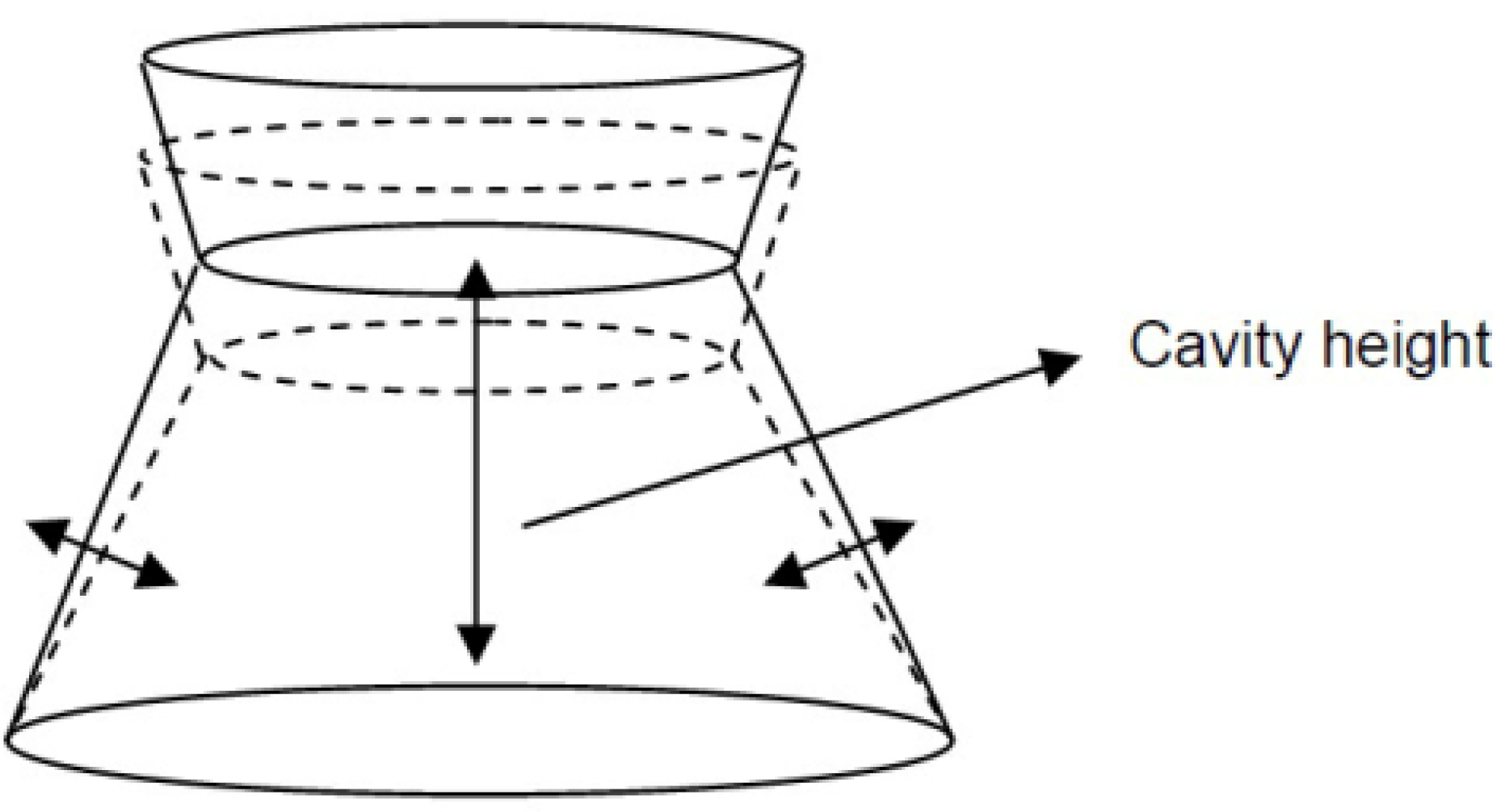
| Cavity Height [cm] | 15 |
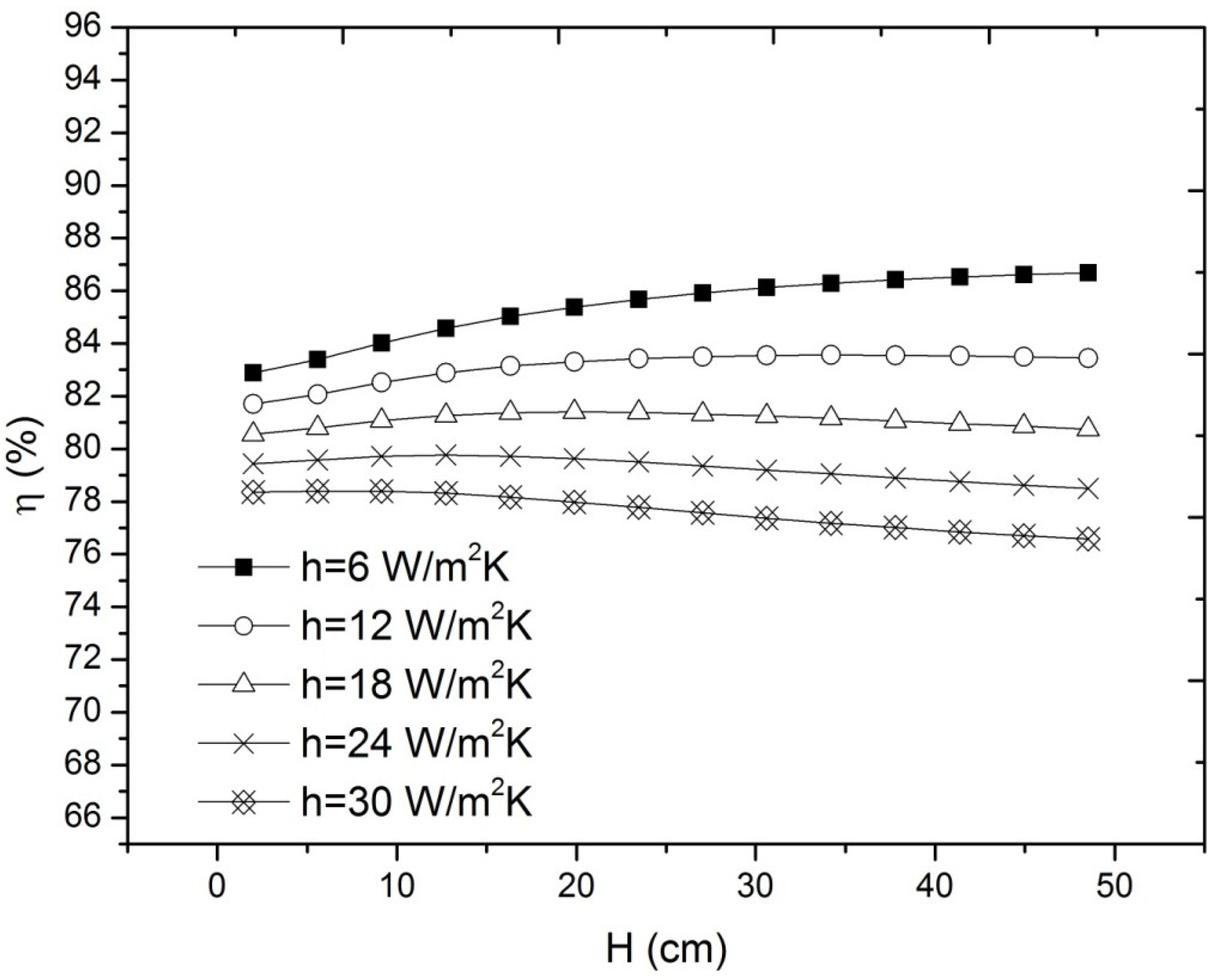
3.1. Finite Differences


| Aperture Height Analysis | h = 6 W/m2K | h = 12 W/m2K | h = 18 W/m2K | h = 24 W/m2K |
|---|---|---|---|---|
| Rap = 8 cm | 24 | 9 | 5 | <5 |
| Rap = 10 cm | 41 | 19 | 13 | 7 |
| Rap = 12 cm | >45 | 34 | 20 | 12 |

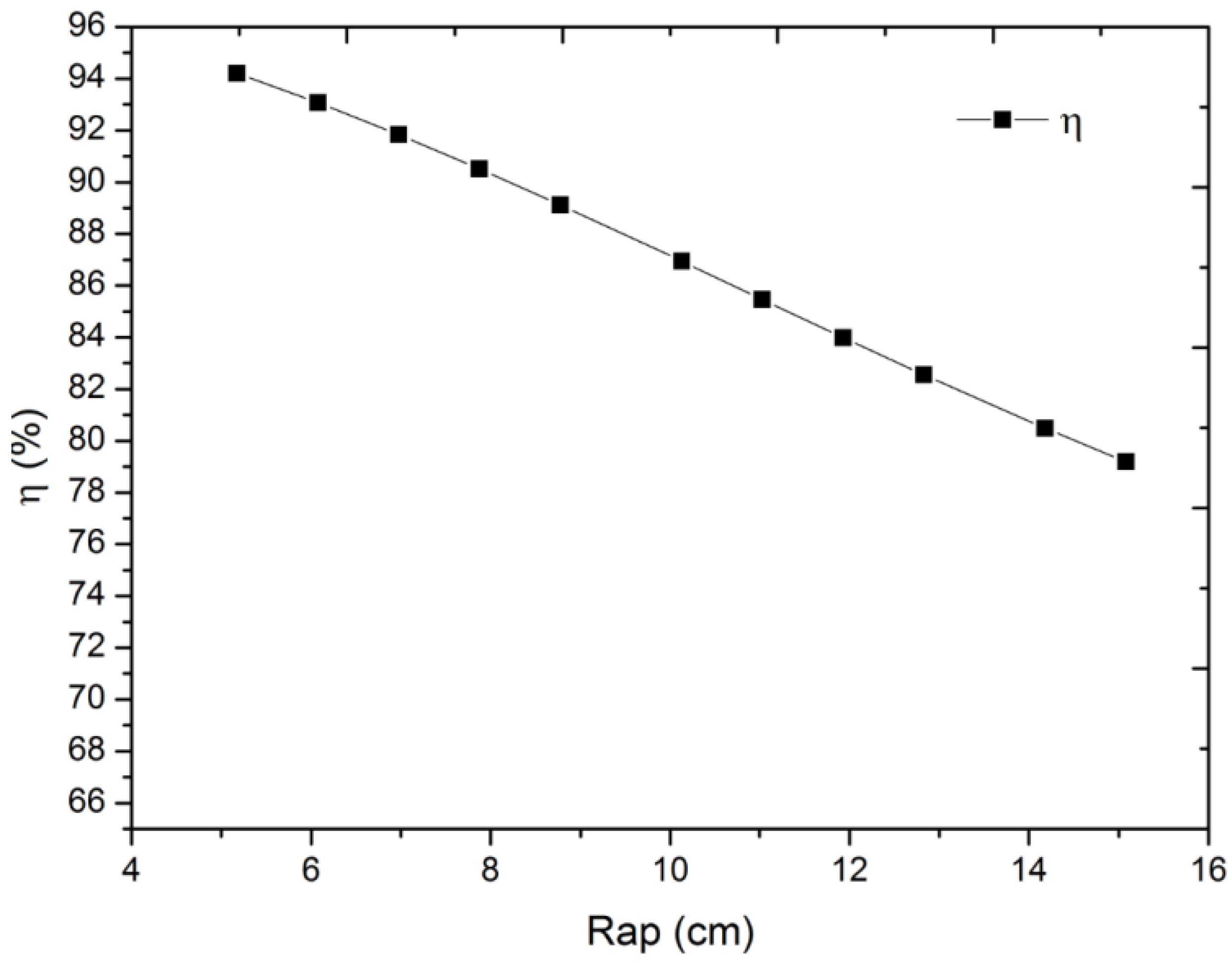
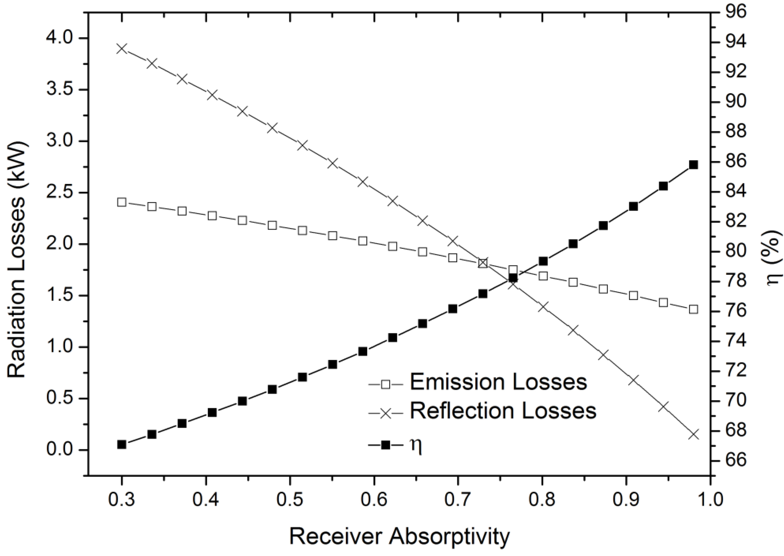
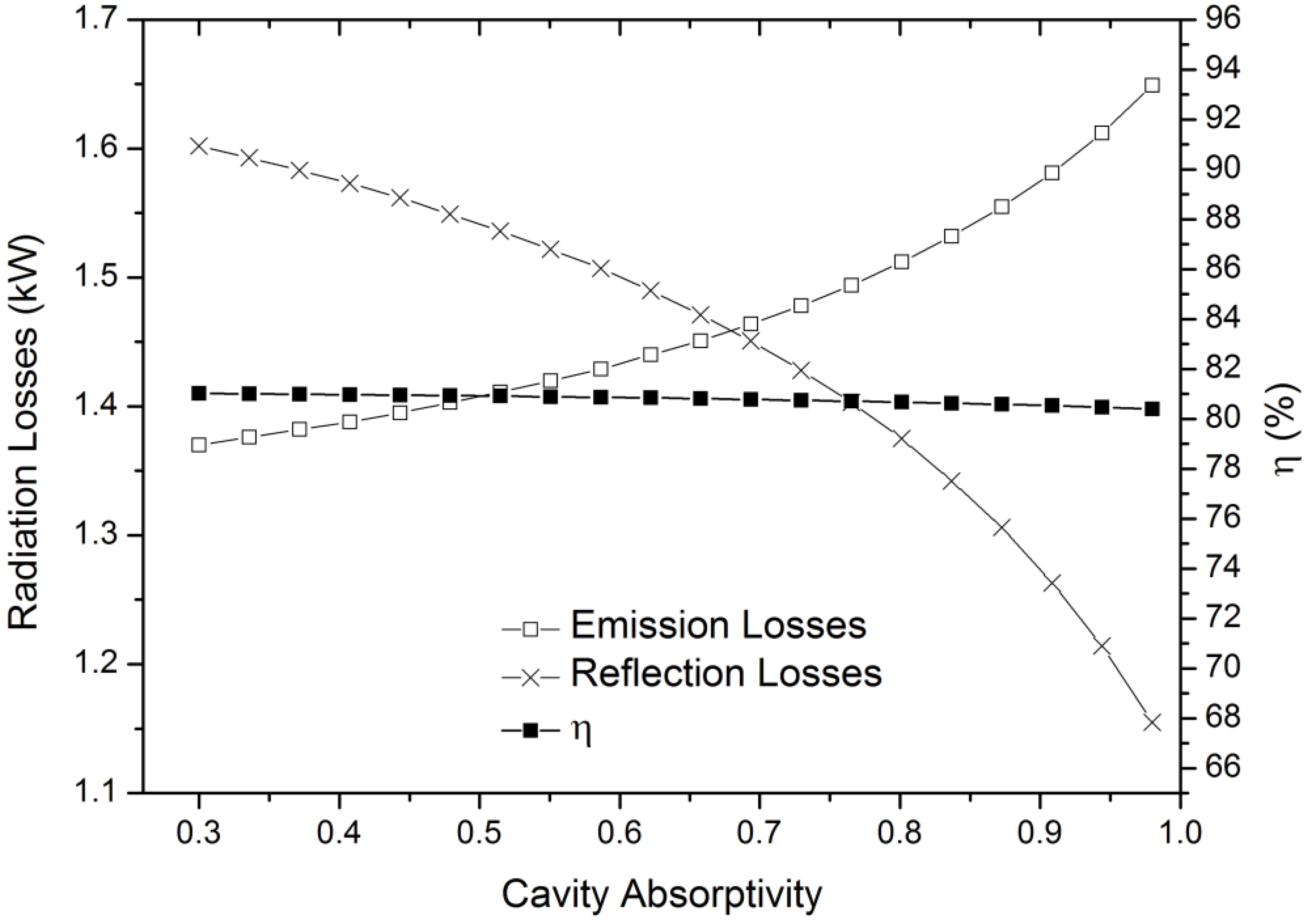
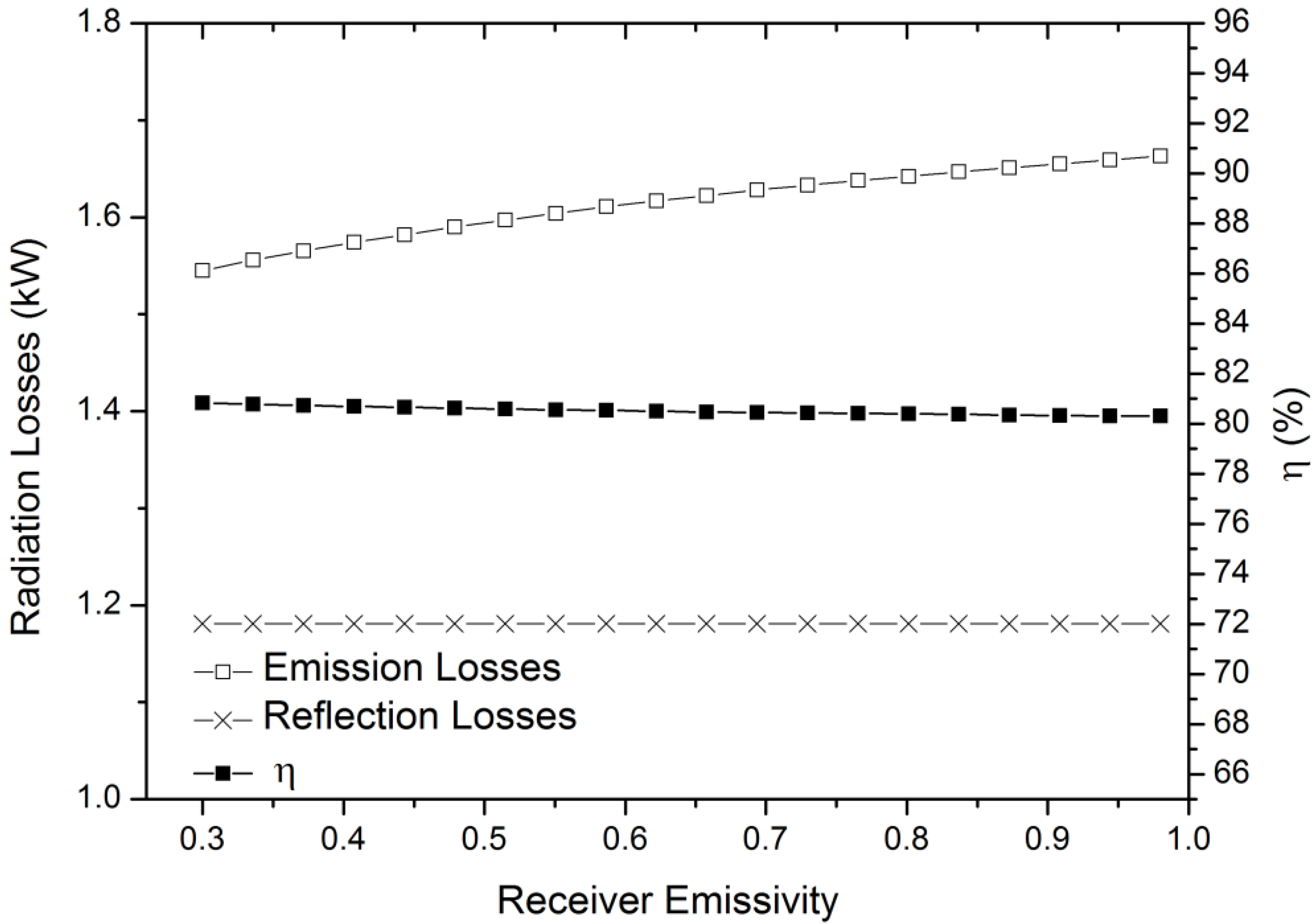
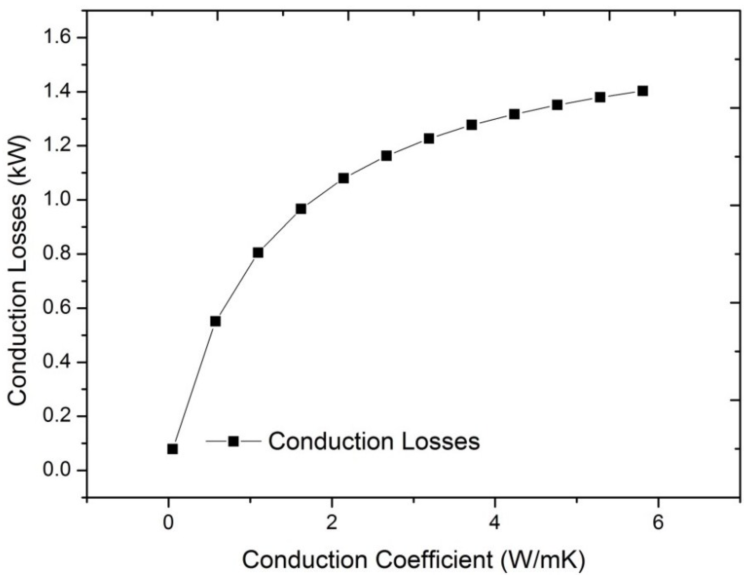
3.2. Optimal Material Properties


4. Conclusions
Acknowledgments
Author Contributions
Nomenclature
| A | Area |
| F | View factor |
| H | Aperture cavity height |
| J | Radiosity |
| q | Heat transfer |
| R | Radius |
| T | Temperature |
| x | Ratio between dish radius and distance between dishes |
| X | Coefficient to solve view factor between two coaxial and parallel dishes |
Greek symbols
| δ | Distance between dish 1 and dish 2 |
| ε | Emissivity |
| η | Efficiency |
| λ | Wavelength |
| ρ | Reflectivity |
| σ | Stefan-Boltzmann constant (=5.670373 × 10⁻⁸ W·m−2·K−4) |
| φ | Incident solar flux |
Subscripts
| ap | Aperture |
| d1 | Dish 1 (view factor calculation) |
| d2 | Dish 2 (view factor calculation) |
| ec | Emission spectrum (thermal radiation) |
| i | Surface “i” |
| j | Surface “j” |
Units
| cm | Centimeters |
| K | Kelvin |
| kW | Kilowatts |
| kWt | Thermal Kilowatts |
| m | Meters |
| m2 | Square meters |
| W | Watts |
| µm | Micrometer |
Conflicts of Interest
References
- Bravo, Y.; Carvalho, M.; Serra, L.M.; Monné, C.; Alonso, S.; Moreno, F.; Muñoz, M. Environmental evaluation of dish-Stirling technology for power generation. Sol. Energy 2012, 86, 2811–2825. [Google Scholar]
- Monné, C.; Bravo, Y.; Moreno, F. Analysis of a solar dish-Stirling system with hybridization and thermal storage. Int. J. Energy Environ. Eng. 2014, 5, 1–5. [Google Scholar] [CrossRef]
- Bravo, Y.; Monné, C.; Bernal, N.; Carvalho, M.; Moreno, F.; Muñoz, M. Hybridization of solar dish-stirling technology: Analysis and design. Environ. Prog. Sustain. Energy 2014, 33, 1459–1466. [Google Scholar]
- Hogan, R.E., Jr. AEETES—A solar reflux receiver thermal performance numerical model. Sol. Energy 1994, 52, 167–178. [Google Scholar] [CrossRef]
- Diver, R.B. Reflux solar receiver design considerations. In Proceedings of ASME-JSES-KSES International Solar Energy Conference, Maui, HI, USA, 4–8 April 1992.
- Shuai, Y.; Xia, X.-L.; Tan, H.-P. Radiation performance of dish solar concentrator/cavity receiver systems. Sol. Energy 2008, 82, 13–21. [Google Scholar] [CrossRef]
- Li, Z.; Tang, D.; Du, J.; Li, T. Study on the radiation flux and temperature distributions of the concentrator-receiver system in a solar dish/Stirling power facility. Appl. Therm. Eng. 2011, 31, 1780–1789. [Google Scholar] [CrossRef]
- Müller, R.; Steinfeld, A. Band-approximated radiative heat transfer analysis of a solar chemical reactor for the thermal dissociation of zinc oxide. Sol. Energy 2007, 81, 1285–1294. [Google Scholar] [CrossRef]
- Nadal, R.P.; Moll, V.M. Optical analysis of the fixed mirror solar concentrator by forward ray-tracing procedure. J. Sol. Energy Eng. 2012, 134. [Google Scholar] [CrossRef]
- Nepveu, F.; Ferriere, A.; Bataille, F. Thermal model of a dish/Stirling systems. Sol. Energy 2009, 83, 81–89. [Google Scholar]
- Montiel Gonzalez, M.; Hinojosa Palafox, J.; Estrada, C.A. Numerical study of heat transfer by natural convection and surface thermal radiation in an open cavity receiver. Sol. Energy 2012, 86, 1118–1128. [Google Scholar] [CrossRef]
- Natarajan, S.K.; Reddy, K.S.; Mallick, T.K. Heat loss characteristics of trapezoidal cavity receiver for solar linear concentrating system. Appl. Energy 2012, 93, 523–531. [Google Scholar] [CrossRef]
- Teichel, S.H.; Feierabend, L.; Klein, S.A.; Reindl, D.T. An alternative method for calculation of semi-gray radiation heat transfer in solar central cavity receivers. Sol. Energy 2012, 86, 1899–1909. [Google Scholar] [CrossRef]
- Martinek, J.; Weimer, A.W. Evaluation of finite volume solutions for radiative heat transfer in a closed cavity solar receiver for high temperature solar thermal processes. Int. J. Heat Mass Transf. 2013, 58, 585–596. [Google Scholar] [CrossRef]
- Meiser, S.; Kleine-Büning, C.; Uhlig, R.; Lüpfert, E.; Schiricke, B.; Pitz-Paal, R. Finite Element Modeling of Parabolic Trough Mirror Shape in Different Mirror Angles. J. Sol. Energy Eng. 2013, 135. [Google Scholar] [CrossRef]
- Wu, S.-Y.; Xiao, L.; Cao, Y.; Li, Y.R. Convection heat loss from cavity receiver in parabolic dish solar thermal power system: A review. Sol. Energy 2010, 84, 1342–1355. [Google Scholar] [CrossRef]
- Prakash, M.; Kedare, S.B.; Nayak, J.K. Determination of stagnation and convective zones in a solar cavity receiver. Int. J. Therm. Sci. 2010, 49, 680–691. [Google Scholar] [CrossRef]
- Xiao, L.; Wu, S.Y.; Li, Y.R. Numerical study on combined free-forced convection heat loss of solar cavity receiver under wind environments. Int. J. Therm. Sci. 2012, 60, 182–194. [Google Scholar] [CrossRef]
- Wu, S.Y.; Guo, F.H.; Xiao, L. Numerical investigation on combined natural convection and radiation heat losses in one side open cylindrical cavity with constant heat flux. Int. J. Heat Mass Transf. 2014, 71, 573–584. [Google Scholar] [CrossRef]
- F-Chart Software. Available online: http://www.fchart.com/ (accessed on 27 January 2015).
- Abate, S.; Barberi, R.; Desiderio, G.; Lombardo, G. Solar Radiation Heat Absorber for a Stirling Motor. World Patent WO2012/016873 A1, 9 February 2012. [Google Scholar]
- Li, Y.; He, Y.; Wang, W. Optimization of solar-powered Stirling heat engine with finite-time thermodynamics. Renew. Energy 2011, 36, 421–427. [Google Scholar] [CrossRef]
- Incropera, F.P.; DeWitt, D.P. Fundamentals of Heat and Mass Transfer, 4th ed.; John Wiley & Sons: New York, NY, USA, 1996; pp. 633–783. [Google Scholar]
- Mills, A.F. Transferencia de Calor; Irwin: Madrid, Spain, 1995; pp. 129–254. (In Spanish) [Google Scholar]
- Cleanergy. Available online: http://www.cleanergy.com (accessed on 5 June 2014).
© 2015 by the authors; licensee MDPI, Basel, Switzerland. This article is an open access article distributed under the terms and conditions of the Creative Commons Attribution license (http://creativecommons.org/licenses/by/4.0/).
Share and Cite
Gil, R.; Monné, C.; Bernal, N.; Muñoz, M.; Moreno, F. Thermal Model of a Dish Stirling Cavity-Receiver. Energies 2015, 8, 1042-1057. https://doi.org/10.3390/en8021042
Gil R, Monné C, Bernal N, Muñoz M, Moreno F. Thermal Model of a Dish Stirling Cavity-Receiver. Energies. 2015; 8(2):1042-1057. https://doi.org/10.3390/en8021042
Chicago/Turabian StyleGil, Rubén, Carlos Monné, Nuria Bernal, Mariano Muñoz, and Francisco Moreno. 2015. "Thermal Model of a Dish Stirling Cavity-Receiver" Energies 8, no. 2: 1042-1057. https://doi.org/10.3390/en8021042