A Novel Ground Fault Non-Directional Selective Protection Method for Ungrounded Distribution Networks

Abstract

This paper presents a new selective and non-directional protection method to detect ground faults in neutral isolated power systems. The new proposed method is based on the comparison of the rms value of the residual current of all the lines connected to a bus, and it is able to determine the line with ground defect. Additionally, this method can be used for the protection of secondary substation. This protection method avoids the unwanted trips produced by wrong settings or wiring errors, which sometimes occur in the existing directional ground fault protections. This new method has been validated through computer simulations and experimental laboratory tests.

1. Introduction

Distribution power systems are equipped with sophisticated protection devices to keep them safe from overloads, short circuits, voltage sags and drops and, in general, any operation conditions out of rated values, something which might represent a clear danger not only to the facilities, but also to the power system operation. Although in some countries the distribution networks can reach 150 kV [1], the isolated distribution networks worldwide are normally classified in voltage levels from 1 kV to 45 kV and have the advantage that a single phase ground fault (SPGF) of the system does not produce high ground fault overcurrents; therefore, the whole system remains operational. In this case, the power system must be designed to withstand high transient and permanent steady state over voltages, so its use is generally restricted to low and medium voltage systems.

These systems enjoy low current values when a SPGF happens. Such ground fault currents are not related to the amount of power generated or distributed as they are only produced by the capacitance distributed in all power elements that form such neutral ungrounded network. Therefore, all kind of possible distributed generation units (DGs) connected to this kind of networks are not exposed to high currents values when a SPGF is taking place. These kind of neutral ungrounded networks are designed to be able to withstand over voltages up to190% of rated voltage value over 8 h [2,3].

A SPGF at one line of an isolated power system makes capacitive currents flow through all the lines, and the voltages of the phases without defect are increased up to the phase-to-phase voltage level—that is an overvoltage of 173%.

Lines without ground faults contribute with their own capacitive current flowing from the busbars to the fault. The direction of the residual current in the line with ground fault is opposite to the direction of the capacitive currents in the lines without ground defect. Under such circumstances, the existing protection devices use directional ground fault criterion, measuring the residual current, the residual voltage and the phase shift between them.

This relay provides ground fault detection, but presents important operational difficulties that could imply unwanted tripping commands. Such difficulties are related to substations that cannot be removed from service, while the commissioning jobs must be developed; therefore, there is no chance to test the directional ground fault protection relays using primary injection tests. Secondary tests are always satisfactory but they are not enough to grant the correct behaviour of the protection relay when there is a real ground defect, and in addition, some wrong tripping actions happen from time to time.

The new proposed method is based on the comparison of the rms value of the residual current of all the lines connected to a bus. As it is a non-directional method, errors in the polarity of the connections of the current transformers have no influence on its operation. A wrong setting definition is also eliminated because of its comparison principle. These two last aspects normally drive directional ground fault protections to make unintended tripping commands.

This paper first describes, in Section 2, the state of the art of fault detection in neutral isolated power systems. Section 3 describes the principle of operation of the new non-directional method to detect single phase ground faults at isolated networks. ATP simulation results and laboratory test results are shown in Section 4 and Section 5, respectively. Finally, in Section 6, the main conclusions are listed.

2. State of the Art

The use of symmetrical components [4] can also be applied to study the ground fault capacitive current values. Some research works have obtained excellent results using hybrid compensation methods [5,6] and their use, although it is not widespread employed by distribution electrical companies, is perfectly applicable to neutral ungrounded networks whereas other investigation works build different algorithms to determine the ground fault current value [7].

There are several methods to detect SPGF at neutral ungrounded networks. Some of them use compensation factors [8] for the residual voltage whereas others study the shape of charge-voltage curves when a ground fault is present [9]. Other options include the installation of current and voltage sensors along the medium voltage network and install management software to detect the feeder with defect [10,11] after the protection systems have tripped the circuit breaker corresponding to the feeder with ground defect.

New algorithms [12] and methods that compare the ground fault currents to new reference current magnitude [13] have been also evaluated. Open research that might be applied to the detection and localization of ground faults is described in [14]. Recently, the use of the Wavelet analysis [15,16,17] has achieved excellent results in fault detection. Once the fault has been detected, the different protection methods can give an alarm or a tripping command in order to avoid damage to the power system elements, and remove from service the zone with fault condition, providing selectivity. Normally, the distribution companies use two protection relays to detect and clear the SPGF in neutral ungrounded networks.

Figure 1. Residual current distribution in an underground neutral undergrounded system with ground fault at F in phase “c” of Line 1.

Figure 1. Residual current distribution in an underground neutral undergrounded system with ground fault at F in phase “c” of Line 1.

The first one is a residual over voltage protection relay (ANSI 59N). This protection relay only evaluates the residual voltage at the busbars of the substation, not the phase voltage values [18]. This residual voltage is normally measured through three voltage transformers in open delta connection installed at the medium voltage busbars of the substation. The worst drawback of this way of detection is that the location of the fault is not possible to determine, as the residual voltage is present in the entire power system. In fact, depending of the distribution operator company, this type of protection can be used to signal an alarm or trip the entire busbar system and remove from service all lines connected to such busbar system. The trip of the entire busbar system is unacceptable due to a SPGF in any line.

The second protection relay used is the ground directional protection relay (GDPR) [19,20]. This protection is based on the different directions of the residual currents in case of ground fault. The residual current in the line with ground defect has an opposite direction than in the rest of the lines, as shown in Figure 1. This protection only has to trip in case of residual current circulating in the appropriate direction. So in order to distinguish the line with ground defect, it is necessary to measure the residual current direction at every line connected to the busbars of the substation. For such purpose, a directional ground fault protection relay is installed at every line.

The evaluation of the direction of the residual current needs the measurement of the residual voltage as reference vector. This residual voltage is obtained in the same way as described before in the use of the residual over voltage protection (ANSI 59N). Therefore, when the ground fault residual current and the residual voltage are over their setting values, a directional comparison between the ground fault residual current and the residual voltage is done. In function of the angle between them, a tripping command is performed.

The maximum sensitivity characteristic angle between the residual voltage U₀ and the residual current I₀ can be adjusted in the directional protection relays as a function of the neutral point connection. These protections relays are more expensive than the residual overvoltage relays, as they have to manage voltages, currents and develop a directional comparison.

This directional protection system is not free of problems. Sometimes, when there is a ground fault in one line, there are unwanted trips in other lines caused by a wrong setting or wiring errors in their respective ground fault directional protection relays. These wrong tripping commands cannot be avoided in some installations where a primary test injection is not possible because the power supply cannot be switched off; In this case, neither a minimum residual voltage nor a residual current can be injected in the directional relays, and only secondary tests could be performed.

Under such circumstances, when a real ground defect happens, the correct behaviour of the directional protection relay cannot be granted. Therefore, only when a ground fault happens, is it possible to detect an error in the settings or in the wiring of the directional ground protection relays.

Commissioning engineers have to cope with the right identification of the polarity of the VT’s and CT’s wired to the GDPR as its manufacturer indicates, the right tripping direction indicated by the GDPR manufacturer, the right tripping angle between residual voltage U₀ and the residual current I₀ and the right current circulations when there is a SPGF.

These last drawbacks related to the GDPR make the use of other protection systems interesting, which could be set in operation without primary test injections and provide full protection with total selectivity against ground faults to all the lines connected to the same busbars in any substation.

In Figure 2, the circulating currents are shown in all the lines in an underground power system when a ground defect happens at F location at phase “c” in Line 1. At every phase of the three lines, its own capacitive current is circulating towards the fault point F except the capacitive current components at the phase “c” in the entire power system because they are short-circuited. Therefore, the capacitive current measured by the ring core current transformers CT that embrace the three phases at Lines 2 and 3 are the sum of the capacitive currents of their phases; in Line 2 it is I_E2 = I_CA,2 + I_CB,2, and in Line 3 it is I_E3 = I_CA,3 + I_CB,3. These currents I_E2 and I_E3 have direction from the busbars to the line.

Figure 2. Residual current distribution in a three line neutral ungrounded system with ground fault at F in phase “c” of Line 1.

Figure 2. Residual current distribution in a three line neutral ungrounded system with ground fault at F in phase “c” of Line 1.

However, the capacitive current measured by the ring core current transformer (CT) in Line 1 is the sum of the capacitive currents I_E2 and I_E3 with direction from the fault point F to the busbars. The capacitive current I_E1 flows back and forth through the CT of the Line 1, so it is neglected. Every ground fault directional protection relay installed per line, reads the residual voltage U₀ at the busbars obtained from the voltage transformers (VT) in open-delta connection and the currents I_p1, I_p2 and I_p3.

These I_p1, I_p2 and I_p3 currents are the respective capacitive currents in primary side of Lines 1, 2 and 3, referred to the secondary side through the current transformer ratio TR of the ring core current transformers CT used.

In case of having an outdoor power system with feeders, there must be three current transformers installed in each feeder in Holmgreen connection to be able to read the ground fault current as it is indicated in Figure 3. In Figure 4, Figure 5 and Figure 6 the measurements of residual voltage and current in the three GDPR are illustrated. Only when their settings and the wirings are correct, GDPR in Line 1 is the only one GDPR which trips when a SPGF happens in Line 1.

From Figure 4, Figure 5 and Figure 6 it is seen that the Line 1 with ground fault has residual current 3I_0,1 leading the residual voltage 90°, whereas in Lines 2 and 3 without ground defect, their residual currents 3I_0,2 and 3I_0,3 lag the residual voltage. It can be concluded that when the ground fault directional relays are well adjusted and wired, their performance is quite good, but in some situations, such as when a new relay is going to be installed or maintenance works do not allow making primary injection to test the protection relays, their behavior is committed. A new protection method that avoids such maintenance problems and the difficulty of checking the performance of the relays at any time with full effectiveness is described in this article.

Figure 3. Current transformers connected in Holmgreen connection.

Figure 3. Current transformers connected in Holmgreen connection.

Figure 4. Vector diagram. Residual voltage and current in Line 1 with ground defect.

Figure 4. Vector diagram. Residual voltage and current in Line 1 with ground defect.

Figure 5. Vector diagram. Residual voltage and current in Line 2 with ground defect in Line 1.

Figure 5. Vector diagram. Residual voltage and current in Line 2 with ground defect in Line 1.

Figure 6. Vector diagram. Residual voltage and current in Line 3 with ground defect in Line 1.

Figure 6. Vector diagram. Residual voltage and current in Line 3 with ground defect in Line 1.

3. Principle of Operation of the New Selective Ground Fault Detection Technique

Before explaining the new principle of operation, the circulating of defect and capacitive currents when there is a SPGF in an isolated network is explained in detail.

In cases of ground fault, the capacitive currents of all the n−1 lines without defect will circulate to the line with ground defect. On the other hand, in any line free of defects, only its own capacitive current I_E will flow as indicated in Figure 1. This can be expressed as follows:

$$\begin{array}{c}\text{Residual} \text{capacitive} \text{current} \text{in} \text{line} \text{with} \text{no} \text{ground} \text{defect}: I_{E,NGD}=I_E(\mathrm{A})\\ \text{Residual} \text{capacitive} \text{current} \text{in} \text{line} \text{with} \text{ground} \text{defect}: I_{E,WGD}={\displaystyle \sum _1^{n-1}}{I}_{E,NGD}(\mathrm{A})\end{array}$$

(1)

where I_E,NGD is the capacitive current I_E of any of the n–1 lines with no ground defect (NGD), whereas the capacitive current of the line with ground defect (WGD), I_E,WGD, is the sum of the n−1 capacitive currents I_E of the rest of the lines with no ground defect.

When a power system has a ground fault at any undergrounded line “i” in phase “a” for example, the modules of the capacitive currents I_CBi and I_CCi of phases “b” and “c” are given by the equation:

$$\begin{array}{c}{I}_{CBi}=I_{CCi}=\frac{\sqrt{3}·U_{phase}}{X_C}=\sqrt{3}·U_{phase}·j·2·\pi ·f·C_{ph}·L(\mathrm{A})\\ X_C=\frac{1}{j·2·\pi ·f·C_{ph}}\end{array}$$

(2)

where U_phase is the nominal phase-to-neutral voltage of the power system, X_C is the capacitive ground impedance value, f is the frequency of the power system, C_ph is the capacitance per length unit of one phase and L is the length of the line or cable. The larger the capacitance, the greater capacitive current the line will have. Normally this capacitance C_ph is given in F/km. When the power system is free of ground faults, the capacitive currents in any line have the same value in all its phases.

Figure 2 shows an example of the circulating currents in all the lines in an underground 20 kV power system when a SPGF happens in Line 1, phase “c” in point F. The lengths of the Lines 1, 2 and 3 are 6, 10 and 8 km respectively; each line has one single cable per phase with a capacitance to earth 0.25 μF/km which represents about 1.57 A/km/phase. These data represent in Line 1 a current value of I_E1 = 18.84 A, in Line 2 it is I_E2 = 31.407 A and in Line 3 I_E3 = 25.122 A. The current I_E1 circulates back and forth through the CT installed in Line 1 so it does not affect in the current value measured whereas both currents I_E2 and I_E3 circulate from busbars to the fault point F. Therefore, the circulating currents measured by the three CTs are: 56.53 A in Line 1 with direction from the fault point F to the busbars; 31.40 A in Line 2 with direction from the busbars to the fault point, and 25.12 A in Line 3 from the busbars to the fault point.

The proposed method is based on the comparison of the rms values of the residual current of all the lines connected to a bus. Figure 2 shows how Line 1 with SPGF has the highest residual current compared to the residual currents in Lines 2 and 3 without ground defect. An additional condition for verifying the presence of a ground fault in the power system should be the evaluation of a minimum residual voltage to avoid undesirable tripping commands [21]. Therefore, in a power system with more than two lines, in the case of a ground fault, the line with ground defect would have the biggest residual current of all the lines.

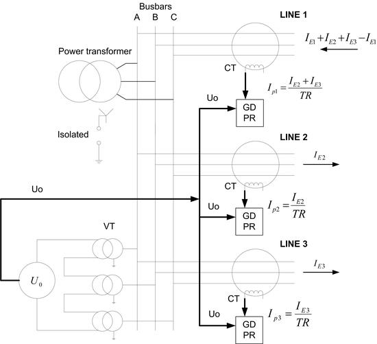
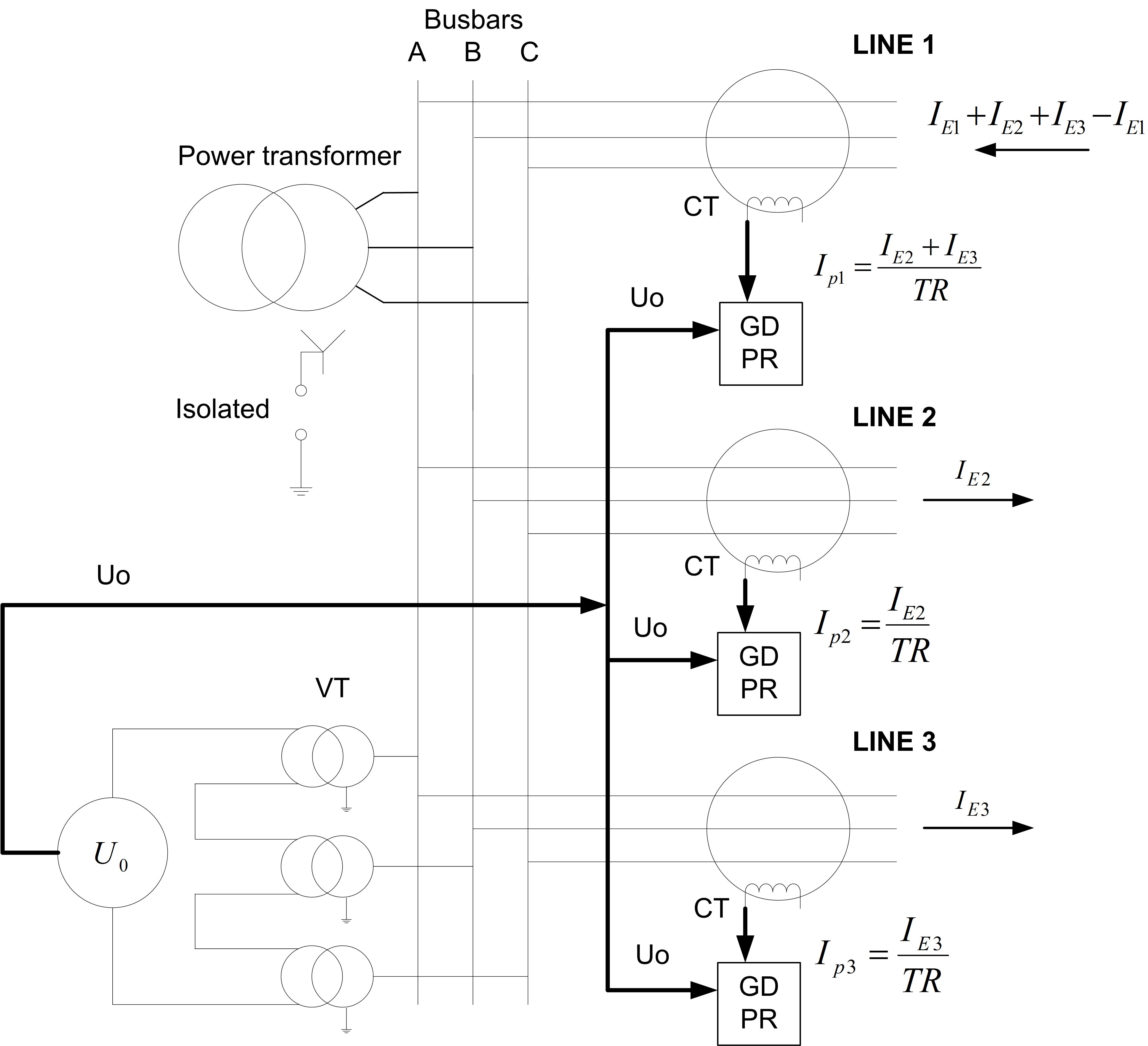
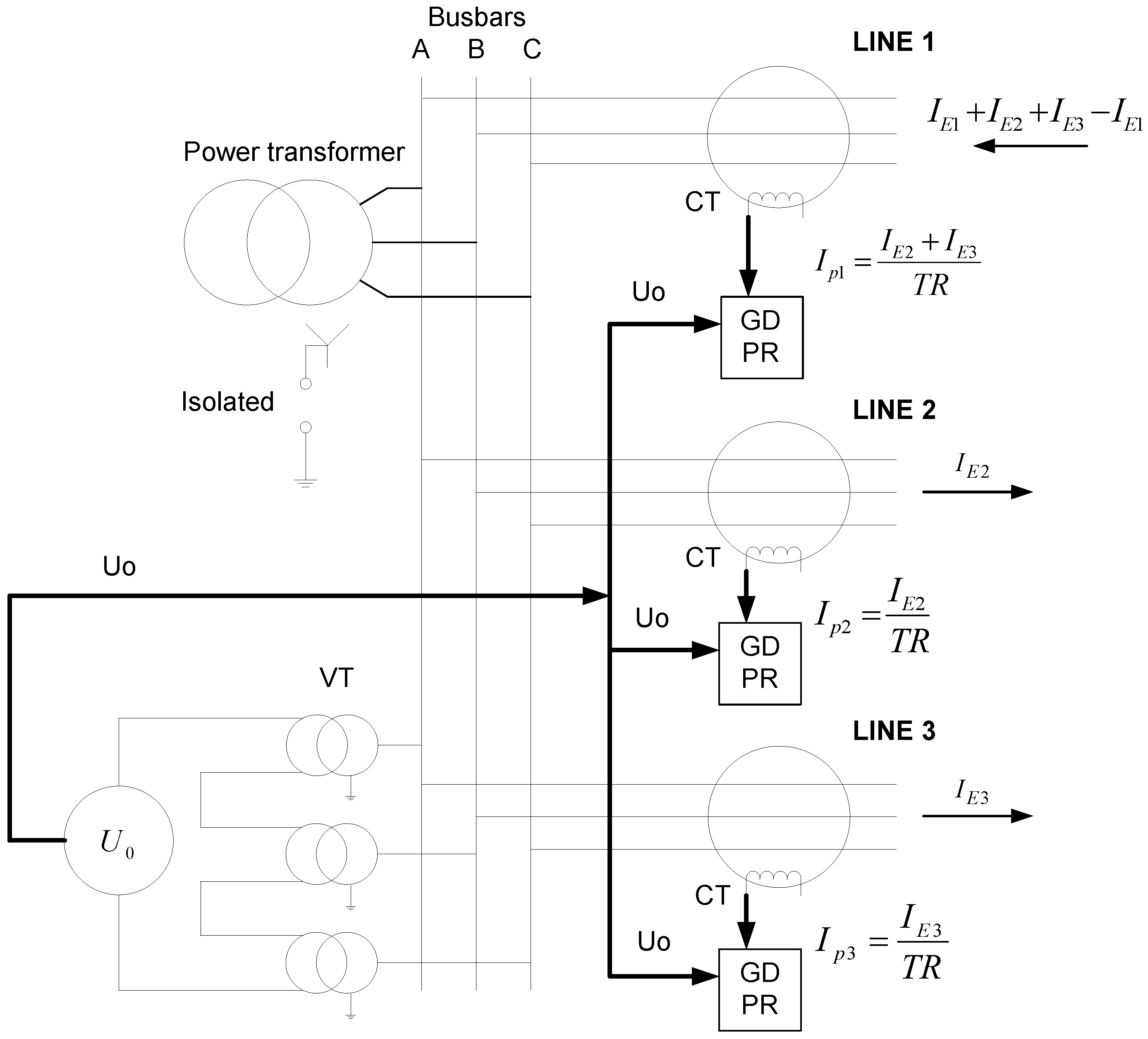
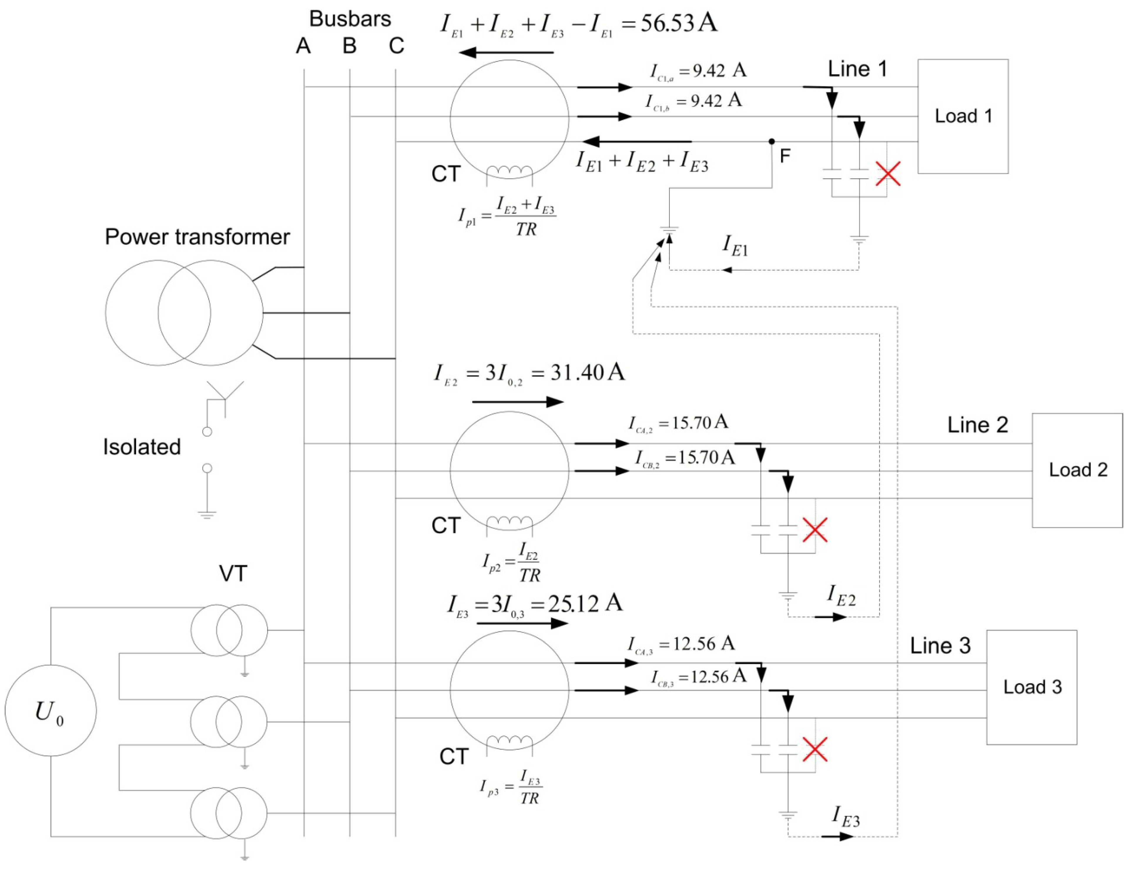
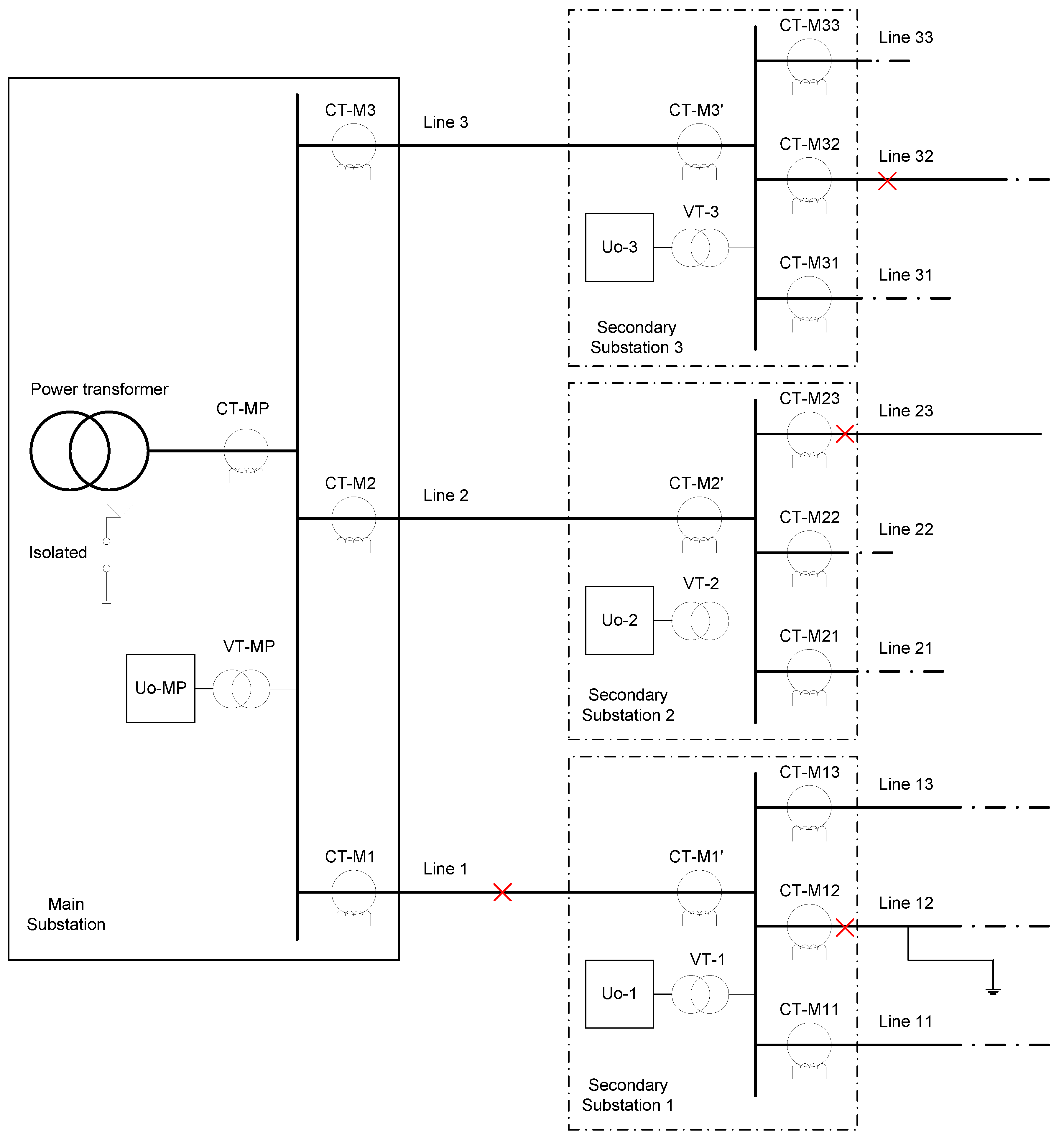
3.1. Ground Fault Detection Method for Main Substations

At main substations fed directly by power transformers, in the line that has a SPGF, a residual current can be measured that corresponds to the addition of the capacitive currents of the rest lines in service without ground fault. In each of the healthy lines, the residual currents correspond to their own capacitive currents. The line with SPGF is easily detectable in this type of substation by comparing the rms values of the residual currents. The line with the highest residual current is the line that has a ground fault. As shown in Figure 2, the line with ground defect (Line 1) has a residual current corresponding to the sum of the capacitive currents of the other lines: I_E2 + I_E3, while in Lines 2 and 3, the residual currents are I_E2 and I_E3, respectively.

3.2. Ground Fault Detection Algorithm for Secondary Substations

In power systems with one main substation and several secondary substations, the new non-directional method should be implemented in the main substation and in the secondary substations. Secondary substations correspond to those that have incoming feeders/lines and outgoing feeders/lines connected at the same busbars and can be considered as a single bus in the network.

As shown in Figure 7, where there are one main substation and three secondary substations. In case of a SPGF, if the described method to detect ground faults is used in the secondary substations, tripping commands will take place at all secondary substations simultaneously. The reason is that when there is a ground fault, defect currents flow at every single line of the network. According to this new method presented for main substations, the line with the highest residual current at every substation will be tripped, and this line could be the line that has a ground fault or simply the longest line of the substation. For instance, in the power system represented in Figure 7, in case of a fault in Line 12, not only the outgoing Line 12 would be tripped, but also the longest lines at secondary substations 2 and 3 (Line 23 and Line 32 respectively). Therefore, an important part of the power system will be disconnected inappropriately. This fact is considered by the proposed method in the specific case of secondary substations. The method requires choosing the principal line or lines that supply electrical power to the busbars, as well as the outgoing lines that set out from such busbars. Once this selection is defined, the procedure to determine where the fault is to check two conditions.

Figure 7. Highest ground fault currents at isolated network with secondary substations. Ground fault at Line 12.

Figure 7. Highest ground fault currents at isolated network with secondary substations. Ground fault at Line 12.

The first condition is to detect a SPGF in the system by the measurement of the residual voltage U₀. If the value of this residual voltage U₀ is above a previous setting value, the next step is triggered. Now the defect current rms values due to the capacitance of the system at every incoming and outgoing line at any secondary substation are read out and evaluated. The algorithm checks if the sum of all outgoing rms residual current values is equal to the sum of all incoming rms residual current values in a secondary substation. If so, the fault is not taking place at any outgoing line of that secondary substation. But if this second condition is not fulfilled at any secondary substation, the new system will trip the line with highest defect current at that secondary substation. The algorithm of the method is shown in Figure 8.

Figure 8. Secondary substation. Algorithm for SPGF detection.

Figure 8. Secondary substation. Algorithm for SPGF detection.

3.3. Examples of Application of the New Method

The working principle of the new method is evaluated in two different scenarios:

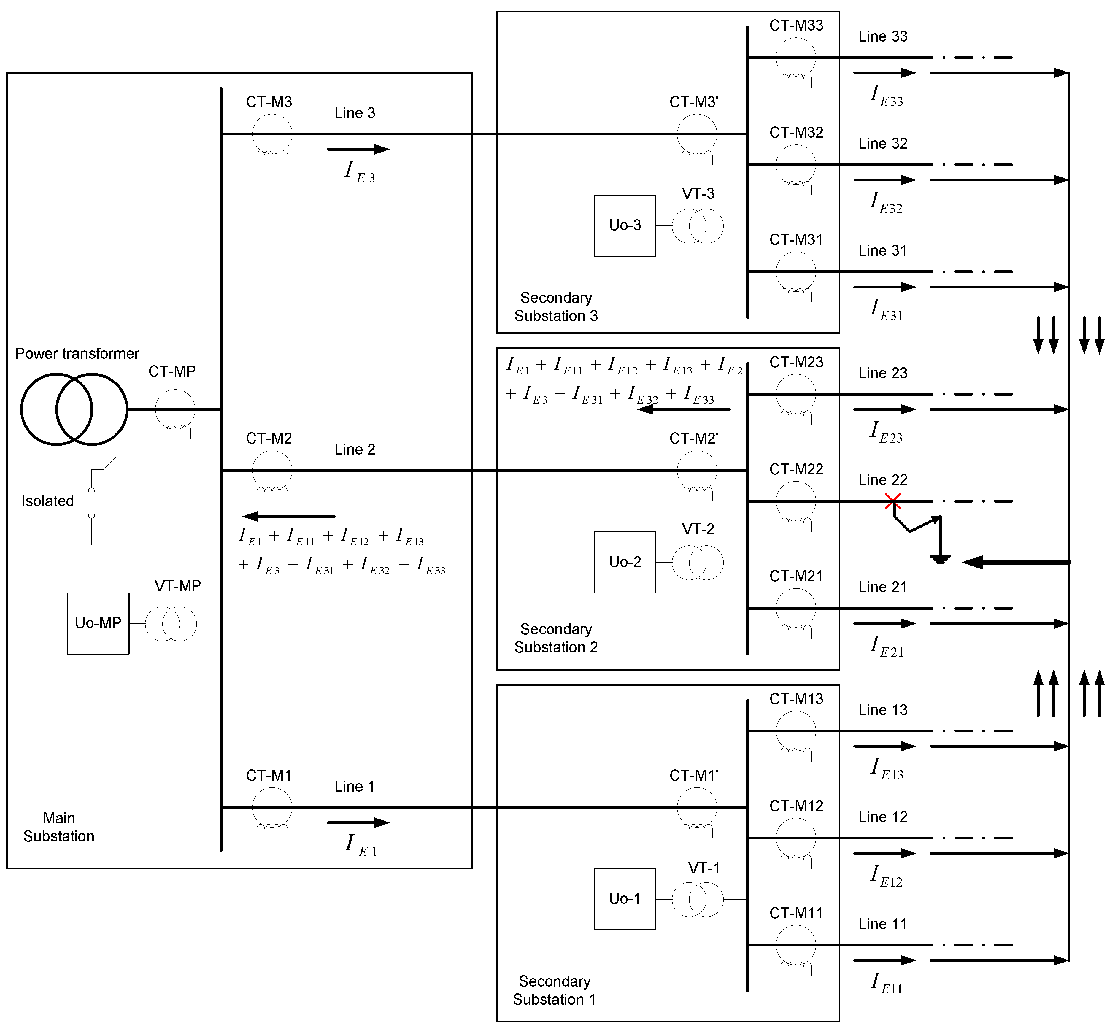
3.3.1. Ground Fault in an Outgoing Line of any Secondary Substation

Let us consider a network composed of a main substation and three secondary substations, shown in Figure 9, where a SPGF has occurred in Line 22. The measurements of the current transformers of the main and secondary lines are summarized in Table 1. In this example, using the appropriated criteria for a secondary substation, the new selective ground fault method operates as follows:

-

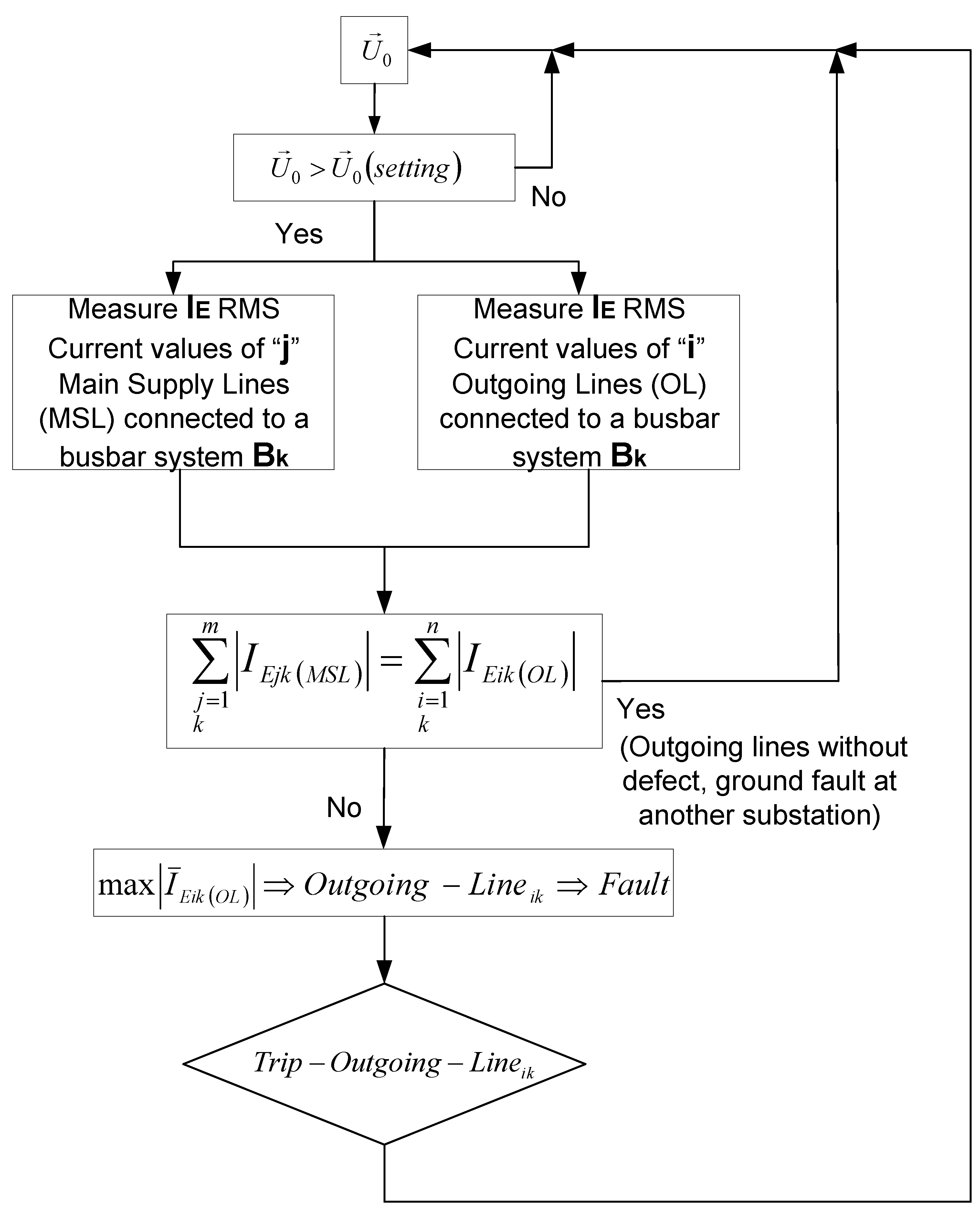
When the residual voltage level is over the setting value, the residual currents are evaluated.

-

At secondary substation 1, the defect current measured at the incoming Line 1 by the current transformer CT-M1’ has an rms value equal to the sum of the rms values of the defect currents measured at the outgoing Lines 11, 12 and 13 by their respective current transformers CT-M11, CT-M12 and CT-M13. Using the second condition criterion, it is concluded that the fault is not located at any of these outgoing lines. The same conclusion can be made for secondary substation 3.

-

At secondary substation 2, the defect current measured at the incoming Line 2 by its current transformer CT-M’ has a different rms value from the sum of the rms values of the defect currents measured at the outgoing Lines 21, 22 and 23 by their respective current transformers CT-M21, CT-M22 and CT-M23. Now, as the highest defect current is measured at outgoing Line 22, the conclusion from employing the second condition criteria is that the fault is in such line.

-

At the main substation, the defect current measured at the outgoing Line 2 by its current transformer CT-M2 has the highest rms value of all the outgoing currents in Lines 1, 2 and 3 measured by their respective current transformers CT-M1, CT-M2 and CT-M3. The new method would switch off Line 2as a consequence of the first condition criterion.

To avoid a tripping order at the outgoing Line 2 at the main substation before a tripping order at the outgoing Line 22, there must be a time delay between such commands. Tripping orders at secondary substations must be quicker than the main substation ones to provide selectivity.

Figure 9. Highest ground fault currents at neutral undergrounded network with secondary substations. SPGF at Line 22.

Figure 9. Highest ground fault currents at neutral undergrounded network with secondary substations. SPGF at Line 22.

Table 1. Residual current measurements. Ground fault at Line 22—Phase “a”—rms current value (A).

Main station		Secondary substation II
CT-MP	0	CT-M2’	IE1 + IE11 + IE12 + IE13 + IE3 + IE31 + IE32 + IE33 + IE2
CT-M1	IE1 + IE11 + IE12 + IE13	CT-M21	IE21
CT-M2	IE1 + IE11 + IE12 + IE13 + IE3 + IE31 + IE32 + IE33	CT-M22	IE1 + IE11 + IE12 + IE13 + IE3 + IE31 + IE32 + IE33 + IE2 + IE21 + IE23
CT-M3	IE3 + IE31 + IE32 + IE33	CT-M23	IE23
Secondary substation I		Secondary substation III
CT-M1’	IE1 + IE11 + IE12 + IE13	CT-M3’	IE3 + IE31 + IE32 + IE33
CT-M11	IE11	CT-M31	IE31
CT-M12	IE12	CT-M32	IE32
CT-M13	IE13	CT-M33	IE33

Table 1. Residual current measurements. Ground fault at Line 22—Phase “a”—rms current value (A).

Main station		Secondary substation II
CT-MP	0	CT-M2’	IE1 + IE11 + IE12 + IE13 + IE3 + IE31 + IE32 + IE33 + IE2
CT-M1	IE1 + IE11 + IE12 + IE13	CT-M21	IE21
CT-M2	IE1 + IE11 + IE12 + IE13 + IE3 + IE31 + IE32 + IE33	CT-M22	IE1 + IE11 + IE12 + IE13 + IE3 + IE31 + IE32 + IE33 + IE2 + IE21 + IE23
CT-M3	IE3 + IE31 + IE32 + IE33	CT-M23	IE23
Secondary substation I		Secondary substation III
CT-M1’	IE1 + IE11 + IE12 + IE13	CT-M3’	IE3 + IE31 + IE32 + IE33
CT-M11	IE11	CT-M31	IE31
CT-M12	IE12	CT-M32	IE32
CT-M13	IE13	CT-M33	IE33

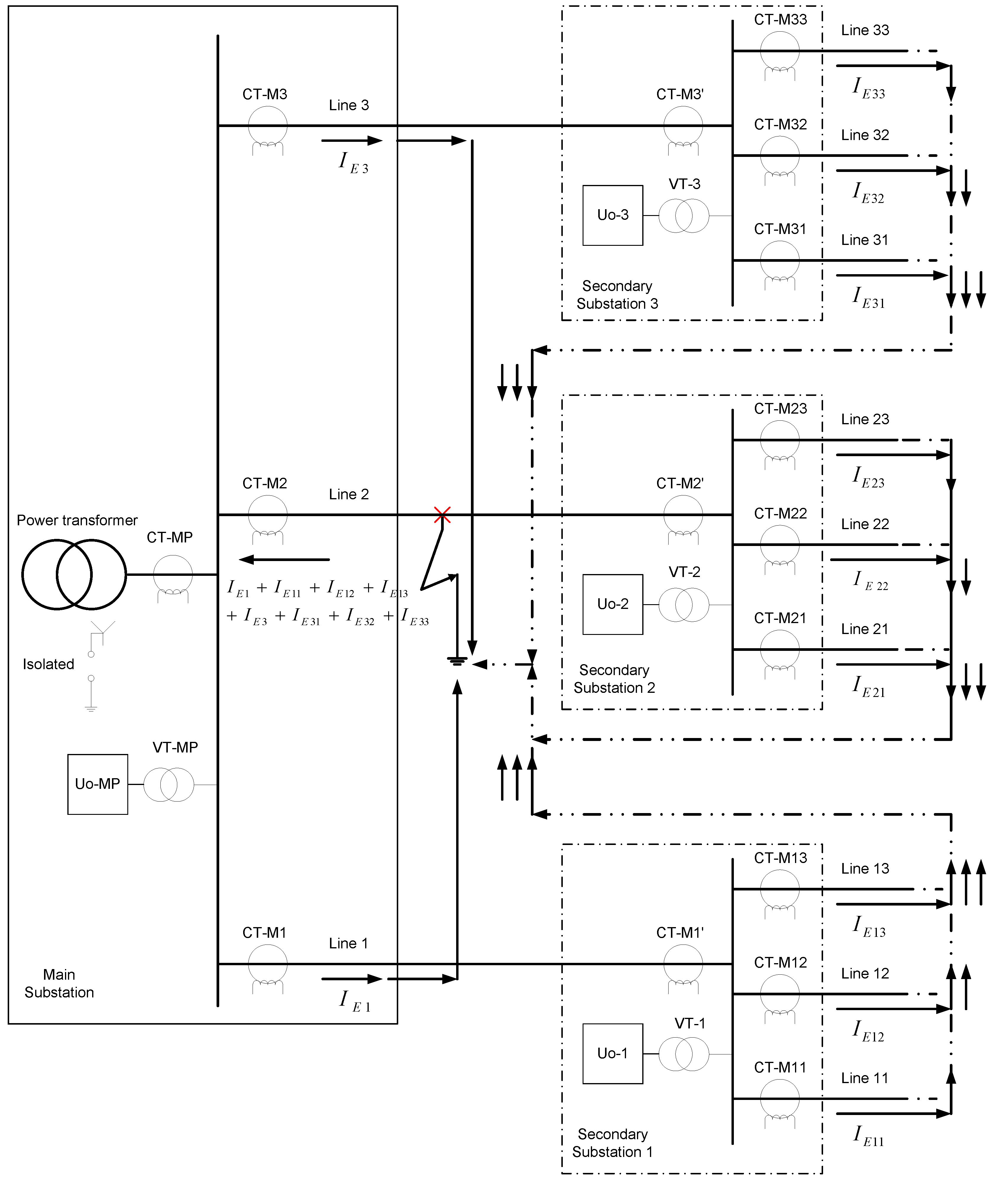
3.3.2. SPGF in a Line That Connects a Main Substation with a Secondary One

Now the network study is represented in Figure 10, where a ground fault has occurred in Line 2.

In this case, the new selective ground fault method operates as follows:

-

Residual voltage level is over the setting value, so the residual currents are evaluated.

-

At secondary substation 1, the defect current measured at the incoming Line 1 by its current transformer CT-M1’ has an rms value equal to the sum of the rms values of the defect currents measured at the outgoing Lines 11, 12 and 13 by their respective current transformers CT-M11, CT-M12 and CT-M13. The fault is not located at any of these outgoing lines as a result of second condition criterion. The same conclusion can be reached for the secondary substation 2 and 3.

-

At the main substation, the defect current measured at the incoming line by CT-MP has a different rms value than the sum of the rms values of the defect currents measured at the outgoing Lines 1, 2 and 3 by their respective current transformers CT-M1, CT-M2 and CT.M3. The defect current measured at the outgoing Line 2 by CT-M2 has the highest rms value of all the outgoing lines. The new method would switch off Line 2 as the result of the first condition criteria.

The SPGF at outgoing Line 2 is cleared following the first criterion of maximum rms value, as well; there is no tripping command at any other secondary substation as a result of the evaluation of the second condition criterion. Table 2 shows the results of the current transformers placed at the main and secondary substations indicated in Figure 10. The same result is obtained when the SPGF is at Lines 1 and 3. Finally, application at busbars that couple different substations has also given excellent results, with its implementation also being suitable.

Figure 10. Highest SPGF currents at isolated network with main and secondary substations. Ground fault at Line 2.

Figure 10. Highest SPGF currents at isolated network with main and secondary substations. Ground fault at Line 2.

Table 2. Residual Current Measurements. SPGF at Line 2—Phase “a”—rms current value (A).

Main station		Secondary substation II
CT-MP	0	CT-M2’	IE2 + IE21 + IE22 + IE23
CT-M1	IE1 + IE11 + IE12 + IE13	CT-M21	IE21
CT-M2	IE1 + IE11 + IE12 + IE13 + IE3 + IE31 + IE32 + IE33	CT-M22	IE22
CT-M3	IE3 + IE31 + IE32 + IE33	CT-M23	IE23
Secondary substation I		Secondary substation III
CT-M1’	IE1 + IE11 + IE12 + IE13	CT-M3’	IE3 + IE31 + IE32 + IE33
CT-M11	IE11	CT-M31	IE31
CT-M12	IE12	CT-M32	IE32
CT-M13	IE13	CT-M33	IE33

Table 2. Residual Current Measurements. SPGF at Line 2—Phase “a”—rms current value (A).

Main station		Secondary substation II
CT-MP	0	CT-M2’	IE2 + IE21 + IE22 + IE23
CT-M1	IE1 + IE11 + IE12 + IE13	CT-M21	IE21
CT-M2	IE1 + IE11 + IE12 + IE13 + IE3 + IE31 + IE32 + IE33	CT-M22	IE22
CT-M3	IE3 + IE31 + IE32 + IE33	CT-M23	IE23
Secondary substation I		Secondary substation III
CT-M1’	IE1 + IE11 + IE12 + IE13	CT-M3’	IE3 + IE31 + IE32 + IE33
CT-M11	IE11	CT-M31	IE31
CT-M12	IE12	CT-M32	IE32
CT-M13	IE13	CT-M33	IE33

In Table 3 the main differences between the different protection methods used to detect and clear SPGF at neutral ungrounded networks are listed.

Table 3. Comparison of the main features of the protection methods used nowadays to detect and clear SPGF at neutral ungrounded networks.

Check list for commissioning	Protection method
	Residual voltage (ANSI 59N)	Ground fault directional overcurrent (ANSI 67N)	New method non directional
Check VT polarity	No	Yes	No
Check CT polarity	No	Yes	No
Check wiring polarity of VT’s to protection system	No	Yes	No
check wiring polarity of CT’s to protection system	No	Yes	No
Check tripping angle between I0 and U0	No	Yes	No
Selective tripping	No	Yes	Yes
Easy to set in operation	Yes	No	Yes
Cost of the protection system	Low	High	Low
Time to put the protection system into operation	Short	Long	Short
Primary injection needed to test its functionality	No	Yes	No

Table 3. Comparison of the main features of the protection methods used nowadays to detect and clear SPGF at neutral ungrounded networks.

Check list for commissioning	Protection method
	Residual voltage (ANSI 59N)	Ground fault directional overcurrent (ANSI 67N)	New method non directional
Check VT polarity	No	Yes	No
Check CT polarity	No	Yes	No
Check wiring polarity of VT’s to protection system	No	Yes	No
check wiring polarity of CT’s to protection system	No	Yes	No
Check tripping angle between I0 and U0	No	Yes	No
Selective tripping	No	Yes	Yes
Easy to set in operation	Yes	No	Yes
Cost of the protection system	Low	High	Low
Time to put the protection system into operation	Short	Long	Short
Primary injection needed to test its functionality	No	Yes	No

4. Analysis of Simulation Results

The proposed selective SPGF protection method was simulated using Alternative Transient Program (ATP) while post-processing was done using Matlab. An equivalent “pi” model for lines was used as well as power transformers rated 132/20 kV, 10 MVA, with YNd11 connection group. The simplest and simplified schematic with one incoming line with 50 km in length and three outgoing lines with equal lengths of 150 km without any load connected (a) and the same circuit with different loads (b) are shown in Figure 11.

The parameters of any equivalent “pi” feeder for conductor type LA56 with diameter Φ = 9.45 mm and delta disposition (D_ab = 4 m, D_ac = 2.3324 m, D_bc = 2.3324 m) are: R = 0.6136 Ω/km; X = 0.4148 Ω/km and C = 0.28 μF/km. Loads: Z1 = 960 + j719.42 Ω; Z2 = 545 + j263.89 Ω; Z3 = 380 + j124.72 Ω.

Figure 11. ATP single line diagram for main substation arrangement.

Figure 11. ATP single line diagram for main substation arrangement.

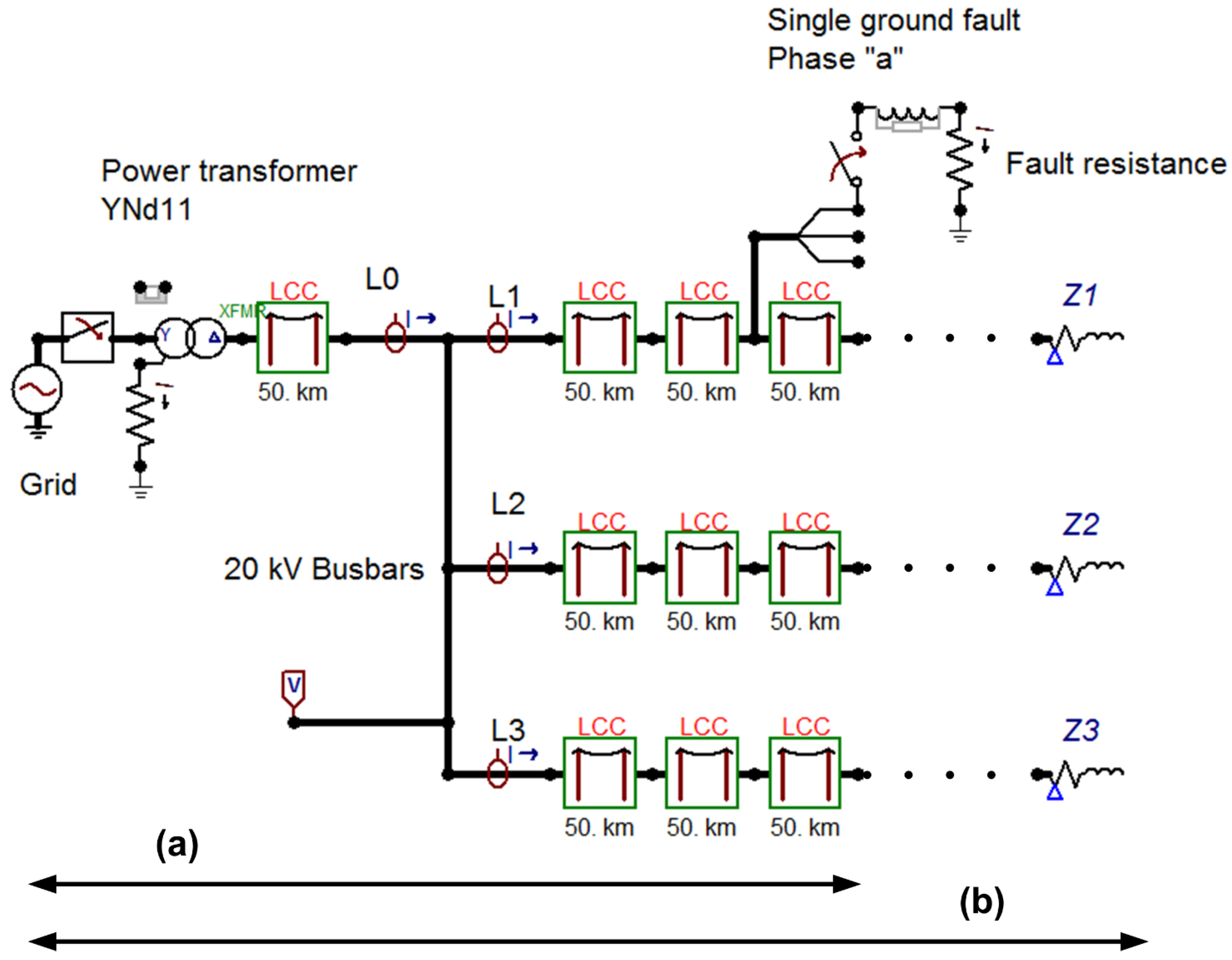
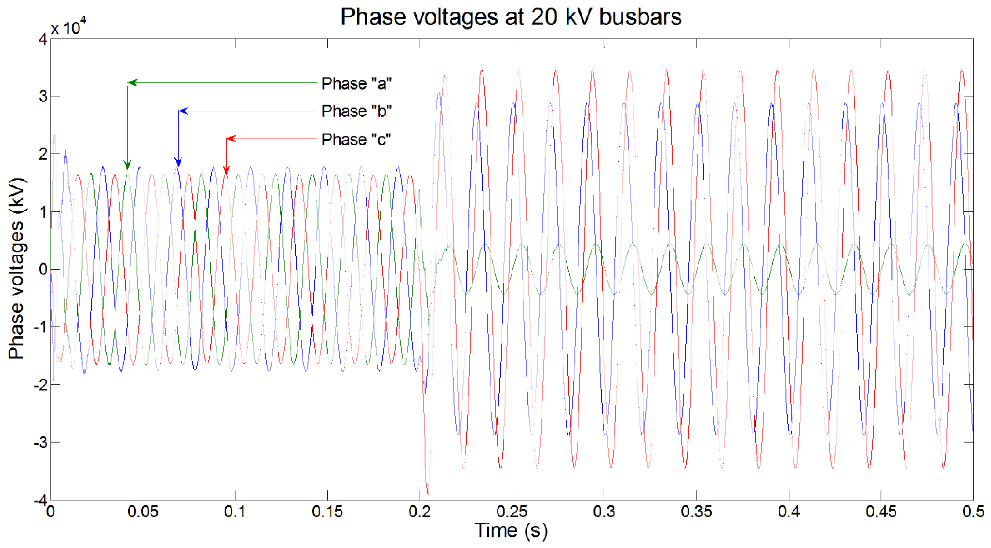
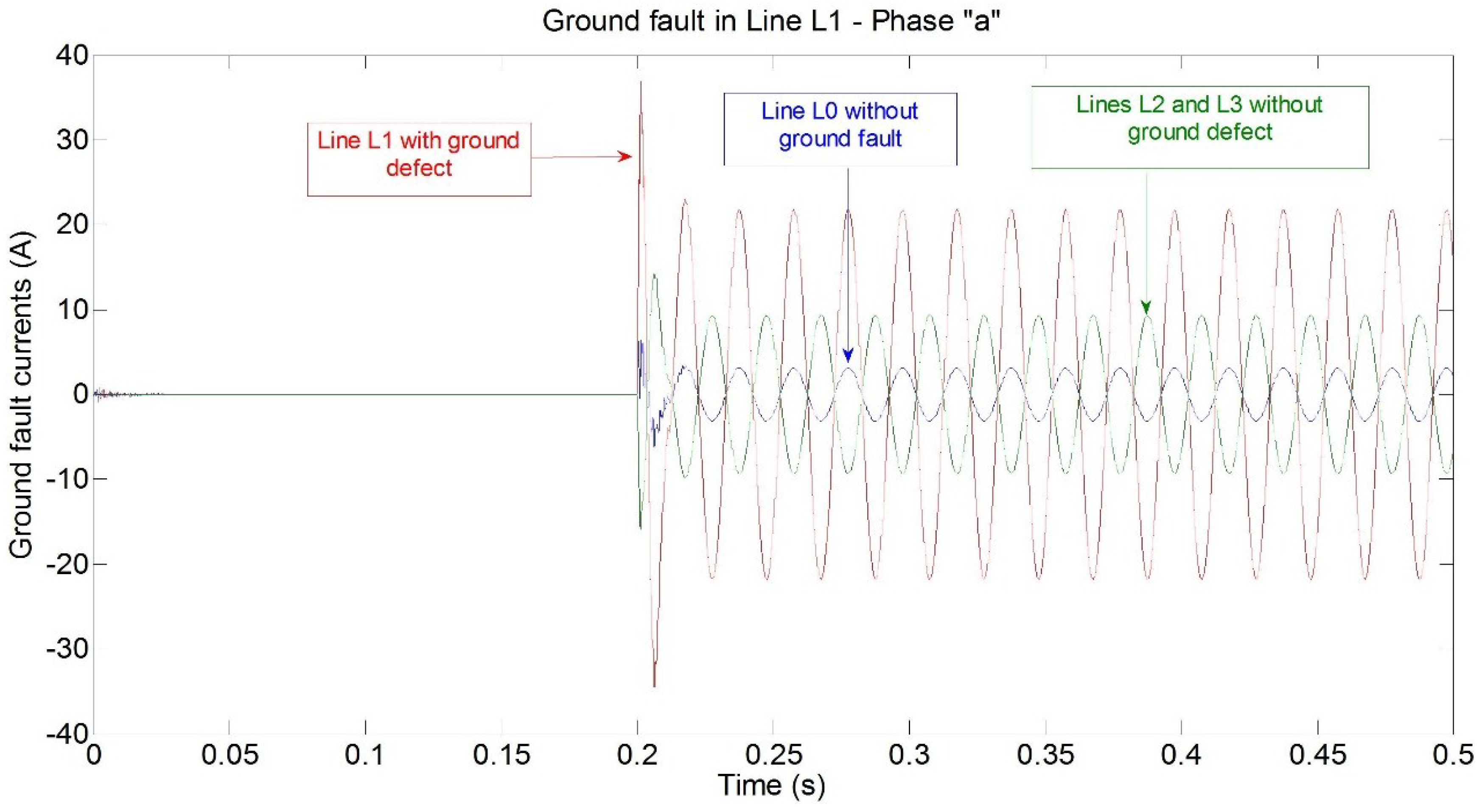
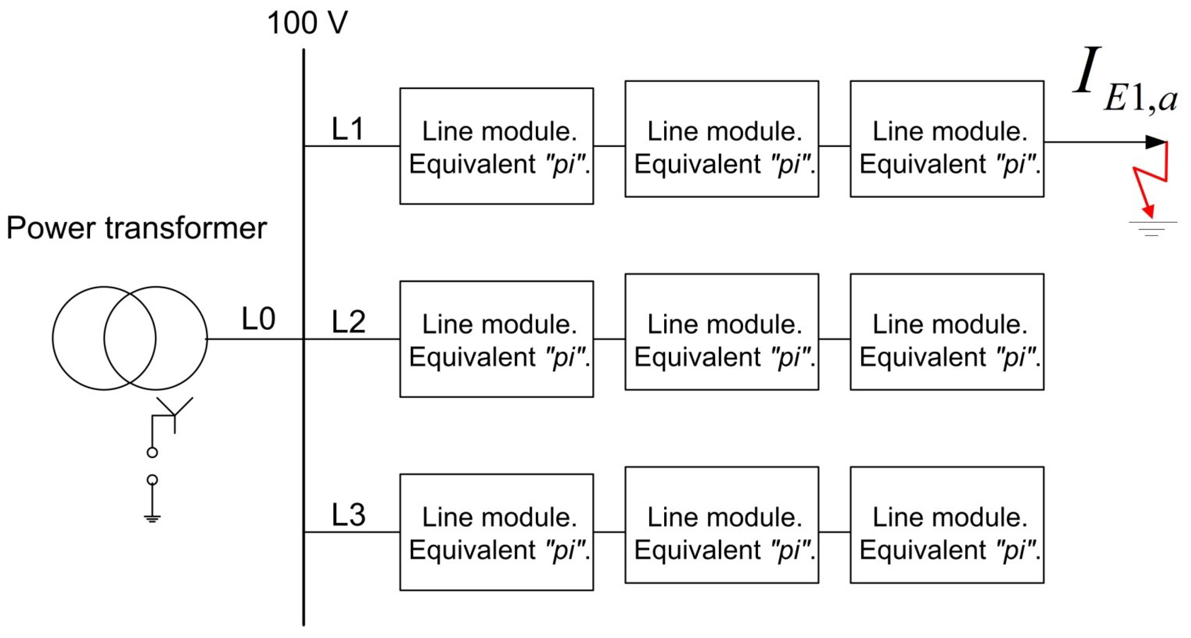
4.1. Main Substation

To simulate the new method for the detection of which line suffers a ground fault condition, a power system formed by three outgoing lines, of identical lengths, has been used, as seen in Figure 6. Simulations with load (a) and without load (b) at each line terminal have been carried out. In the simulation, ground faults were simulated at different phases and at different places with different resistance values up to 30 Ω. For instance, a ground fault at single line diagram shown in Figure 11 is evaluated at Line 1 phase “a” under no load conditions. Voltages under such fault condition at the distribution 20 kV busbars are shown in Figure 12. Voltages at the same distribution 20 kV busbars under the same fault conditions as before, but with load in the three feeders, turned out to be not so high—between 8 and 10 kV less. In Figure 13, all SPGF currents of all lines connected to the 20 kV busbars are represented considering the network as indicated in Figure 11 with load (b). The simulation results shown in Figure 13 are indicated in Table 4. It can be clearly observed that the line with the defect is the one which has the greatest residual current, its value being the sum of the other residual currents (I_E1 = I_E2 + I_E3 + I_E0). It is totally correct to say that using this proposed method in a main substation, a ground fault can easily be detected in a selective way.

Figure 12. Phase voltages at main distribution busbars. SPGF at phase “a”—Line 1.

Figure 12. Phase voltages at main distribution busbars. SPGF at phase “a”—Line 1.

Figure 13. Ground fault currents at main distribution busbars. SPGF at phase “a”—Line 1.

Figure 13. Ground fault currents at main distribution busbars. SPGF at phase “a”—Line 1.

Table 4. Residual current measurements. SPGF at Line 1—Phase “a”—rms current value (A).

Main station
	IE0	IE1	IE2	IE3
(a)	3.71	25.81	11.05	11.05
(b)	3.10	21.78	9.34	9.34

Table 4. Residual current measurements. SPGF at Line 1—Phase “a”—rms current value (A).

Main station
	IE0	IE1	IE2	IE3
(a)	3.71	25.81	11.05	11.05
(b)	3.10	21.78	9.34	9.34

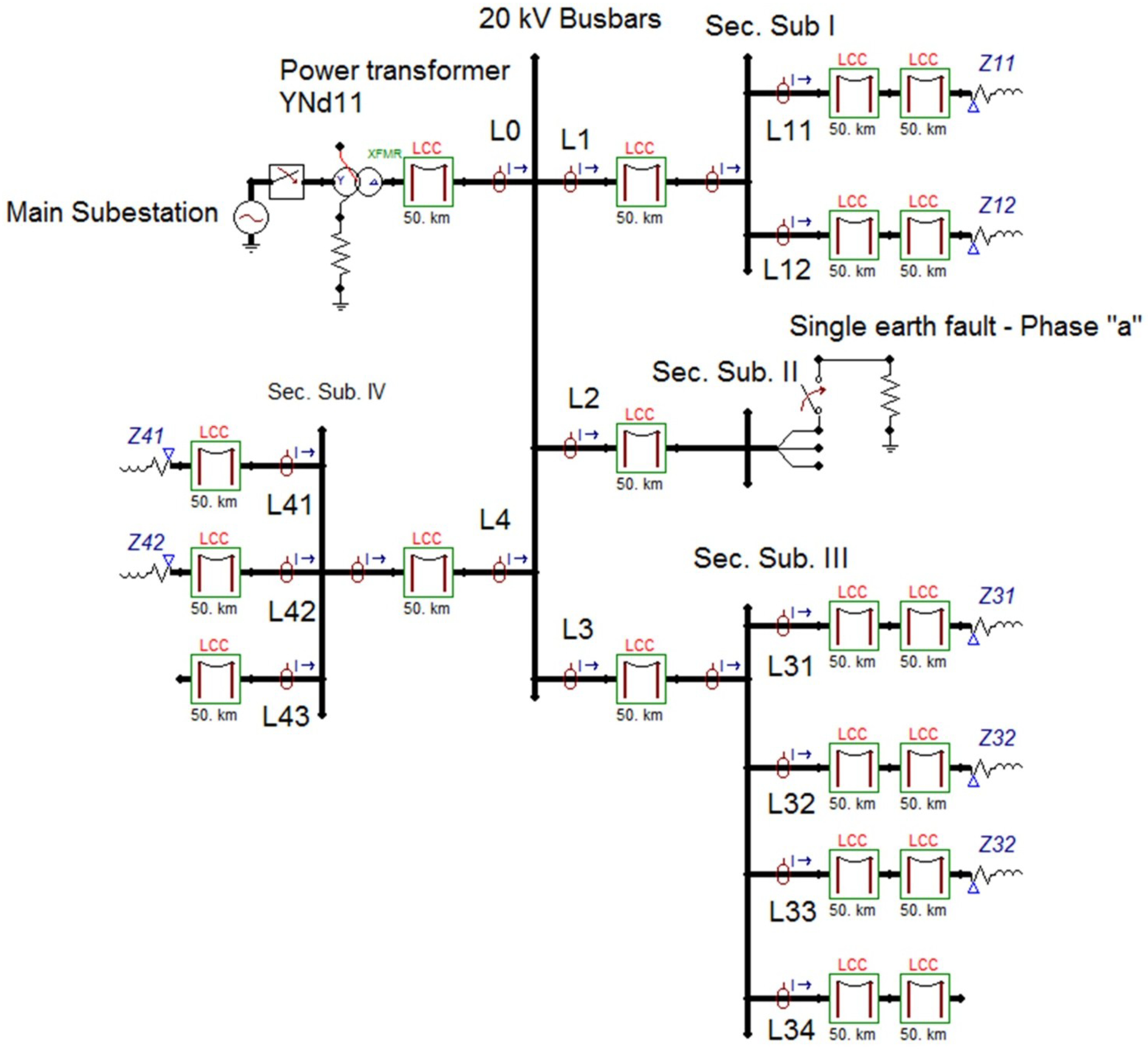
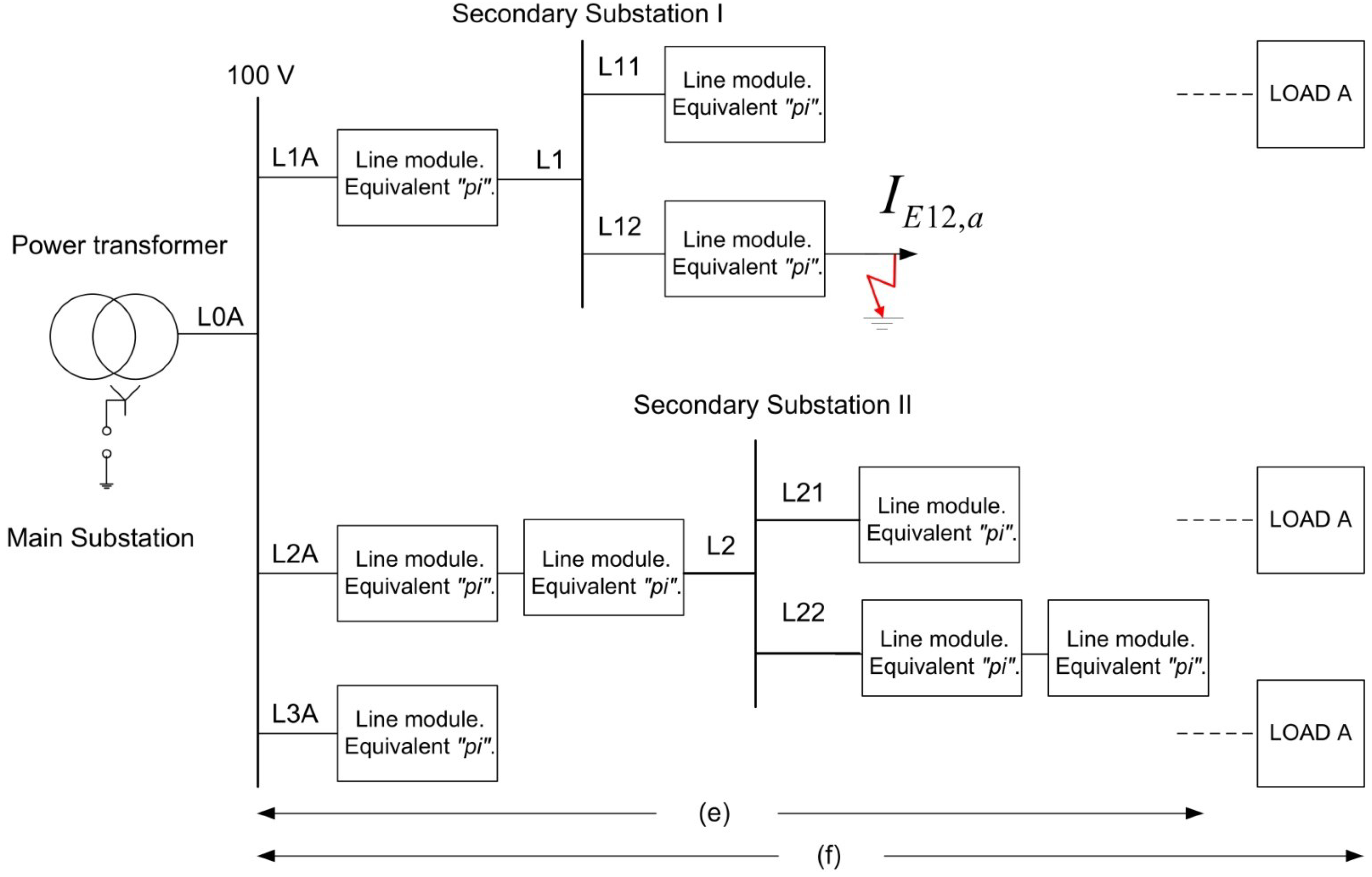
4.2. Secondary Substations

Figure 14 shows a network with one main substation and four secondary substations. Feeders L11, L12, L31, L32, L33, L41 and L42 supply different loads while feeders L2, L34 and L43 are energized without any load connected. Ground fault at Line 2 in phase “a” is evaluated, and the result shows that ground fault current measurements at 20 kV busbars verify the proposed method. Ground fault currents at outgoing Lines1, 3 and 4 with no fault, keep the same phase angle, whereas the ground fault current at the Line 2 with ground defect has a 180° phase angle difference compared to those of Lines1, 3 and 4 (Figure 15). The sum of the rms ground fault current values of Lines 0, 1, 3 and 4 is practically the same as that in Line 2.

Figure 14. Single line diagram for main and secondary substations.

Figure 14. Single line diagram for main and secondary substations.

Figure 15. Ground fault currents at main distribution busbars. Single ground fault at phase “a”—Line 2.

Figure 15. Ground fault currents at main distribution busbars. Single ground fault at phase “a”—Line 2.

On the other hand, the evaluation of the defect currents at the three secondary substations has shown that the incoming defect current rms value has the same defect current value as has the sum of the rms defect current values of all the outgoing lines, at each of the three secondary substations. Therefore, no tripping command will be given at any other secondary substation. Evaluation of the highest defect current rms value at the main substation will give a tripping order to the Line 2 switchgear where the ground fault is taking place. These results are listed in Table 5. In Figure 15, the ground fault currents of all lines connected to the 20 kV busbars are represented.

Table 5. Residual current measurements. SPGF at Line 2—Phase “a”—rms current value (A).

Main station
IE0	IE1	IE2	IE3	IE4
1.25	6.44	24.80	11.92	5.19
Secondary substation I
IE1	IE11		IE12
5.17	2.58		2.59
Secondary substation II
IE2		IE2
24.80		24.80
Secondary substation III
IE30	IE31	IE32	IE33	IE34
10.63	2.66	2.67	2.67	2.65
Secondary Substation IV
IE4	IE41	IE42	IE43
3.92	1.31	1.31	1.31

Table 5. Residual current measurements. SPGF at Line 2—Phase “a”—rms current value (A).

Main station
IE0	IE1	IE2	IE3	IE4
1.25	6.44	24.80	11.92	5.19
Secondary substation I
IE1	IE11		IE12
5.17	2.58		2.59
Secondary substation II
IE2		IE2
24.80		24.80
Secondary substation III
IE30	IE31	IE32	IE33	IE34
10.63	2.66	2.67	2.67	2.65
Secondary Substation IV
IE4	IE41	IE42	IE43
3.92	1.31	1.31	1.31

5. Experimental Results

To test the validity of the proposed SPGF detection method and its computer simulation results, different laboratory tests have been performed on an isolated network. These tests try to verify the operating principle of the detection technique.

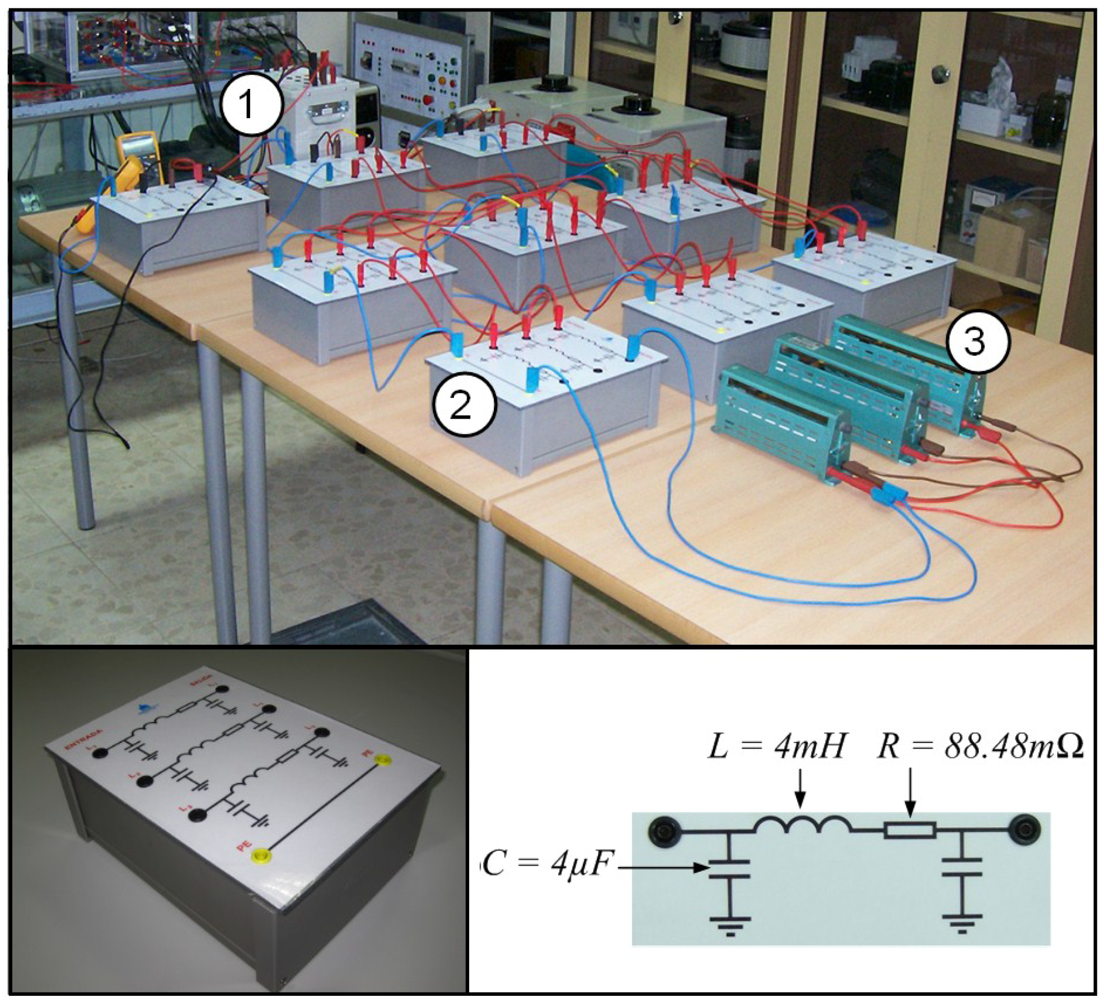
5.1. Experimental Setup

The tests were carried out on an isolated network supplied by a power transformer rated 800 VA, 400/100 Vac, and YNy0 connection group. Up to nine line modules with equivalent circuit “pi” were used, as shown in Figure 16. A per unit system of S_B = 800 VA, U_B = 100 V, I_B = 4.618 A, and Z_B = 12.5 Ω was selected to represent all values. These practical tests were carried out with loads and no loads at the end of the lines. The parameters of any equivalent “pi” feeder, also shown in Figure 16, have the following characteristics: R = 88.48 mΩ, L = 4 mH, and C = 4 μF each capacitor.

Figure 16. Top: Actual network experiment set-up. Three identical lines. (1: Power transformer, 2: Equivalent “pi” module, 3: Ground fault resistance). Bottom: Equivalent “pi” module and parameter values.

Figure 16. Top: Actual network experiment set-up. Three identical lines. (1: Power transformer, 2: Equivalent “pi” module, 3: Ground fault resistance). Bottom: Equivalent “pi” module and parameter values.

Several SPGFs at different phases, lines, and configurations were implemented in the real isolated network erected in the laboratory. The ground fault resistance was shifted from 0 to 2.4 p.u. in all cases studied.

5.2. Three Lines with Identical Lengths

This kind of single line network scheme is shown in Figure 17, where the lines have a total equivalent length of 150 km. Without any load connected (c), the measurements taken when a single ground fault is present at Line 1 are listed in Table 6, including the fault resistance R_f and the residual voltage U₀ measured at the busbars. The results show that the defect current measured at Line 1 has the highest value, compared to those registered at Lines 2 and 3. As shown in Table 6, the faults can be clearly located with different fault resistance values, chosen at random. The results obtained when having loads (d) as 300 VA in Line 1, 50 VA in Line 2 and 150 VA in Line 3 are listed in Table 7. Again, the results show that the defect current measured at Line 1 has the highest value, compared to those registered at Lines 2 and 3.

Figure 17. Single line diagram with three lines with equal length. SPGF at phase “a”—Line 1.

Figure 17. Single line diagram with three lines with equal length. SPGF at phase “a”—Line 1.

Table 6. Experimental results. Three lines not loaded with identical length. Residual current measurements I_E in per unit values (p.u.). SPGF at Line 1—Phase “a”.

Main station
Rf	U0	L1	L2	L3	IE1,a
0.00	1.38	0.80	0.40	0.40	1.18
0.32	1.21	0.70	0.35	0.35	1.03
0.56	1.19	0.73	0.34	0.34	0.97
0.80	1.03	0.59	0.30	0.30	0.88
1.04	0.82	0.47	0.24	0.24	0.70
1.20	0.75	0.47	0.23	0.23	0.69
1.60	0.62	0.36	0.18	0.18	0.53
2.00	0.53	0.30	0.15	0.15	0.45
2.40	0.47	0.26	0.13	0.13	0.39

Table 6. Experimental results. Three lines not loaded with identical length. Residual current measurements I_E in per unit values (p.u.). SPGF at Line 1—Phase “a”.

Main station
Rf	U0	L1	L2	L3	IE1,a
0.00	1.38	0.80	0.40	0.40	1.18
0.32	1.21	0.70	0.35	0.35	1.03
0.56	1.19	0.73	0.34	0.34	0.97
0.80	1.03	0.59	0.30	0.30	0.88
1.04	0.82	0.47	0.24	0.24	0.70
1.20	0.75	0.47	0.23	0.23	0.69
1.60	0.62	0.36	0.18	0.18	0.53
2.00	0.53	0.30	0.15	0.15	0.45
2.40	0.47	0.26	0.13	0.13	0.39

Table 7. Experimental results. Three lines loaded with identical length. Residual current measurements I_E in per unit values (p.u.). SPGF at Line 1—Phase “a”.

Main station
Rf	U0	L1	L2	L3	IE1,a
0.00	1.38	0.78	0.39	0.39	1.16
0.32	1.21	0.73	0.36	0.36	1.08
0.56	1.19	0.64	0.32	0.32	0.95
0.80	1.03	0.57	0.28	0.28	0.84
1.04	0.82	0.50	0.25	0.25	0.74
1.20	0.75	0.45	0.22	0.22	0.66
1.60	0.62	0.36	0.18	0.18	0.53
2.00	0.53	0.31	0.15	0.15	0.45
2.40	0.47	0.27	0.13	0.13	0.40

Table 7. Experimental results. Three lines loaded with identical length. Residual current measurements I_E in per unit values (p.u.). SPGF at Line 1—Phase “a”.

Main station
Rf	U0	L1	L2	L3	IE1,a
0.00	1.38	0.78	0.39	0.39	1.16
0.32	1.21	0.73	0.36	0.36	1.08
0.56	1.19	0.64	0.32	0.32	0.95
0.80	1.03	0.57	0.28	0.28	0.84
1.04	0.82	0.50	0.25	0.25	0.74
1.20	0.75	0.45	0.22	0.22	0.66
1.60	0.62	0.36	0.18	0.18	0.53
2.00	0.53	0.31	0.15	0.15	0.45
2.40	0.47	0.27	0.13	0.13	0.40

Figure 18. Multiple line network. SPGF at Line 12.

Figure 18. Multiple line network. SPGF at Line 12.

5.3. Three Different Line Lengths

This network is formed by three lines with different lengths of 150, 250, and 50 km. This kind of network with a SPGF at Line 12 is shown at Figure 18. Without any load connected (e), the measurements taken at Line 1 when a SPGF is present at Line 12 are listed in Table 8, where the fault resistance R_f and residual voltage U₀ measured at the main station are also included. The results show that the defect current measured at Line1A has the highest value, compared to those registered at Lines 2A and 3A. On the other hand, at Secondary Substation II, the incoming defect current at Line 2 is equal to the sum of the defect currents at outgoing Lines 21 and 22. Also in Figure 18, with different loads connected (f) in Lines 11, 21 and 3, the measurements taken when a SPGF is present at Lines 12 are listed in Table 9, where the fault resistance R_f and residual voltage U₀ measured at the main station are also included. Table 10 shows the defect currents at substations I and II as well as the defect current. The results again show that the defect current measured at Line 1A has the highest value, compared to those registered at Lines 2A and 3A. On the other hand, at Secondary Substation II, the incoming defect current at Line 2 is equal to the sum of the defect currents at outgoing Lines 21 and 22.

Table 8. Experimental results. Three lines not loaded with different lengths. Residual current measurements I_E in per unit values (p.u.). SPGF at Line 12—Phase “a”.

Main station						Secondary substation II
Rf	U0	L1A	L2A	L3A	IE12,a	L2	L21	L22
0.00	0.72	0.73	0.61	0.12	1.08	0.37	0.25	0.12
0.32	0.66	0.71	0.59	0.11	1.04	0.34	0.23	0.11
0.55	0.61	0.68	0.56	0.11	1.00	0.31	0.21	0.10
0.80	0.51	0.58	0.49	0.10	0.87	0.27	0.18	0.09
1.04	0.48	0.49	0.38	0.07	0.68	0.25	0.17	0.08
1.20	0.40	0.45	0.37	0.07	0.66	0.21	0.14	0.07
1.60	0.33	0.36	0.30	0.06	0.53	0.17	0.12	0.05
2.00	0.28	0.30	0.25	0.05	0.44	0.14	0.10	0.04
2.40	0.24	0.27	0.23	0.02	0.39	0.12	0.08	0.04

Table 8. Experimental results. Three lines not loaded with different lengths. Residual current measurements I_E in per unit values (p.u.). SPGF at Line 12—Phase “a”.

Main station						Secondary substation II
Rf	U0	L1A	L2A	L3A	IE12,a	L2	L21	L22
0.00	0.72	0.73	0.61	0.12	1.08	0.37	0.25	0.12
0.32	0.66	0.71	0.59	0.11	1.04	0.34	0.23	0.11
0.55	0.61	0.68	0.56	0.11	1.00	0.31	0.21	0.10
0.80	0.51	0.58	0.49	0.10	0.87	0.27	0.18	0.09
1.04	0.48	0.49	0.38	0.07	0.68	0.25	0.17	0.08
1.20	0.40	0.45	0.37	0.07	0.66	0.21	0.14	0.07
1.60	0.33	0.36	0.30	0.06	0.53	0.17	0.12	0.05
2.00	0.28	0.30	0.25	0.05	0.44	0.14	0.10	0.04
2.40	0.24	0.27	0.23	0.02	0.39	0.12	0.08	0.04

Table 9. Experimental results. Lines with and without load with different lengths. Residual current measurements I_E in per unit values (p.u.). SPGF at Line 12—Phase “a”.

Main station
Rf	U0	L1A	L2A	L3A	L0A
0.00	0.91	3.27	2.76	0.53	0.0074
0.32	0.84	2.56	2.25	0.44	0.0081
0.55	0.79	2.34	2.01	0.38	0.0056
0.80	0.66	2.18	1.76	0.34	0.0028
1.04	0.59	2.11	1.43	0.29	0.0020
1.20	0.48	2.03	1.70	0.33	0.0021
1.60	0.37	1.63	1.37	0.27	0.0012
2.00	0.33	1.40	1.18	0.23	0.0017
2.40	0.27	1.22	1.02	0.20	0.0048

Table 9. Experimental results. Lines with and without load with different lengths. Residual current measurements I_E in per unit values (p.u.). SPGF at Line 12—Phase “a”.

Main station
Rf	U0	L1A	L2A	L3A	L0A
0.00	0.91	3.27	2.76	0.53	0.0074
0.32	0.84	2.56	2.25	0.44	0.0081
0.55	0.79	2.34	2.01	0.38	0.0056
0.80	0.66	2.18	1.76	0.34	0.0028
1.04	0.59	2.11	1.43	0.29	0.0020
1.20	0.48	2.03	1.70	0.33	0.0021
1.60	0.37	1.63	1.37	0.27	0.0012
2.00	0.33	1.40	1.18	0.23	0.0017
2.40	0.27	1.22	1.02	0.20	0.0048

In general terms, it must be said that the results obtained within these tests have turned out to be totally similar to the ATP simulations carried out. Again, different fault resistance values were tested with satisfactory results.

Table 10. Experimental results. Lines with and without load with different lengths. Residual current measurements I_E in per unit values (p.u.). SPGF at Line 12—Phase “a”.

Secondary substation I					Secondary substation II
Rf	L1	L11	L12	IE12,a	L2	L21	L22
0.00	3.68	0.52	4.32	4.85	1.66	0.55	1.12
0.32	3.04	0.39	3.36	3.70	1.38	0.41	0.96
0.55	2.73	0.35	3.02	3.46	1.21	0.37	0.83
0.80	2.47	0.28	2.75	3.18	1.09	0.36	0.73
1.04	2.11	0.30	2.42	2.92	1.06	0.32	0.73
1.20	2.01	0.32	2.68	2.79	1.03	0.34	0.67
1.60	1.90	0.26	2.16	2.42	0.83	0.27	0.55
2.00	1.62	0.22	1.81	2.06	0.71	0.24	0.46
2.40	1.41	0.19	1.60	1.78	0.61	0.21	0.40

Table 10. Experimental results. Lines with and without load with different lengths. Residual current measurements I_E in per unit values (p.u.). SPGF at Line 12—Phase “a”.

Secondary substation I					Secondary substation II
Rf	L1	L11	L12	IE12,a	L2	L21	L22
0.00	3.68	0.52	4.32	4.85	1.66	0.55	1.12
0.32	3.04	0.39	3.36	3.70	1.38	0.41	0.96
0.55	2.73	0.35	3.02	3.46	1.21	0.37	0.83
0.80	2.47	0.28	2.75	3.18	1.09	0.36	0.73
1.04	2.11	0.30	2.42	2.92	1.06	0.32	0.73
1.20	2.01	0.32	2.68	2.79	1.03	0.34	0.67
1.60	1.90	0.26	2.16	2.42	0.83	0.27	0.55
2.00	1.62	0.22	1.81	2.06	0.71	0.24	0.46
2.40	1.41	0.19	1.60	1.78	0.61	0.21	0.40

6. Conclusions

A new selective single phase ground fault technique for neutral undergrounded networks has been presented in this article. This new method is suitable for all kinds of main substations with at least three feeders and secondary substations. The proposed non-directional detection technique is based on the comparison of the rms value of the ground fault currents at each line position of each substation.

At main substations, the highest ground fault current module belongs to the line with the ground fault. At secondary substations, if the ground fault current at the incoming line of the main busbars has the same rms value as the arithmetic sum of all outgoing ground fault currents, the fault is not located at any of the outgoing lines connected to those busbars, provided that a minimum residual voltage over an established setting value is present.

ATP simulations with different substation configurations turned out to be totally satisfactory as well as the experimental results of the laboratory tests. All of them show that the localization of the single phase ground fault is easy to find, without any possible mistake, identifying the corresponding line as the “line with ground fault condition.”

This new protection technique has the following advantages, when compared to traditional directional ground fault protection devices:

• It is much easier to measure the values of the ground defect currents than evaluate the direction of the ground defect currents compared to the residual voltage.
• In substations that cannot be removed from service, primary injection tests are not able to be developed, and the correct operation of the directional ground fault protection relays is not secured, whereas this new method is able to be totally commissioned without primary injection tests and its good performance can be granted without removing the substation from service.
• Unintentional wrong tripping commands given by directional protection relays due to wrong CTs and VTs polarities connections are avoided, as directional criterion is not used.
• It reduces dramatically the time and costs of installation and commissioning compared to the use of directional ground fault protection relays.

The aforementioned advantages provide a great improvement in the network protection system as unintended trips caused by single ground faults are eliminated.

References

1. L’Abbate, A.; Fulli, G.; Starr, F.; Peteves, S. Distributed power generation in Europe: Technical issues for further integration. JRC European Commission Scientific and Technical Report. EUR 23234 EN. 2007. [Google Scholar]
2. Russell Mason, C. The Art and Science of Protective Relaying; Wiley: New York, NY, USA, 1956; (sixth enlarged edition, 1967). [Google Scholar]
3. Horowitz, S.H.; Phadke, A.G. Power System Relaying; 3rd ed.; Wiley: New York, NY, USA, 2008. [Google Scholar]
4. Huang, S.J.; Wan, H.H. A Method to enhance ground-fault computation. IEEE Power Eng. Lett. IEEE Trans. Power Syst. 2010, 25, 1190–1191. [Google Scholar] [CrossRef]
5. Lin, W.M.; Ou, T.C. Unbalanced distribution network fault analysis with hybrid compensation. IET Gener. Transmiss. Distrib. 2011, 5, 92–100. [Google Scholar] [CrossRef]
6. Ou, T.C. A novel unsymmetrical faults analysis for microgrid distribution systems. Int. J. Electr. Power Energy Syst. 2012, 43, 1017–1024. [Google Scholar] [CrossRef]
7. Ou, T.C. Ground fault current analysis with a direct building algorithm for microgrid distribution. Int. J. Electr. Power Energy Syst. 2013, 53, 867–875. [Google Scholar] [CrossRef]
8. Lin, X.; Ke, S.; Gao, Y.; Wang, B.; Liu, P. A selective single phase-to-ground fault protection for neutral uneffectively grounded systems. IJEPES 2011, 33, 1012–1017. [Google Scholar]
9. Henriksen, T. Faulty feeder identification in high impedance grounded network using charge-voltage relationship. Electr. Power Syst. Res. 2011, 81, 1832–1839. [Google Scholar] [CrossRef]
10. Tamo, T.; Voufo, J. Fault diagnosis on medium voltage (MV) electric power distribution networks: The case of the downstream network of the AES-SONEL Ngousso sub-station. Energies 2009, 2, 243–257. [Google Scholar] [CrossRef]
11. Conti, S.; Nicotra, S. Procedures for fault location and isolation to solve protection selectivity problems in MV distribution networks with dispersed generation. Electr. Power Syst. Res. 2009, 79, 57–64. [Google Scholar] [CrossRef]
12. Saha, M.M.; Izykowsky, J.; Rosolowsky, E. Fault Location on Power Networks; Springer-Verlag: Berlin, Germany, 2009. [Google Scholar]
13. Granizo, R.; Blánquez, F.R.; Rebollo, E.; Platero, C.A. New selective earth faults only current directional method for isolated neutral systems. In Proceedings of the Environment and Electrical Engineering (EEEIC), Venice, Italy, 18–25 May 2012; pp. 18–25.
14. Chen, L.; Yang, Q.; Wang, J.; Sima, W.; Yuan, T. Classification of fundamental ferroresonance, single phase-to-ground and wire breakage over-voltages in isolated neutral networks. Energies 2011, 4, 1301–1320. [Google Scholar] [CrossRef]
15. Magnano, F.H.; Bur, A. Fault location using Wavelets. IEEE Trans. Power Deliv. 1998, 13, 1475–1480. [Google Scholar] [CrossRef]
16. Huang, J.; Hu, X.; Li, X.; Hu, H.; Lv, Y. A novel single-phase earth fault feeder detection by traveling wave and wavelets. In Proceedings of the International Conference on Power System Technology, Chongqing, China, 22–26 October 2006; pp. 22–26.
17. Elkalashy, N.; Lehtonen, M.; Darwish, H.; Taalab, A.M.; Izzularab, M. Operation evaluation of DWT-based earth fault detection in unearthed MV networks. In Proceedings of the MEPCON International Middle-East Power System Conference, Aswan, Egypt, 12–15 March 2008; pp. 208–212.
18. Xyngi, I.; Popov, M. Smart protection in Dutch medium voltage distributed generation systems. In Proceedings of the IEEE PES Innovative Smart Grid Technologies Conference Europe (ISGT Europe), Gothenburg, Sweden, 11–13 October 2010; pp. 1–8.
19. Ukil, A.; Deck, B.; Shah, V. Smart distribution protection using current-only directional overcurrent relay. In Proceedings of the IEEE PES Innovative Smart Grid Technologies Conference Europe (ISGT Europe), Gothenburg, Sweden, 11–13 October 2010; pp. 1–7.
20. Stojanovic, A.N.; Djuric, M.B. An algorithm for directional earth-fault relay with no voltage inputs. Electr. Power Syst. Res. 2013, 96, 144–149. [Google Scholar] [CrossRef]
21. Universidad Politécnica de Madrid. System and method for selective non-directional earth-fault protection in isolated neutral networks. Spanish Patent No. 2374345, 11 February 2013.