Article

Harmonic Injection-Based Power Fluctuation Control of Three-Phase PV Systems under Unbalanced Grid Voltage Conditions

1
State Key Laboratory of Power Transmission Equipment & System Security and New Technology, Chongqing University, Chongqing 400044, China
2
Department of Electrical Engineering and Computer Science, University of Wisconsin-Milwaukee, Milwaukee, WI 53211, USA
*
Author to whom correspondence should be addressed.
Energies 2015, 8(2), 1390-1405; https://doi.org/10.3390/en8021390
Submission received: 7 November 2014 / Accepted: 5 January 2015 / Published: 11 February 2015

Abstract

:
Unbalanced voltage will inevitably cause power and DC voltage fluctuations in a three-phase PV system. The deterioration of power quality will do great harm to the PV panels and the loads, so it is necessary to suppress the power fluctuations. This paper further explores the coefficients control strategy of PV converters under unbalanced voltage conditions, aiming to suppress power fluctuations by controlling the injection of some specific orders of current harmonics into the grid. In order to achieve this, the current reference of the PV inverter has been changed by bringing in two control coefficients, and the expression of each order of the current harmonics has been deduced. Based on the standards of PV systems, the regions from which the coefficients can be selected are determined. Then, by tuning these coefficients in the feasible regions, the output parameters (power fluctuation, current THD and odd harmonics) can be controlled precisely. The model of this method is built and simulated in PSCAD/EMTDC, and as a result, it is shown that the power fluctuations can be restricted according to different power quality requirements.

1. Introduction

Photovoltaic (PV) generation is widely used in renewable energy-penetrated DG systems for its easy installation [1,2,3,4]. The nonlinearity of power electronic devices and abnormal operation conditions such as grid harmonics and unbalanced voltage will lead to impacts on the power quality caused by PV systems [5,6,7]. Specifically, unbalanced voltage will inevitably cause power fluctuations in PV generation systems, which will lead to a voltage fluctuation on the DC side. Some research recommends bringing in current harmonics to suppress the power fluctuation. However, current harmonic pollution is restricted by the standards such as “Q/GDW617-2011” [8] and “IEEE Std. 1547™” [9]. Therefore, it is necessary to further study the operation characteristics of PV generation systems and the injected current harmonics to suppress power fluctuation under unbalanced voltage conditions.
The regulation strategy of positive and negative sequence currents under unbalanced voltage conditions is constructed in [10,11], and this method is designed to maintain a constant DC voltage. However, it ignores the influence on power quality caused by the current injection of the power converters. To make the converters meet the power quality requirements, five strategies are proposed to control the active and reactive power under unbalanced voltage, and they are used to tune the power fluctuation and current harmonic for specific purposes [12,13]. Accordingly, another control strategy, with which active and reactive power fluctuations are continuously adjustable, has been proposed in [14], but the current harmonics cannot be intuitively seen. The current instruction calculation method and the proportional multiple-integral current control strategy of PV under unbalanced voltage have been studied in [5], but the current reference is only designed to obtain a constant active power and unit power factor, which means the power fluctuation can be eliminated but at an expense of high current harmonic distortion [12]. Therefore, a novel control strategy has been proposed in [15,16]. In this method, the current reference is carefully revised by bringing in two coefficients α and β. Current THD, active and reactive power fluctuations of PV generation under unbalanced voltage conditions can be adjusted in a compromise by tuning these two coefficients. However, [15] only examines the THD of the output current. Actually, this method will bring in some low-order current harmonics, and the current THD is not the only indicator that should be suppressed. According to the grid-connected PV generation standards, the rate of each order of current harmonic in the output current should be specifically limited [8,9].
The novelty of this work is the suppression of the power fluctuation of a PV system under unbalanced faults by controlling the injection of specific orders of current harmonics. This work further explores the coefficients selection method in [15] by setting up feasible regions of the control coefficients so that these operational parameters (THD and each order of the harmonics) of the injected current can be limited within the required values. It starts with a discussion about the mechanism of power control and power fluctuation of PV generation under unbalanced grid voltage in Section 2. In Section 3, the analytic formulas of the root-mean-square (RMS) values of some basic low-order current harmonics are derived, and then the values of the current THD and each order of harmonic corresponding to the relevant adjustment coefficients group are analyzed. In Section 4, two control methods which are used to suppress the specific power fluctuation with the proper injected harmonic current under unbalanced voltage are designed. In the final part, the feasibility of the strategy is verified in PSCAD/EMTDC.

2. Control of PV Systems under Unbalanced Grid Voltage Conditions

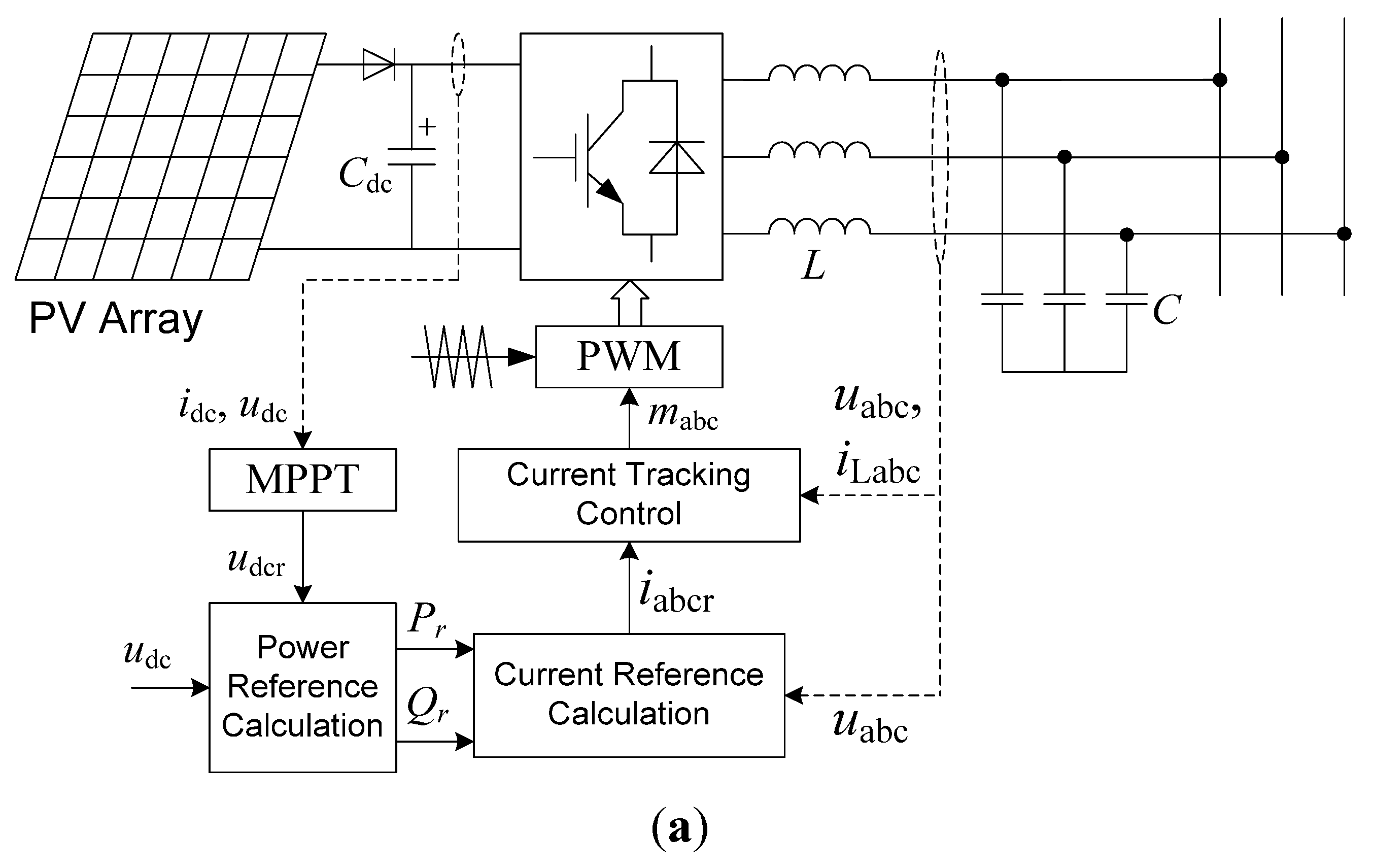
A three-phase single-stage PV system and its control diagram are shown in Figure 1, where the PV array works as a controlled current source model whose output power is varied with illumination intensity and the temperature [2,15]. In order to ensure the PV arrays works at the maximum power point, the voltage udc and current idc at DC side are collected. Then, the DC voltage generated from the maximum power point tracking (MPPT) module is taken for the dc voltage reference udc, and the power instruction Pr and Qr can be hereby obtained. At the same time, the current and voltage information at the grid side is gathered. Combining them with the power instructions, then the reference current iabcr can be calculated. Power control of the grid-connected photovoltaic system can be realized through the current tracking control link.
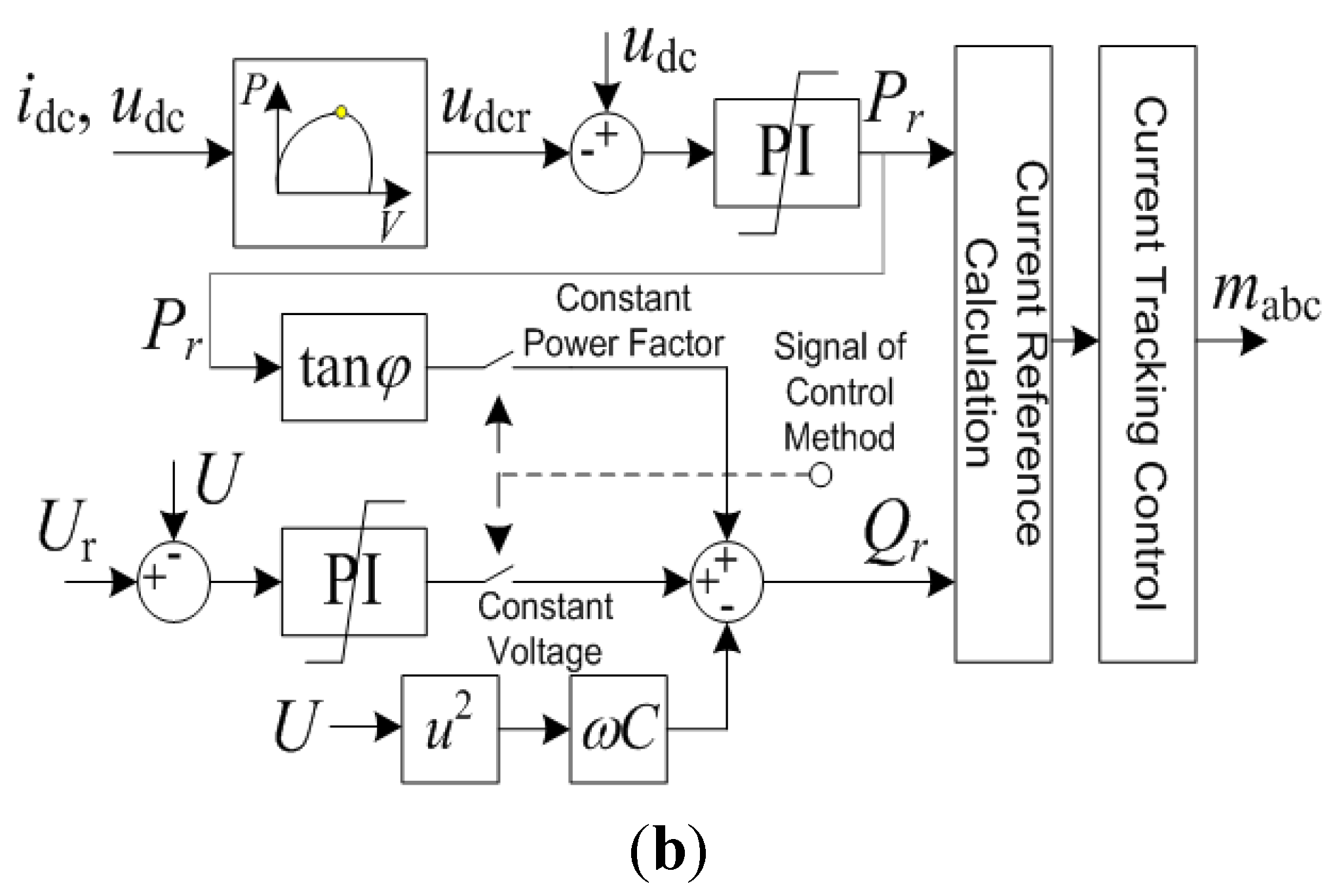
The model in Figure 1b has applied increment conductance method to produce the voltage reference udcr at the maximum power point [17]. Then the active power reference Pr can be obtained by comparing the actual DC voltage udc with the reference value udcr. There are two reactive power control methods: constant power factor control and constant voltage control. As to the constant power factor control, the reactive power reference can be calculated with the power factor (PF) cosφ and the active power reference Pr. And as to the constant voltage control, the reactive power reference can be obtained by the deviation of the actual voltage U and the voltage reference Ur through the proportional integrator (PI) controller. In the control system in Figure 1b, since the inductor current feedback is used in the current tracking module, the reactive power reference Qr can be obtained after the reactive power of the filter capacitor is subtracted. There is a lot of research on the maximum power tracking of PV systems [17,18], but this paper mainly focuses on the current reference calculation and the power fluctuation suppression of PV systems under unbalanced voltage conditions.
Figure 1. Grid-connected photovoltaic system: (a) The structure of PV generation system and (b) Power control of PV system.
Energies 08 01390 g001aEnergies 08 01390 g001b
A power distribution network is usually neutral un-grounded or Petersen-coil grounded, and there is no zero-sequence current. Hence, under unbalanced grid voltage conditions, the output voltage of a PV system will contain positive, negative and zero sequence components, while the current will only contain positive and negative components. The output current and voltage of the PV system can be represented in vector format:
i ( t ) = i + ( t ) + i ( t ) = [ i a + ( t ) , i b + ( t ) , i c + ( t ) ] T + [ i a ( t ) , i b ( t ) , i c ( t ) ] T u ( t ) = u + ( t ) + u ( t ) + u 0 ( t ) = [ u a + ( t ) , u b + ( t ) , u c + ( t ) ] T + [ u a ( t ) , u b ( t ) , u c ( t ) ] T + [ u a 0 ( t ) , u b 0 ( t ) , u c 0 ( t ) ] T
where u+(t), u(t) and i+(t), i(t) are respectively the positive and negative sequence components of the output voltage and current, and u0(t) is the zero-sequence voltage component. The three-phase instantaneous active power can be expressed as the dot product of the voltage vector and the current vector:
p ( t ) = u ( t ) i ( t ) = u + ( t ) i + ( t ) + u ( t ) i ( t ) + u + ( t ) i ( t ) + u ( t ) i + ( t ) p ˜ ( t )
The instantaneous reactive power is the module value of the cross product of u(t) and i(t) [12]. Due to symmetry of the components in u+(t) and u(t), the dot products between u0(t) and positive-sequence or negative-sequence current vectors are also always zero [14], which means there’s no need to calculate the zero-sequence voltage component without a zero-sequence current component. In order to simplify the calculation, we can build a new vector u(t) which is orthogonal to u(t):
u ( t ) = u + ( t ) + u ( t )    = [ u b + ( t ) u c + ( t ) , u c + ( t ) u a + ( t ) , u a + ( t ) u b + ( t ) ] T / 3    + [ u b ( t ) u c ( t ) , u c ( t ) u a ( t ) , u a ( t ) u b ( t ) ] T / 3
The zero-sequence component of the orthogonal voltage vector u(t) is u0(t) = 0, so u(t) is only combined with positive and negative components. The three phase instantaneous reactive power can be expressed as:
q ( t ) = | u ( t ) × i ( t ) | = u ( t ) i ( t )   = u + ( t ) i + ( t ) + u ( t ) i ( t ) + u + ( t ) i ( t ) + u ( t ) i + ( t ) q ˜ ( t )
When the PV is under unbalanced grid voltage conditions, the positive and negative components of voltage and current will rotate reversely, which will lead to a double-frequency fluctuation in the instantaneous active and reactive powers, that can be expressed as p ˜ ( t ) and q ˜ ( t ) . According to Equation (3), the values of u(t) and u(t) are equal, and |u+(t) + u(t)|2 = |u+(t) + u(t)|2. In order to stabilize the active and reactive powers under unbalanced voltage, the output current should be controlled. The current reference can be derived from Equations (2) and (4) as:
i r ( t ) = P r [ u + ( t ) + u ( t ) ] | u + ( t ) + u ( t ) | 2 + Q r [ u + ( t ) + u ( t ) ] | u + ( t ) + u ( t ) | 2    = P r [ u + ( t ) + u ( t ) ] + Q r [ u + ( t ) + u ( t ) ] | u + ( t ) | 2 + 2 u + ( t ) u ( t ) + | u ( t ) | 2
If the current reference in formula Equation (5) is applied to control the PV system, the output power can track the power references Pr and Qr accurately and the output power fluctuation can be eliminated, but at the expense of a large amount of harmonics in the output current. Hence it is necessary to slightly modify the current reference by bringing in two accommodation coefficients α and β to realize a flexible control towards the power fluctuation by injecting some current harmonics [15]. According to [15], the current reference with coefficients above can be modified as:
i r ( t ) = P r [ u + ( t ) + α u ( t ) ] + Q r [ u + ( t ) + α u ( t ) ] | u + ( t ) | 2 + ( 1 + α ) β u + ( t ) u ( t ) + α | u ( t ) | 2
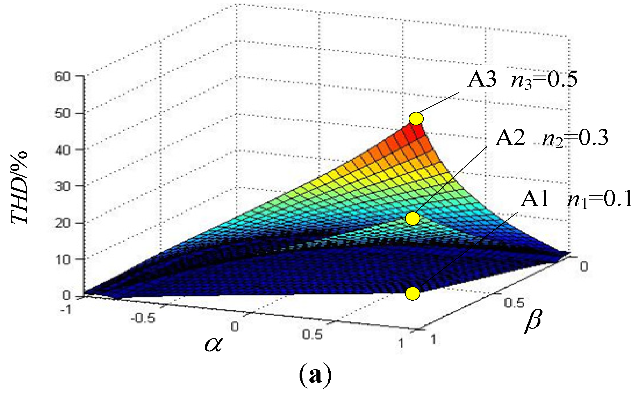
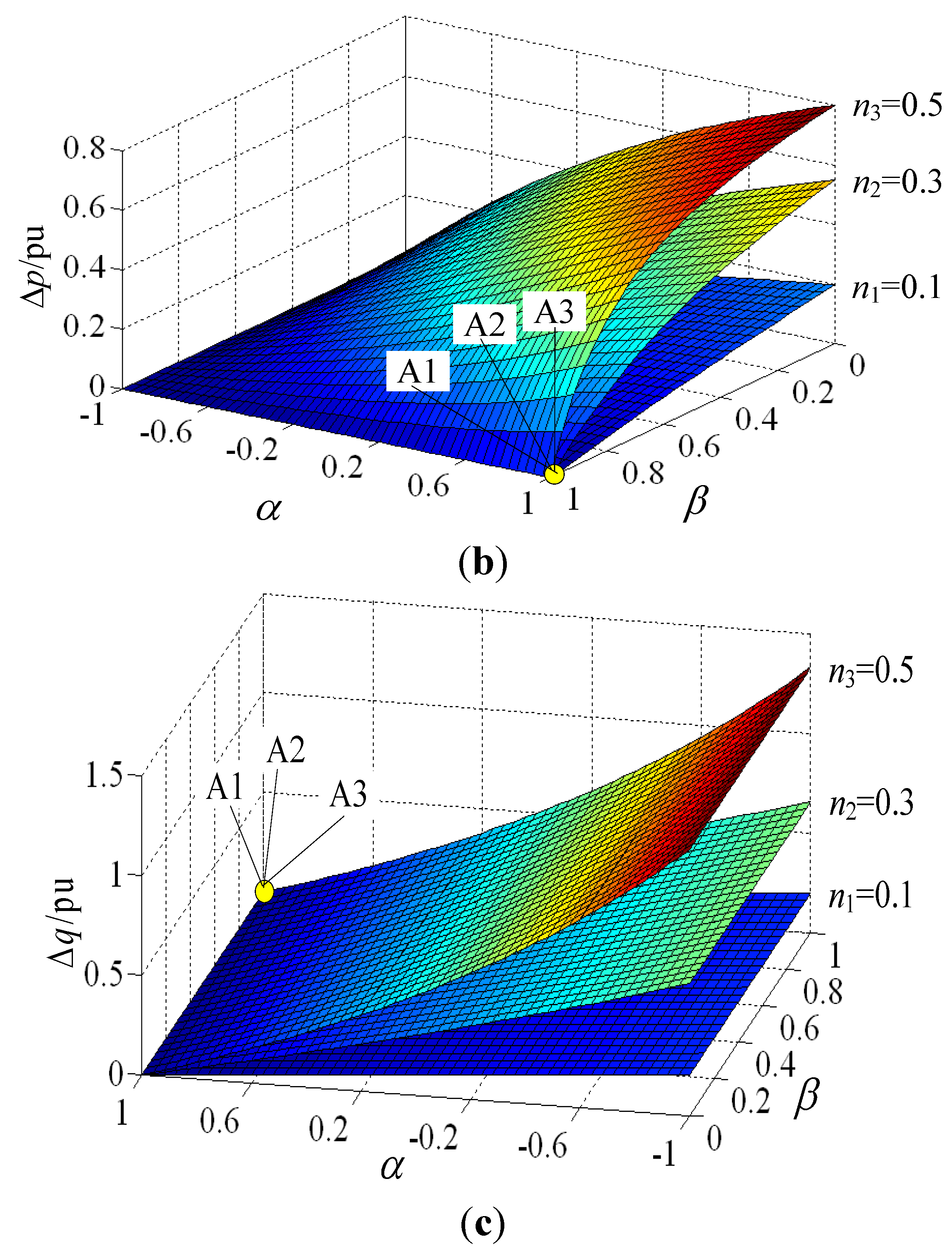
where we set α∈ [–1,1] and β∈ [0,1] (α rising from −1 to 1 means the injection of more harmonics into the grid to suppress the reactive power fluctuation. α = −1 ensures the current to be sinusoidal and α = 1 ensures the active power fluctuation to be eliminated; β rising from 0 to 1 means injecting more harmonics to suppress the active power fluctuation. β = 0 ensures the output current to be sinusoidal. β = 1 ensures the active power fluctuation to be zero). Adjusting the coefficients α and β properly can suppress the magnitudes of active and reactive fluctuations by injecting a small amount of current harmonics which should also meet the standards.

3. Characteristic Analysis and Calculation of the Harmonics Current of PV Generation under Unbalanced Grid Voltage Conditions

3.1. Analysis of Current THD and Power Fluctuation

According to the technical requirements of PV systems, the power factor should be larger than 0.9 (no matter whether leading or lagging) under grid-connected mode conditions [9]. Hence the reactive power reference should be set to be zero, that is Qr = 0. The PV systems are connected to the distribution network and they are required to serve lots of unbalanced loads which will lead to a serious voltage imbalance in a long period. As discussed in Section 2, there is no need to calculate the zero-sequence component in the output voltage in the neutral ungrounded grid. Thus, the voltage imbalance can be characterised as the ratio of the positive and negative sequence components: n = U/U+, defined as the unbalanced voltage factor. The three-phase current expression in time domain can be derived from Equation (6), and the current of phase a is:
i ra ( t ) = 2 P r 3 U + ( 1 + α n ) cos ( ω t ) 1 + β ( 1 + α ) n cos ( 2 ω t ) + α n 2
From Equation (7), we can get the RMS values of the fundamental and the whole frequency waves of the PV current, which are I1 and I. Then the current THD can be expressed as follows [15]:
T H D = I 2 I 1 2 1 = 1 T 0 T [ i ra ( t ) ] 2 d t [ 2 T 0 T i ra ( t ) cos ( ω t ) d t ] 2 1 = A 2 2 C ( B C ) 1
where A = β (1 + α)n, B = 1 + αn2 and C = B 2 A 2 . Combining Equations (2), (4) and (7), we can obtain the amplitudes of active and reactive power fluctuations as Equations (9) and (10). The power fluctuations can be adjusted as the coefficients are changed:
Δ p = [ p ˜ ( t ) p ( t ) - p ˜ ( t ) ] max = ( 1 β ) ( 1 + α ) n 1 β ( 1 + α ) n + α n 2
Δ q = [ q ˜ ( t ) p ( t ) - p ˜ ( t ) ] max = ( 1 α ) n 1 + α n 2
As shown in Figure 2, under each of the three different situations where the unbalanced voltage factors are n = 0.1, 0.3, 0.5, the changing trends of the parameters (current THD, the active and the reactive power fluctuations) with the variation of the coefficients α and β can be presented in three-dimensional diagrams according to Equations (8) to (10).
A1, A2 and A3 are the three operation points where the coefficients are selected as (α, β) = (1, 1) under different unbalanced voltages (n1, n2, and n3 relatively). The three operation points in the above figures present the occasions before α and β are brought in: active and reactive power fluctuations are eliminated at an expense of injecting high current harmonics. The figures have shown that the more we restrain the fluctuation of the PV system, the more current harmonics must be injected into the grid.
Figure 2. Three-dimensional meshes of current total harmonic distortion and power fluctuation magnitudes: (a) Current THD; (b) Active Power Fluctuation and (c) Reactive Power Fluctuation.
Energies 08 01390 g002aEnergies 08 01390 g002b
The figure also demonstrates that the active power fluctuation can be restrained by decreasing α or increasing β, and the reactive power can be restrained by increasing α. In addition, decreasing α and β at the same time can reduce the THD of the output current. Hence, the current adjustment coefficients should be selected reasonably under unbalanced voltage conditions in order to satisfy the restraints of the output current harmonics.

3.2. Odd Harmonics Calculation and Analysis

According to the IEEE Std 1547™ for grid-connected PV systems under steady state conditions, besides the THD injected into the grid is limited below 5%, each order of the harmonics is also limited respectively. In [9,15] the PV coefficients are selected only by considering the current THD. The method in [15] overlooks some specific order of harmonics that will still go out of limits even though THD is within its limit, which will not meet the requirement of the standard for grid-connected PV systems. In order to find the area where the coefficients should be chosen, it is necessary to calculate the RMS value of the kth order harmonic current Ik:
I k = 1 2 [ 2 T 0 T i ra ( t ) sin ( k ω t ) d t ] 2 + [ 2 T 0 T i ra ( t ) cos ( k ω t ) d t ] 2 = d e f 1 2 E k 2 + F k 2
From Equation (11), we can know that the even orders of current harmonics are cancelled out so that they are negligible (the calculation process is omitted here). The odd order harmonics will be mainly discussed in the paper. Substituting Equation (7) into (11) we can get the values of E3 and F3 of the third order current harmonics of the PV system under unbalanced voltage as:
E 3 = 2 T 0 T i ra ( t ) sin ( 3 ω t ) d t = 2 P r ( 1 + α n ) 3 U + T ( 0 T sin ( 4 ω t ) + sin ( 2 ω t ) 1 + β ( 1 + α ) n cos ( 2 ω t ) + α n 2 d t )
F 3 = 2 T 0 T i ra ( t ) cos ( 3 ω t ) d t = 2 2 P r ( 1 + α n ) 3 U + A 2 P r ( 1 + α n ) 3 U + T ( 2 B A + 1 ) 0 T 2[cos ( ω t ) ] 2 A cos ( 2 ω t ) + B d t 2 P r ( 1 + α n ) 3 U + [ 2 A 2 B / A + 1 C ( A + B ) ]
In Equation (12), the integral term E3 = 0 because it is an odd function in its period. Using numerical method, we can find that the term 2[cos(ωt)]2/[Acos(2ωt) + B] is approximately equal to T/[C(A + B)]1/2 in period T. Then we can get the RMS value of the third order current harmonic as:
I 3 = 1 2 E 3 2 + F 3 2 = P r ( 1 + α n ) 3 U + [ 2 B / A + 1 C ( A + B ) 2 A ]
In a similar way, the RMS values of the fifth and seventh order harmonics can be expressed as:
I 5 = P r ( 1 + α n ) 3 U + [ 4 B A 2 + 1 T ( 2 B A + 4 B 2 A 2 1 ) 0 T 2[cos ( ω t ) ] 2 A cos ( 2 ω t ) + B d t ] = P r ( 1 + α n ) 3 U + [ 4 B 2 / A 2 + 2 B / A 1 C ( A + B ) 4 B A 2 ]
I 7 = P r ( 1 + α n ) 3 U + [ 2 A + 8 B 2 A 3 + 1 T ( 8 B 3 A 3 + 4 B 2 A 2 4 B A 1 ) 0 T 2[cos ( ω t ) ] 2 A cos ( 2 ω t ) + B d t ] = P r ( 1 + α n ) 3 U + [ 8 B 3 / A 3 + 4 B 2 / A 2 4 B / A 1 C ( A + B ) + 2 A 8 B 2 A 3 ]
Set Pr = 1.0 pu, U+ = 1.0 pu and the unbalanced voltage of n = 0.3 will last for a relatively long period. Figure 3a shows the relationship among the current harmonics from 3rd to 9th and the varying coefficients α and β.
Figure 3. Current harmonics values: (a) Rms values of current harmonics from 3rd to 9th and (b) Calculation and simulation values of 3rd and 5th current harmonics.
Energies 08 01390 g003aEnergies 08 01390 g003b
Similar to the changing trend of the current distortion, RMS values of harmonics from 3rd to 9th will increase as the coefficients α and β increase. Figure 3b presents the simulation and calculation results of the 3rd and 5th current harmonics, which indicates that the calculation result derived in this paper matches the simulation result.
Under unbalanced voltage conditions, the higher order harmonics will have lower RMS values. In addition, based on the tendency, odd harmonics higher than 9th order are far below their limits so that there is no need to calculate them all.
In this paper, a case of a PV generation system with a rated voltage of 380 V and a rated capacity of 10 MVA is created. According to the Chinese standard Q/GDW617-2011 [8] for PV systems connected to the power grid, under steady state conditions, the output odd current harmonics from 3rd to 9th of the PV system in this case should be lower than 0.0041 pu, 0.0041 pu, 0.0029 pu and 0.0014 pu, respectively. Some international standards for PV systems, such as IEEE Standard 1547™ [9], specify that the current harmonics whose order is lower than 11th should be lower than 4%.
Figure 4 shows the contour lines where the values of the output current harmonics from 3rd to 9th and the THD are respectively equal to their specified limits based on different harmonics standards. The bottom left sides of the contour lines are the feasible regions, in which the harmonics can be limited, for α and β. From the figures, we can draw a conclusion that, based on the harmonic limits, the intersection of the regions determined by these current harmonics and THD is the region determined by the 3rd order current harmonic, so that the coefficients α and β should be selected based on the limit of the 3rd order current harmonic. The feasible region can be determined as Equation (17). I3lim can be the contour line of I3lim = 0.0041 pu in Figure 4a or I3lim = IL × 4% in Figure 4b based on different standards:
A ( I 3 ) = { ( α,β ) | P r ( 1 + α n ) 3 U + [ 2 B / A + 1 C ( A + B ) 2 A ] < I 3 lim , 1 < α < 1 , 0 < β < 1 }
Figure 4. The contour lines of odd current harmonics and current THD: (a) Feasible region based on “Q/GDW617-2011” and (b) Feasible region based on “IEEE Std. 1547™”.
Energies 08 01390 g004

4. Current Harmonics Injection Strategies of PV Systems under Unbalanced Grid Voltage Conditions with Different Control Objectives

Equation (6) can be used to realize power control of the PV system under unbalanced grid voltage conditions. As is shown in Table 1, the characteristics of the power fluctuation and the current harmonics can be determined when the coefficients α and β are set as different integers. We can see that the discrete variation of the coefficients α and β may make the PV system operate under extreme cases [12,13]. If the PV system is set to operate at a point which compromises power fluctuation and current harmonics, the coefficients α and β should be adjusted properly.
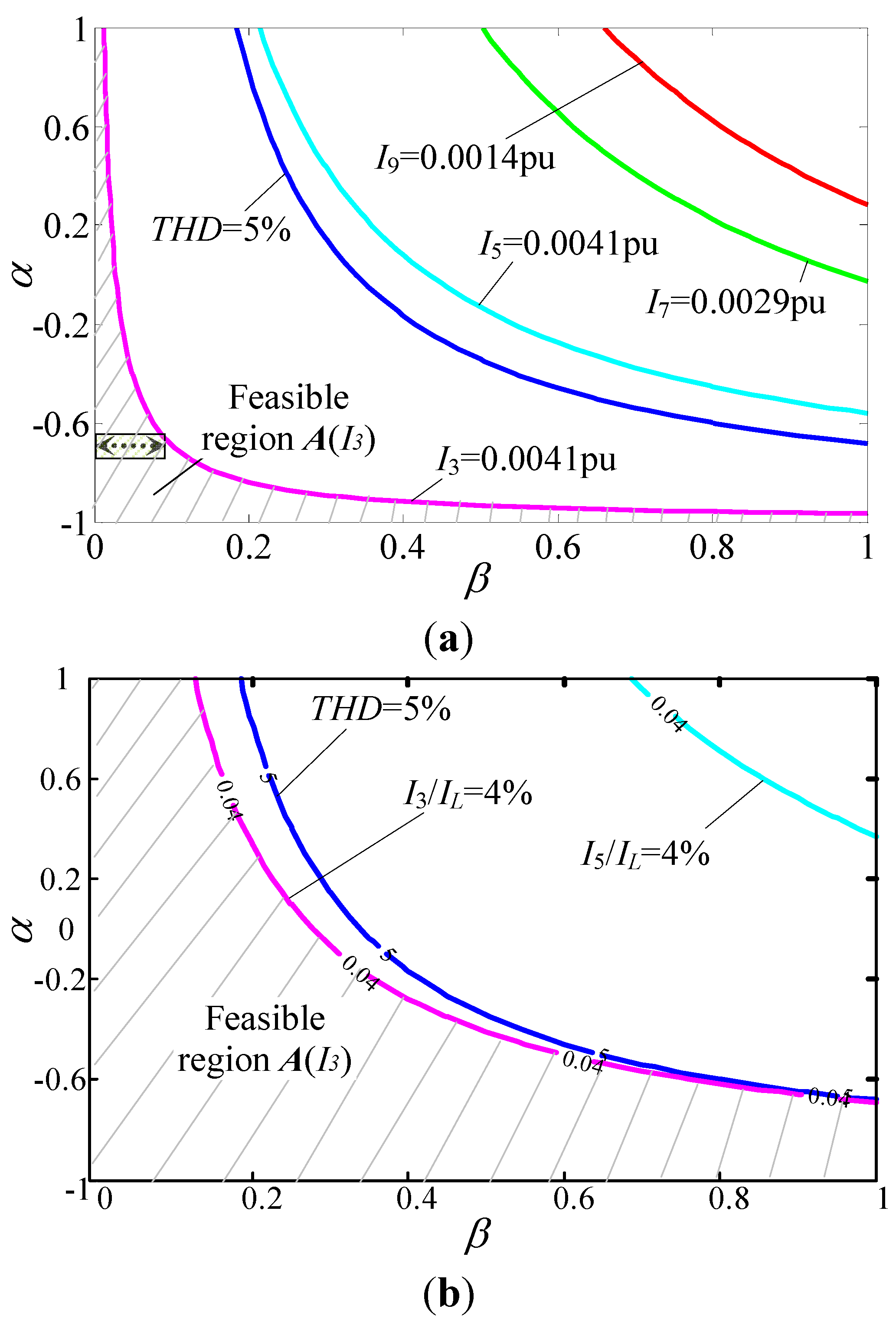
The current harmonic limit is an essential factor of PV systems even under unbalanced grid voltage conditions. Hence, we combine the third order current harmonic limit with the reactive and active power reference expressions, ΔQr and ΔPr. Two methods with specific objectives are designed as follows.
Table 1. Power fluctuation and 3rd harmonic current characteristic under different adjustment.
αβΔpΔqI3
1100 P r 3 U + n [ n 2 + n + 1 1 n 2 n 1 ]
10 2 n 1 + n 2 00
010n P r 3 U + [ 2 / n + 1 1 n 2 ( n + 1 ) 2 n ]
00nn0
−11 or 00 2 n 1 n 2 0

4.1. Method (a): Active Power Suppression within the Third Order Harmonics Limit

If the reactive power fluctuation is set under unbalanced voltage conditions, we can get the expression of coefficient α from Equation (10) as:
α = n Δ Q r n ( 1 + n Δ Q r )
Like the above expression, coefficient α can be determined by the unbalance factor n and ΔQr. From Equation (14), the equation where the third order current harmonic is expressed as I3r can be obtained:
[ 3 U + I 3r n ( α + 1 ) β + 2 P r ( α n + 1 ) ] [ ( α n 2 + 1 ) + n ( α + 1 ) β ] ( α n 2 + 1 ) 2 [ n ( α + 1 ) β ] 2 P r n ( α + 1 ) ( α n + 1 ) β 2 P r ( α n 2 + 1 ) ( α n + 1 ) = 0
Substituting Equation (18) into (19), we can get the equation of β. The equation can be solved by the Newton method (the analytic solution cannot be obtained). The numerical solution is the coefficient β which will satisfy the limit requirements of the reactive fluctuation and the third order current harmonic. As said in Section 2, we should choose the real number solution from β ∈ [0,1].

4.2. Method (b): Reactive Power Suppression within the Third Order Harmonics Limit

If the active power fluctuation of the PV system is set, the relationship between α and β can be obtained from Equation (9), as:
α = Δ P r ( 1 β n ) n ( 1 β ) n [ 1 β + Δ P r ( β n ) ]
Similarly, substituting the above expression into Equation (19), and the coefficient β which is applied to satisfy the limits of the active fluctuation and the third order current harmonic can be obtained with the Newton method. Then substituting β into Equation (20) we can get the corresponding coefficient α.
In a word, Equations (17) to (19) have turned α and β into intermediate variables, which makes the control method more straightforward. With method (a), ΔQr is set and increasing I3r will help to suppress ΔPr. On the other hand, with method (b), ΔPr is set and increasing I3r will help to suppress Δ
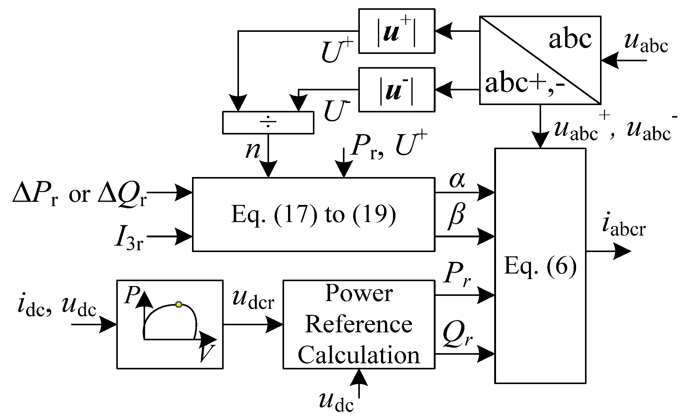
Qr. The block diagram of the proposed controller is shown in Figure 5.
Figure 5. Online adjustment of coefficients α and β for harmonic currents suppression.
Energies 08 01390 g005
In Figure 5, the positive- and negative-sequence voltage components uabc+ and uabc are extracted from the terminal of the PV system. According to the expressions from Equations (18) to (20), the coefficients α and β can be calculated with the given values of power fluctuation references ΔPr and ΔQr, the third order current limit I3r and the unbalance factor n. In addition, the dead-beat current control is used in the current tracking model, which is specifically stated in [12].

5. Simulation Analysis

The PV generation system is built in PSCAD/EMTDC with a rated capacity of 2.5 kVA, L = 12 mH, C = 0.7 μF, Cdc = 1800 μF, and the rated voltages on AC and DC sides are 220 V (RMS) and 1000 V, respectively. Firstly, we take α and β as the direct control variables. Assume that the PV system is serving an unbalanced voltage with n = 0.3, the calculation and the simulation results of the third and the fifth order of current harmonics under different coefficients α and β are shown in 
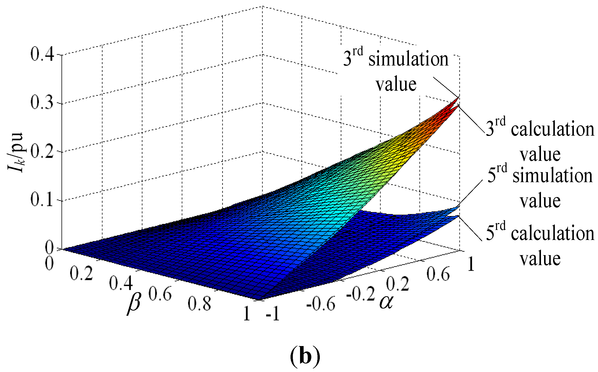
Table 2. Comparing these two groups of calculation results with each other, we can draw a conclusion that the analytical calculation results of the power fluctuation and the current harmonic derived before are basically consistent with the simulation results. The changing trends of these parameters (p, q, I3, I5) with coefficients α and β, are the same as what are shown in Figure 2, which means that this control method has a relatively high accuracy.
Table 2. Comparison between calculation and simulation results under different adjustment coefficient conditions.
Group No.αβMethodsΔp/puΔq/puI3/puI5/pu
10.51Calculation00.1310.2130.048
Simulation0.0240.1540.2340.054
20.50.5Calculation0.2740.1310.1090.012
Simulation0.2660.1470.1130.015
30.20.5Calculation0.2150.2260.0860.008
Simulation0.1970.2150.0910.012
40.20Calculation0.3540.22600
Simulation0.3170.2420.0090.007
Then the control model I and II are established based on the methods (a) and (b) in Section 4. Control model I is built to suppress the active power fluctuation, shown in Figure 6. An unbalanced voltage of n = 0.3 occurs at t = 0.5 s and the reactive power fluctuation reference is set to be ΔQr = 0.3 pu. Two situations of different third order current harmonic injection of I3r = 0.004 pu and I3r = 0.1 pu are shown in Figure 6a,b, and the coefficients (α, β) of these two coefficients are respectively generated as (0.012, 0.031) and (0.009, 0.657).
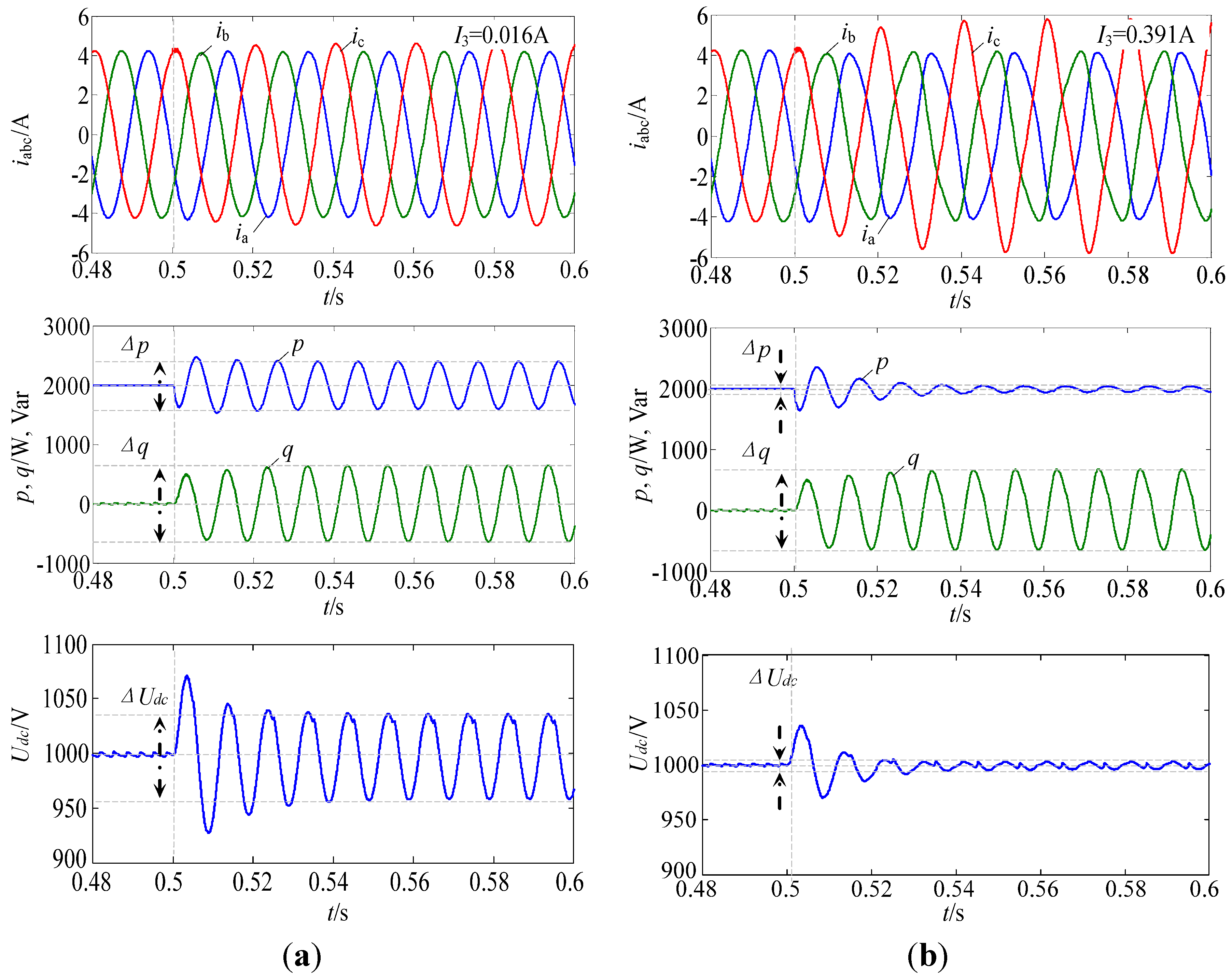
Figure 6. Operation characteristics of photovoltaic generation using control mode I: (a) I3r = 0.004 pu and ΔQr = 0.3 pu and (b) I3r = 0.1 pu and ΔQr = 0.3 pu.
Energies 08 01390 g006
As is shown in Figure 6a,b, the reactive power fluctuations are almost in the same value of 0.288 pu (tested in the simulation model), which is fixed to ΔQr (the reactive power fluctuation reference is set to be 0.3 pu). The active power fluctuations are 45% and 1% in Figure 6a,b respectively. The DC voltage fluctuation (ΔUDC/UDC) is 7% in Figure 6a and is 0.9% in Figure 6b. The simulation values of I3 are 0.004 pu and 0.103 pu respectively, which shows that the injected 3rd order harmonic current can track the set reference. As more 3rd order harmonic current is injected into the grid, the active power fluctuation and the DC voltage fluctuation can be suppressed to be lower. This control model can be applied to suppress the active power fluctuation and protect the PV array under unbalanced voltage.
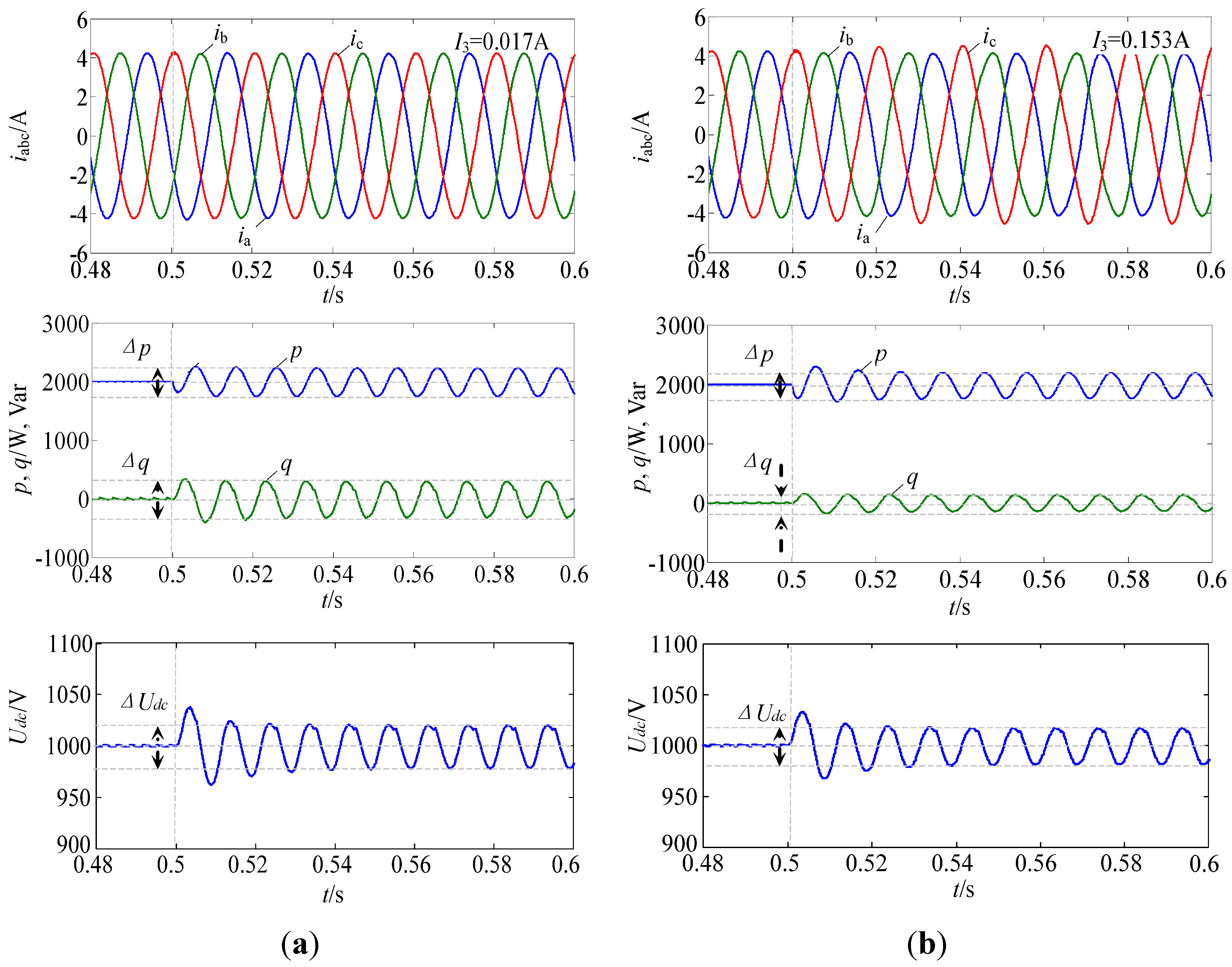
Control model II is built to suppress the reactive power fluctuation, shown in Figure 7. An unbalanced voltage of n = 0.3 occurs at t = 0.5 s and the active power fluctuation is set to be ΔPr = 0.1 pu. The third order harmonic injections are set as I3r = 0.004 pu or I3r = 0.04 pu in Figure 7a,b respectively. Due to the voltage synchronization module, a slight transient component will appear in the instantaneous power of PV system at the moment that an unbalanced voltage occurs [14]. After the transient response, as is shown in Figure 7a,b, the adjustment coefficients (α, β) would change to (−0.458, 0.124) and (−0.141, 0.475). As more amount of third order current harmonic current is injected into the grid, the output reactive power fluctuation will decrease. Control model II is helpless to suppress the DC voltage fluctuation. This model is mainly used to suppress the reactive power fluctuation, and it can be applied to ensure the stability of reactive power supply.
Figure 7. Operation characteristics of photovoltaic generation using control mode II: (a) I3r = 0.004 pu and ΔPr = 0.1 pu and (b) I3r = 0.04 pu and ΔPr = 0.1 pu.
Energies 08 01390 g007

6. Conclusions

This paper has expanded the coefficients selection control method to power fluctuation suppression under unbalanced voltage conditions by accurately injecting current harmonics into the grid. Adjusting the coefficients of the current control in the feasible regions continuously can realize a flexible control of power fluctuation and current harmonics, which highly enables the practical application of this method. This paper has obtained two calculation methods of the current adjustment coefficients: with the first method, the coefficients α and β are determined by the active power fluctuation and the 3rd order current harmonic limits; with the second one, the coefficients are determined by the reactive power fluctuation and the 3rd harmonic limits. In addition, through the simulation test of a PV system, the derived results of the power fluctuation and each order of the current harmonic match the simulation results well. As a result, by controlling the injection of harmonics into the grid, method I can suppress the active power fluctuation and the DC voltage fluctuation, while method II can effectively eliminate the reactive power fluctuation.

Acknowledgments

This work was supported by the National Natural Science Foundation of China (51277184), and National High Technology Research and Development of China (863 Program) (2011AA05A107).

Author Contributions

Nian-Cheng Zhou proposed the idea of harmonic injection control for PV system under unbalanced voltage; Xiao-Xuan Lou was in charge of the derivation of the equations and the feasible regions. He responded to the reviewers and revise the manuscript. David Yu checked the language and revise the contents of this manuscript. Qiang-Gang Wang built the simulation model. Jia-Jia Wang was responsible for the simulation data processing.

Conflicts of Interest

The authors declare no conflict of interest.

References

  1. Guerrero, J.M.; Blaabjerg, F.; Zhelev, T.; Hemmes, K.; Monmasson, E.; Jemei, S.; Comech, M.P.; Granadino, R.; Frau, J.I. Distributed Generation: Toward a New Energy Paradigm. IEEE Ind. Electron. Mag. 2010, 4, 52–64. [Google Scholar] [CrossRef]
  2. Baran, M.E.; Hooshyar, H.; Zhan, S.; Huang, A. Accommodating high pv penetration on distribution feeders. IEEE Trans. Smart Grid 2012, 3, 1039–1046. [Google Scholar] [CrossRef]
  3. Xiong, L.; Peng, W.; Poh Chiang, L. A hybrid AC/DC microgrid and its coordination control. IEEE Trans. Smart Grid 2011, 2, 278–286. [Google Scholar] [CrossRef]
  4. Papavasiliou, A.; Oren, S.S. Large-Scale Integration of deferrable demand and renewable energy sources. IEEE Trans. Power Syst. 2014, 29, 489–499. [Google Scholar] [CrossRef]
  5. Castilla, M.; Miret, J.; Camacho, A.; Matas, J.; Garcia de Vicuna, L. Voltage support control strategies for static synchronous compensators under unbalanced voltage sags. IEEE Trans. Ind. Electron. 2014, 61, 808–820. [Google Scholar] [CrossRef]
  6. Castilla, M.; Miret, J.; Camacho, A.; Matas, J.; de Vicuna, L.G. Reduction of current harmonic distortion in three-phase grid-connected photovoltaic inverters via resonant current control. IEEE Trans. Ind. Electron. 2013, 60, 1464–1472. [Google Scholar] [CrossRef] [Green Version]
  7. Xin, T.; Tsang, K.M.; Chan, W.L. A power quality compensator with DG interface capability using repetitive control. IEEE Trans. Energy Convers. 2012, 27, 213–219. [Google Scholar] [CrossRef]
  8. State Grid Corporation of China. Technical rule for Photovoltaic Power Station Connected to Power Grid; “Q/GDW617–2011”; State Grid Corporation of China: Beijing, China, 2011; pp. 15–18. [Google Scholar]
  9. The Institute of Electrical and Electronics Engineers. IEEE Standard for Interconnecting Distributed Resources with Electric Power Systems; IEEE Std 1547.2-2008; The Institute of Electrical and Electronics Engineers (IEEE): New York, NY, USA, 2008; pp. 9–10. [Google Scholar]
  10. Hong-Seok, S.; Kwanghee, N. Dual current control scheme for PWM converter under unbalanced input voltage conditions. IEEE Trans. Ind. Electron. 1999, 46, 953–959. [Google Scholar] [CrossRef]
  11. Yongsug, S.; Lipo, T.A. Control scheme in hybrid synchronous stationary frame for PWM AC/DC converter under generalized unbalanced operating conditions. IEEE Trans. Ind. Appl. 2006, 42, 825–835. [Google Scholar] [CrossRef]
  12. Rodriguez, P.; Timbus, A.V.; Teodorescu, R.; Liserre, M.; Blaabjerg, F. Flexible active power control of distributed power generation systems during grid faults. IEEE Trans. Ind. Electron. 2007, 54, 2583–2592. [Google Scholar] [CrossRef]
  13. Rodriguez, P.; Timbus, A.; Teodorescu, R.; Liserre, M.; Blaabjerg, F. Reactive power control for improving wind turbine system behavior under grid faults. IEEE Trans. Power Electron. 2009, 24, 1798–1801. [Google Scholar] [CrossRef]
  14. Fei, W.; Duarte, J.L.; Hendrix, M.A.M. Pliant active and reactive power control for grid-interactive converters under unbalanced voltage dips. IEEE Trans. Power Electron. 2011, 26, 1511–1521. [Google Scholar] [CrossRef]
  15. Castilla, M.; Miret, J.; Sosa, J.L.; Matas, J.; de Vicuña, L.G. Grid-fault control scheme for three-phase photovoltaic inverters with adjustable power quality characteristics. IEEE Trans. Power Electron. 2010, 25, 2930–2940. [Google Scholar] [CrossRef]
  16. Miret, J.; Castilla, M.; Camacho, A.; Garcia de Vicuna, L.; Matas, J. Control scheme for photovoltaic three-phase inverters to minimize peak currents during unbalanced grid-voltage sags. IEEE Trans. Power Electron. 2012, 27, 4262–4271. [Google Scholar] [CrossRef]
  17. Safari, A.; Mekhilef, S. Simulation and hardware implementation of incremental conductance MPPT with direct control method using cuk converter. IEEE Trans. Ind. Electron. 2011, 58, 1154–1161. [Google Scholar] [CrossRef]
  18. Guan-Chyun, H.; Hung, I.H.; Cheng-Yuan, T.; Chi-Hao, W. Photovoltaic power-increment-aided incremental-conductance MPPT with two-phased tracking. IEEE Trans. Power Electron. 2013, 28, 2895–2911. [Google Scholar] [CrossRef]

