
Using a Cellular Automata-Markov Model to Reconstruct Spatial Land-Use Patterns in Zhenlai County, Northeast China

Abstract
:1. Introduction
2. Materials and Methods
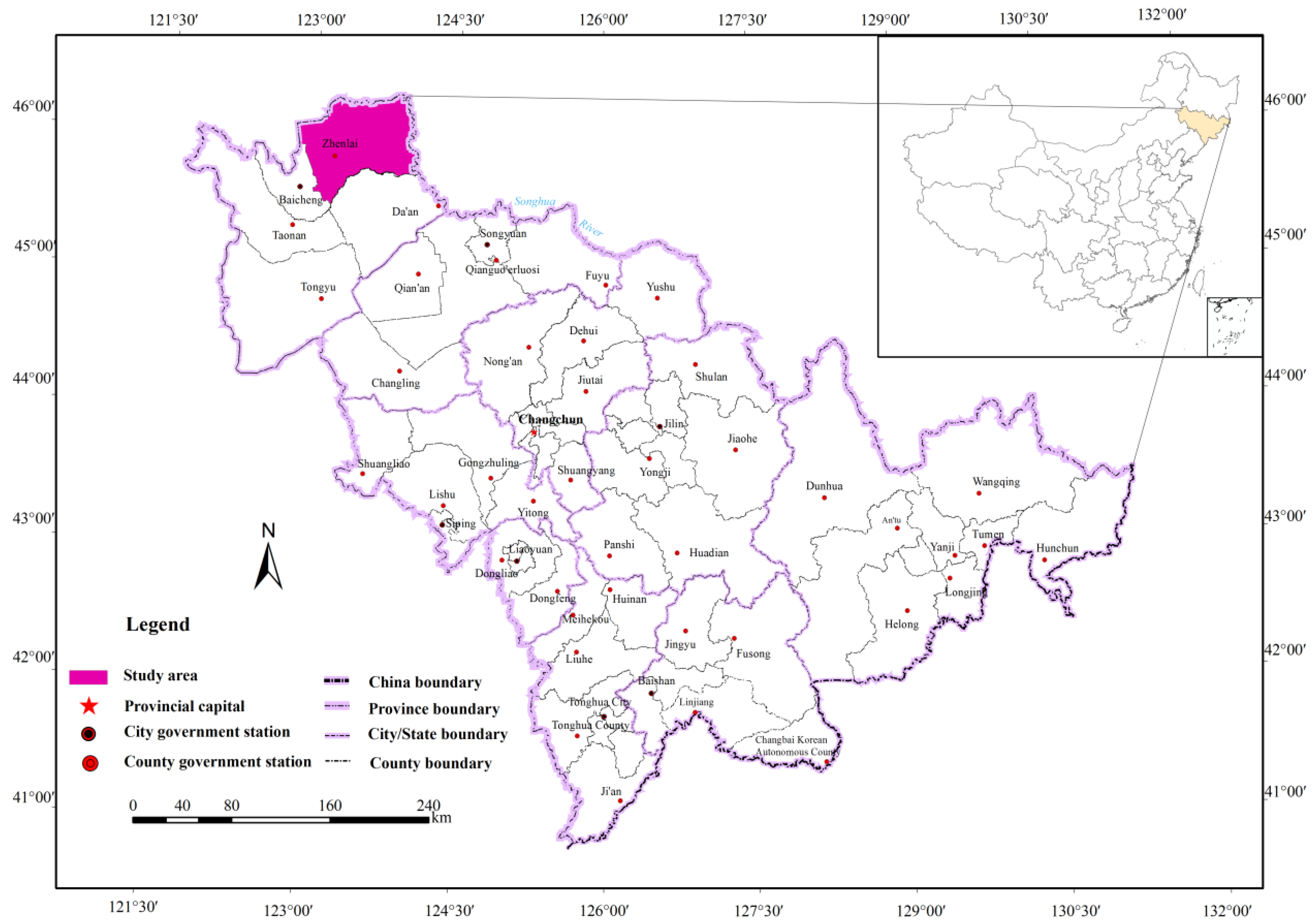
2.1. Study Area

2.2. Data
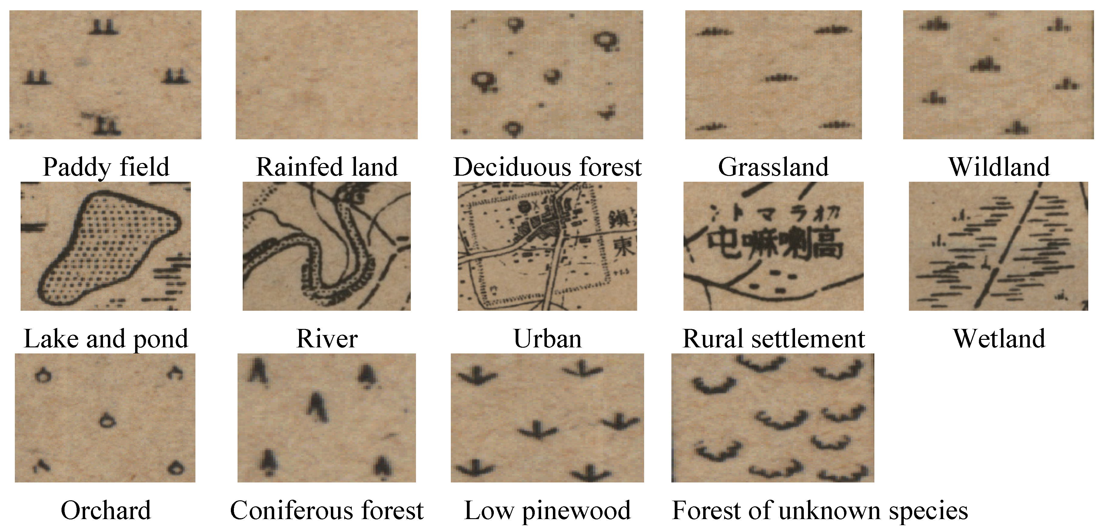
2.3. Classification System


| Code | Name of the land categories | Types in remote sensing images | Types in topographic maps |
|---|---|---|---|
| 1 | arable land | paddy field | paddy field |
| rainfed land | rainfed land | ||
| 2 | forest land | closed forest land | deciduous forest, coniferous forest, low pinewood |
| shrubbery | – | ||
| sparse wood land | – | ||
| other forest land | orchards, forest of unknown species | ||
| 3 | grassland | high coverage grassland | grassland |
| moderate coverage grassland | wildland | ||
| low coverage grassland | |||
| 4 | water | river | river |
| lake | lake, swag | ||
| swag | – | ||
| beachland | – | ||
| 5 | settlement | urban | urban |
| rural settlement | rural settlement | ||
| other construction | – | ||
| 6 | wetland | wetland | wetland |
| 7 | other unused land | sand | – |
| saline-alkali land | |||
| bare land |
2.4. Methods
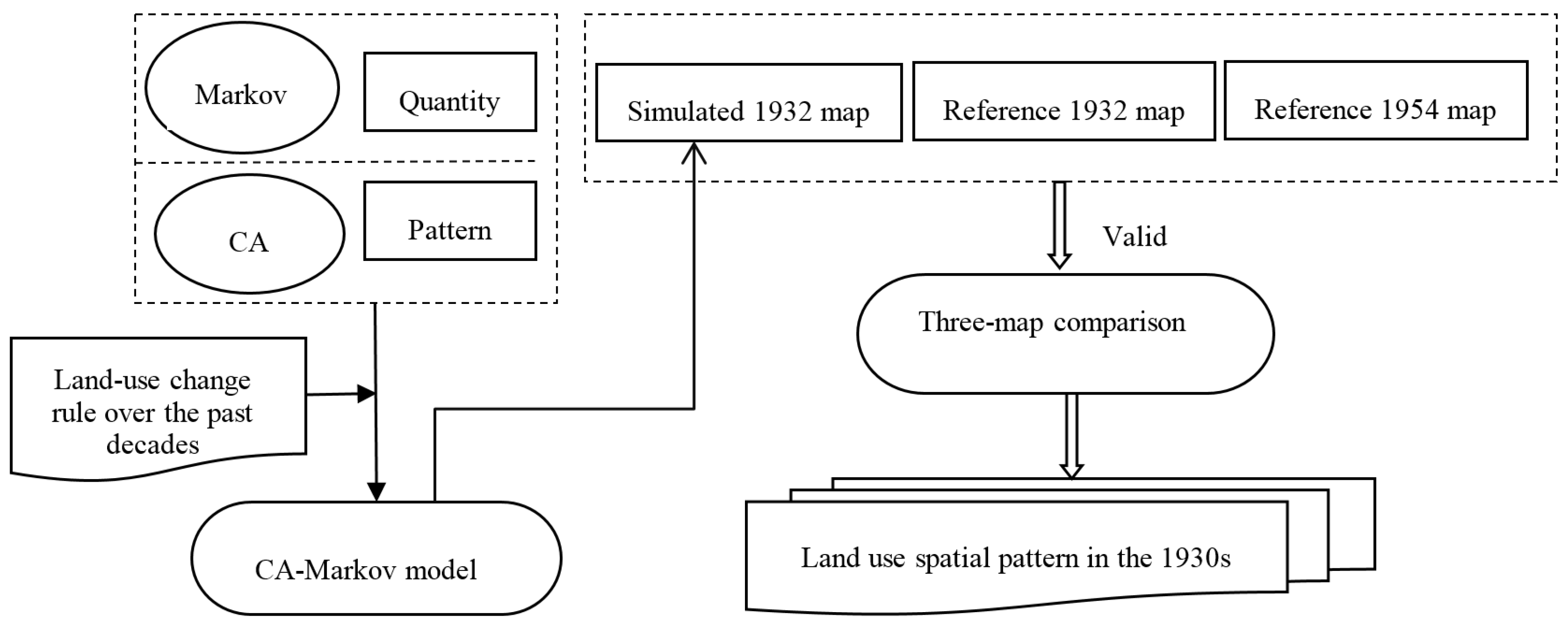
2.4.1. CA-Markov Model
2.4.2. Three-Map Comparison

3. Results


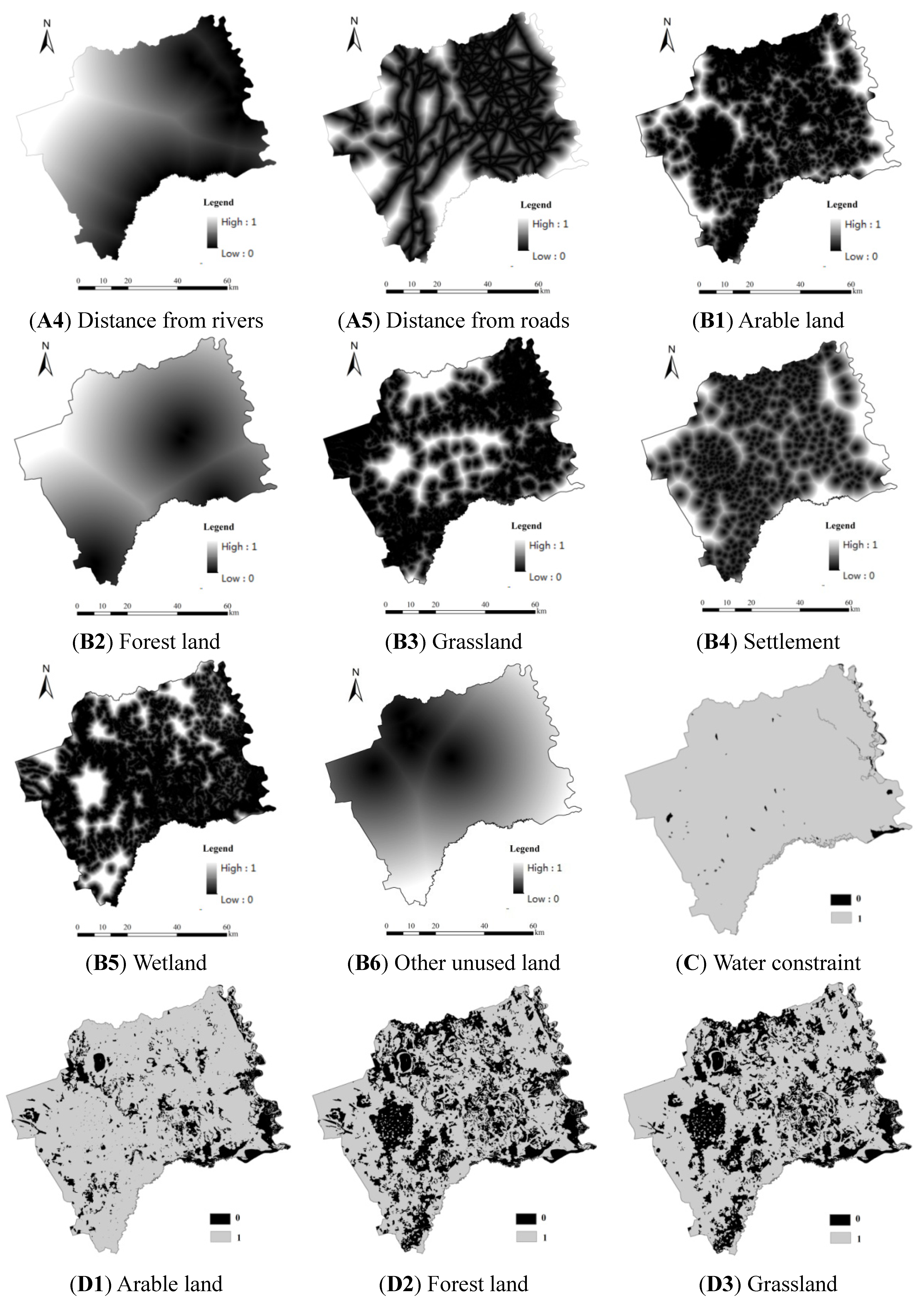
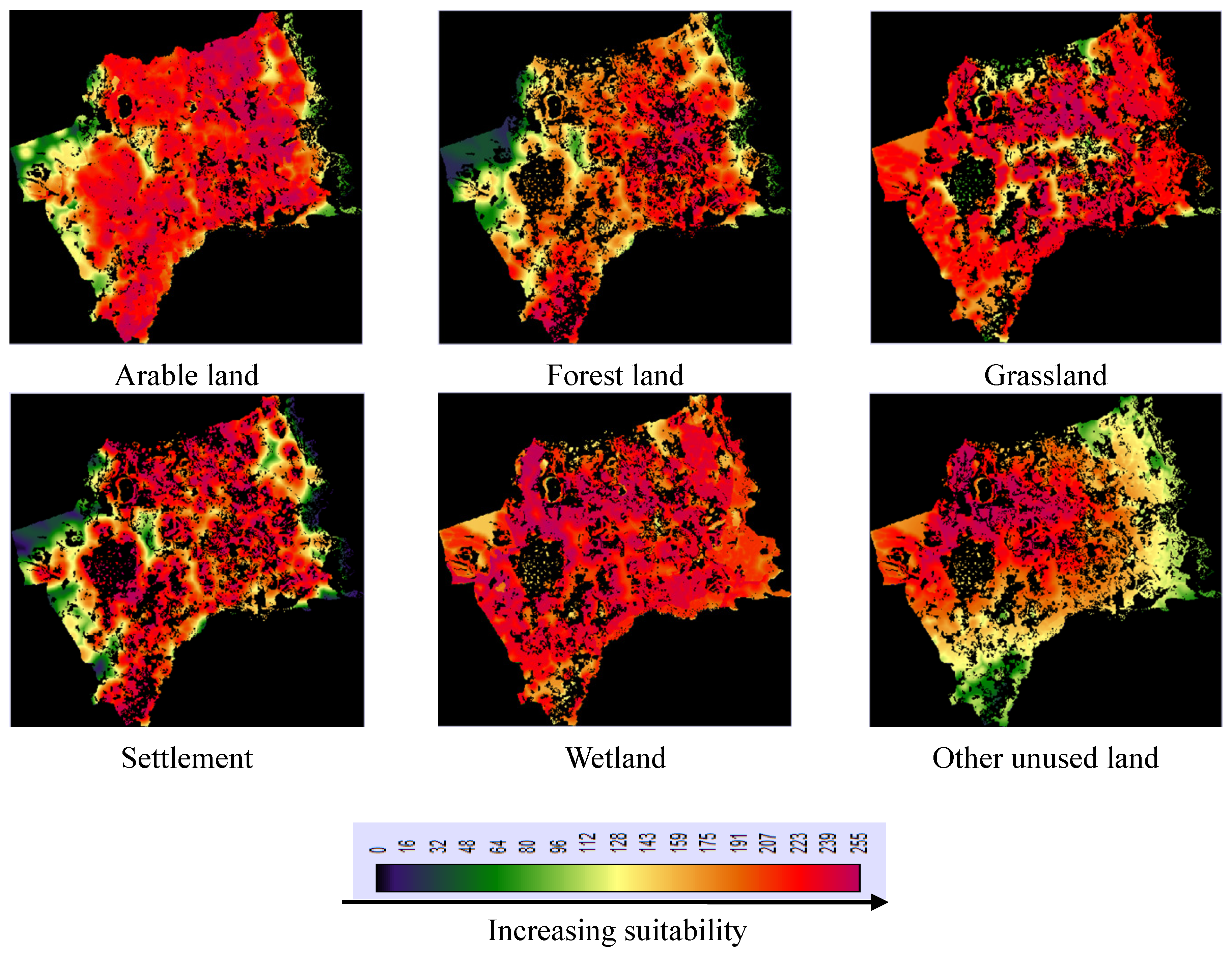
| Factors | Arable land | Forest | Grassland | Settlement | Wetland | Other unused land | |
|---|---|---|---|---|---|---|---|
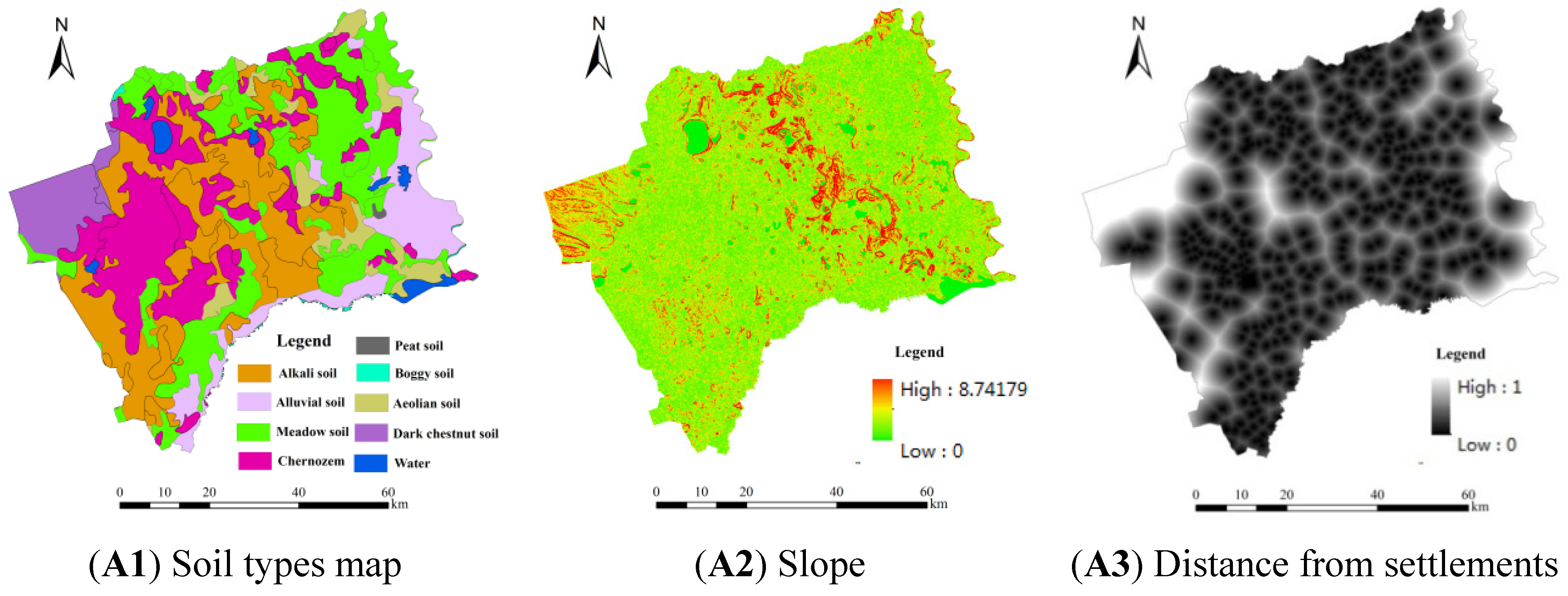
| Driving factors | Soil | 0.249 | 0.139 | 0.051 | 0.042 | 0.268 | 0.103 |
| Slope | 0.036 | 0.025 | 0.071 | – | 0.246 | – | |
| Distance from river | 0.096 | – | 0.099 | – | – | – | |
| Distance from roads | 0.092 | 0.072 | – | 0.124 | – | – | |
| Distance from settlement | 0.226 | 0.427 | – | 0.514 | – | – | |
| Spatial autocorrelation factors | Arable land | 0.301 | – | – | – | – | – |
| Forest land | – | 0.337 | – | – | – | – | |
| Grassland | – | – | 0.426 | – | 0.164 | 0.124 | |
| Settlement | – | – | – | 0.320 | – | – | |
| Wetland | – | – | 0.189 | – | 0.247 | 0.205 | |
| Other unused land | – | – | 0.164 | – | 0.075 | 0.568 | |


4. Discussion

| Final year (1932) | Initial total | Gross loss | |||||||
|---|---|---|---|---|---|---|---|---|---|
| Arable land | Forest | Grassland | Water | Settlement | Unused land | ||||
| Initial year (1954) | Arable land | 85202.00 | 122.19 | 76904.66 | 461.23 | 1026.98 | 3638.65 | 167355.71 | 82153.71 |
| 129195.45 | 0.56 | 34966.03 | 522.39 | 509.08 | 1735.09 | 166928.60 | 37733.15 | ||
| Forest | 143.27 | 76.74 | 252.40 | 0.00 | 16.24 | 0.00 | 488.65 | 411.91 | |
| 50.24 | 369.53 | 35.54 | 0.00 | 2.51 | 27.82 | 485.63 | 116.11 | ||
| Grassland | 24937.32 | 534.41 | 123704.28 | 1234.24 | 334.95 | 11626.66 | 162371.86 | 38667.58 | |
| 2017.96 | 238.00 | 152382.29 | 1325.70 | 82.71 | 7307.26 | 163353.92 | 10971.63 | ||
| Water | 3788.96 | 0.00 | 16556.56 | 2797.54 | 64.72 | 2792.23 | 26000.01 | 23202.47 | |
| 2125.27 | 0.00 | 4155.68 | 11048.21 | 13.39 | 8459.47 | 25802.01 | 14753.80 | ||
| Settlement | 1422.64 | 0.00 | 1192.72 | 2.93 | 275.85 | 50.44 | 2944.58 | 2668.73 | |
| 1219.25 | 3.89 | 670.57 | 1.70 | 969.07 | 78.82 | 2943.29 | 1974.22 | ||
| Unused land | 28250.58 | 148.62 | 127728.90 | 2263.89 | 664.62 | 13388.77 | 172445.37 | 159056.60 | |
| 12478.79 | 3.04 | 19363.19 | 2612.29 | 95.72 | 137539.71 | 172092.73 | 34553.02 | ||
| Initial total | 143744.76 | 881.97 | 346339.52 | 6759.83 | 2383.36 | 31496.74 | 531606.17 | 306161.00 | |
| 147086.96 | 615.01 | 211573.28 | 15510.29 | 1672.48 | 155148.16 | 531606.17 | 100101.93 | ||
| Gross Gain | 58542.77 | 805.23 | 222635.24 | 3962.29 | 2107.51 | 18107.97 | 306161.00 | – | |
| 17891.51 | 245.48 | 59191.00 | 4462.08 | 703.41 | 17608.45 | 100101.93 | – | ||

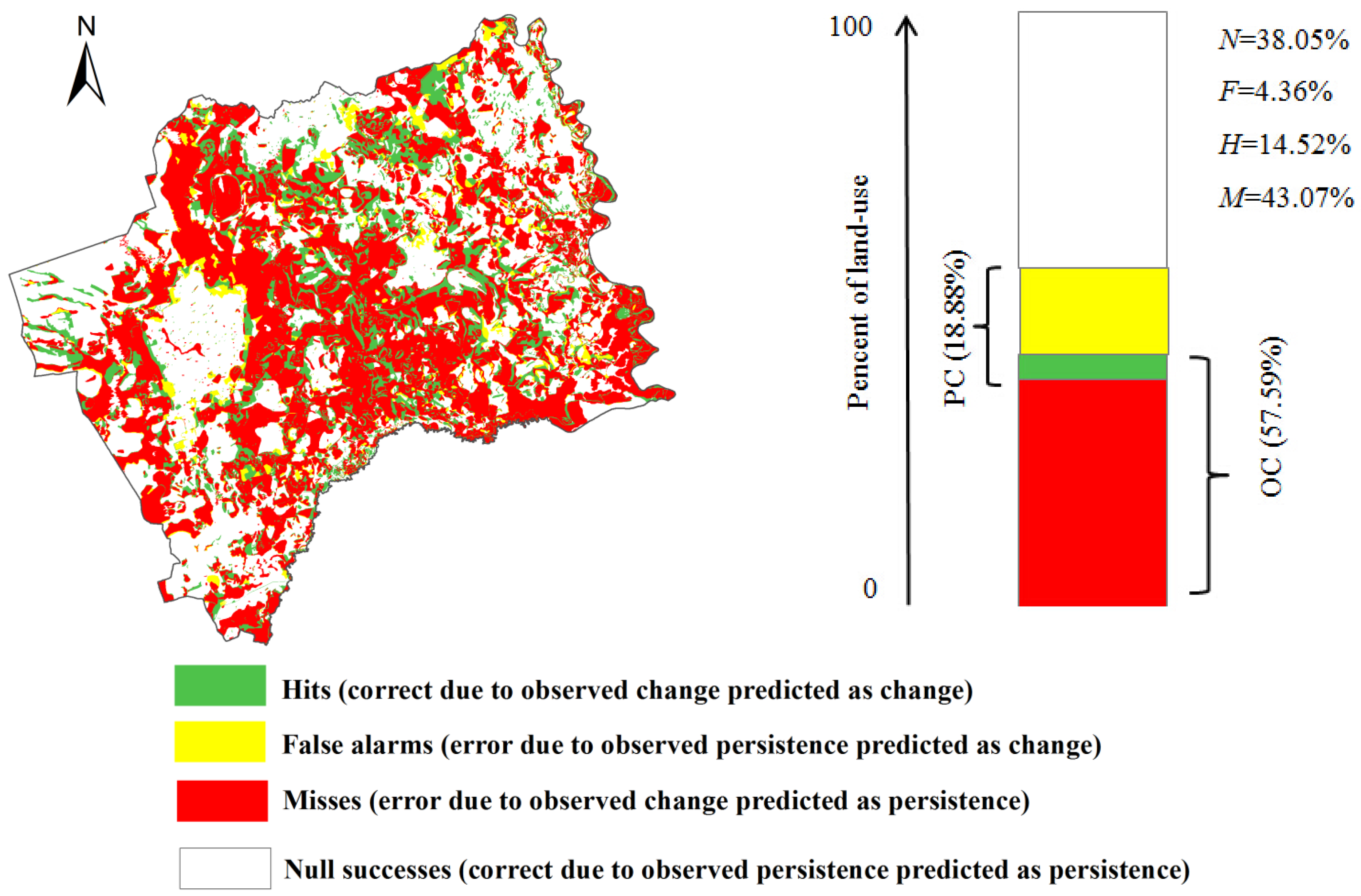
| Index | Value (%) | Index | Value (%) | Index | Value (%) | Index | Value |
|---|---|---|---|---|---|---|---|
| H | 14.52 | OC | 57.59 | EQ | 38.71 | HOC | 0.252 |
| M | 43.07 | PC | 18.88 | EA | 8.72 | MOC | 0.748 |
| F | 4.36 | T | 47.43 | – | – | FOC | 0.076 |
| N | 38.05 | FOM | 23.44 | – | – | – | – |
5. Conclusions
- (1)
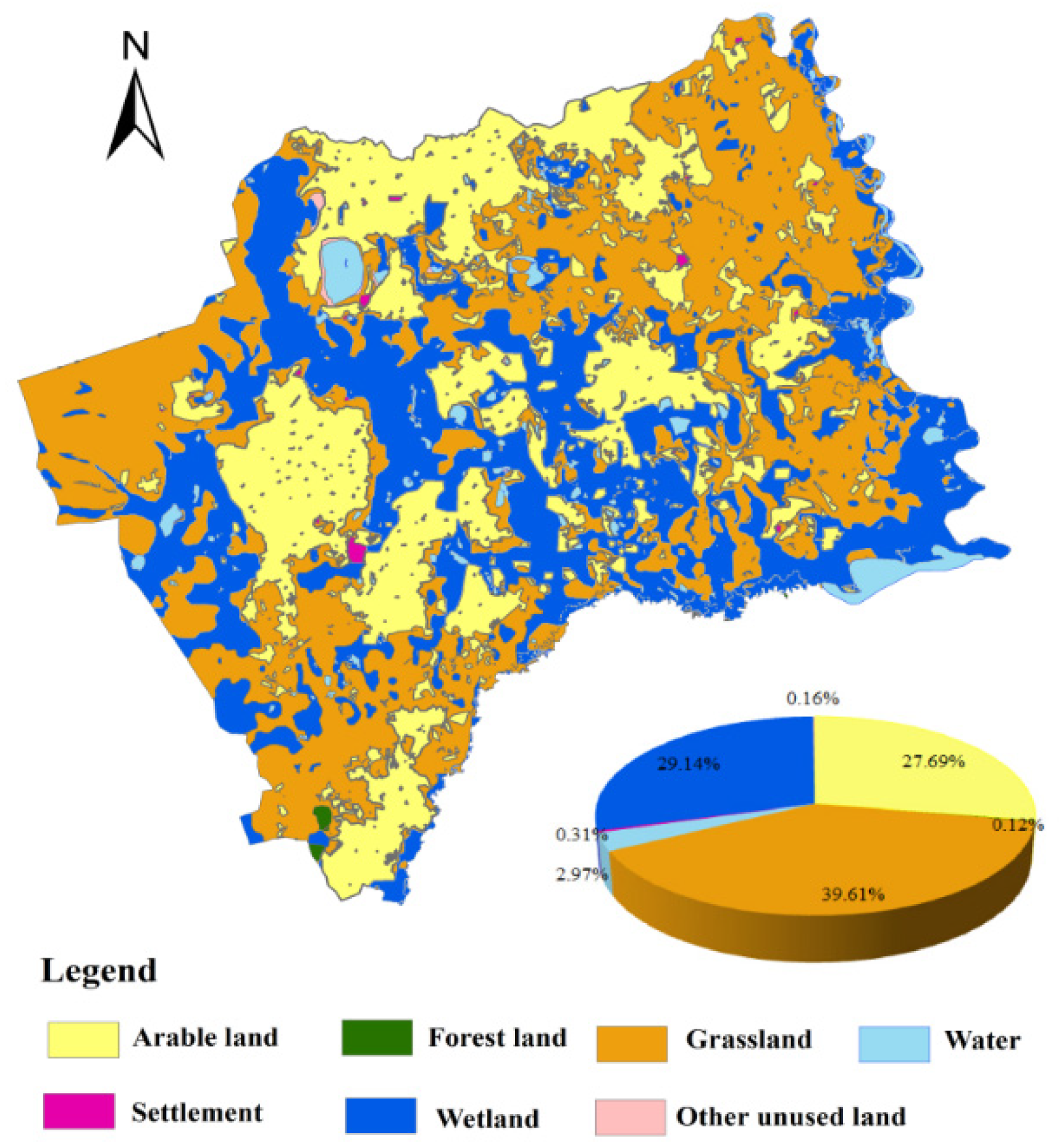
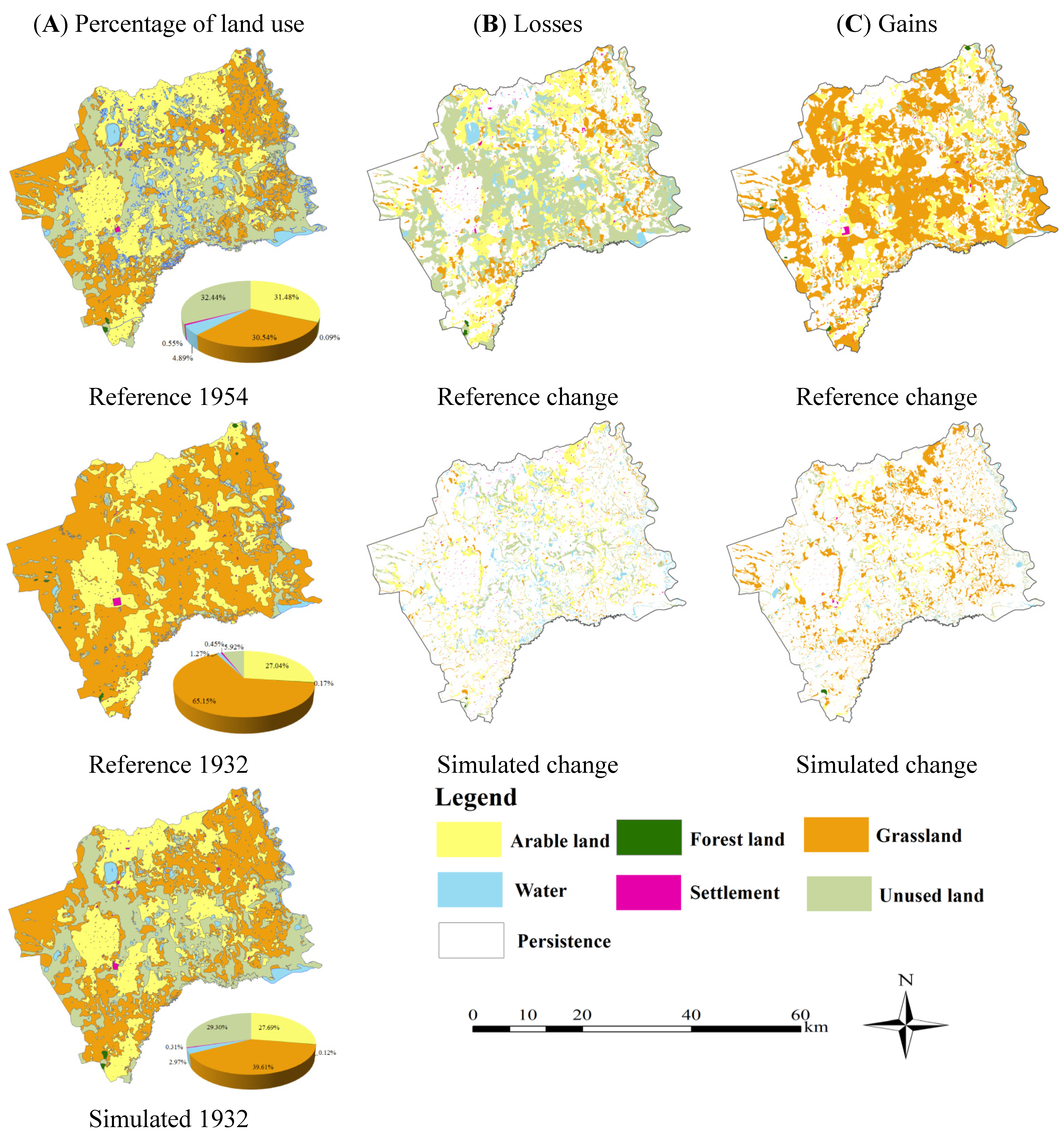
- The CA-Markov land cover change model can be simultaneously applicable to spatial reconstructions of various land cover types. The results of historical reconstruction showed that grassland occupied the largest percentage of the study area, followed by wetland and arable land. Other land categories, however, occupied relatively small areas.
- (2)
- The total change area for the reference change between 1954 and 1932 is 306,161.00 ha while it is only 100,101.93 ha for the simulated change. Gross losses and gross gains were mainly distributed in the middle of the study area and the areas near rivers and lakes. Arable land expanded at the expense of grassland due to the fast population growth during this period. The proportional area of water bodies increased slightly due to the increase of the precipitation. A large amount of grassland was converted into other unused land from 1932 to 1954 in both change maps, especially in the reference change, showing environmental degradation in the study area.
- (3)
- The figure of merit of the model was 23.44%. The relative error due to allocation was 8.72% while the error due to quantity was 38.71% because of the inconsistencies among time points concerning the definitions of categories in the maps. The major differences among the three maps have less to do with the simulation model and more to do with the inconsistencies among the land categories during the study period, especially for the grassland and unused land. The grassland in the topographic maps is often mixed with other land covers and its boundaries are not easy to determine. Besides, most of grassland in these maps is often judged as wildland, resulting in difficulty to extract and digitize the spatial explicit grassland data. It is important to choose a reference map with high accuracy in model validation using the three-map comparison methodology, however, it is very difficult for researchers to collect and obtain a suitable reference map in validation of reconstruction model due to the limitation of available historical data.
- (4)
- Historical topographic maps have a variety of limitations that must be considered to accurately interpret apparent land cover change. Each map shows its own land cover classes mainly based on its purpose and criteria. Different information provided by topographic maps and remote sensing images must be recognized, because of their intended uses. Blending different data can extend information about environmental change across a broad range of temporal and spatial scales. And then by combining multi-source data and information, a more complete picture of land use and land cover change can be obtained.
Acknowledgments
Author Contributions
Conflicts of Interest
References
- Lambin, E.F. Modelling and monitoring land-cover change processes in tropical regions. Prog. Phys. Geogr. 1997, 21, 375–393. [Google Scholar] [CrossRef]
- Turner, B.L.; Lambin, E.F.; Reenberg, A. The emergence of land change science for global environmental change and sustainability. Proc. Nat. Acad. Sci. USA 2007, 104, 20666–20671. [Google Scholar] [CrossRef] [PubMed]
- Foster, D.R.; Swanson, F.; Aber, J.; Burke, I.; Brokaw, N.; Tilman, D.; Knapp, A. The importance of land-use legacies to ecology and conservation. Bioscience 2003, 53, 77–88. [Google Scholar] [CrossRef]
- Gragson, T.L.; Bolstad, P.V. Land use legacies and the future of southern Appalachia. Soc. Nat. Resour. 2006, 19, 175–190. [Google Scholar] [CrossRef]
- Lambin, E.F.; Turner, B.L.; Geist, H.J.; Agbola, S.B.; Angelsen, A.; Bruce, J.W.; Coomes, O.T.; Dirzo, R.; Fischer, G.; Folke, C.; et al. The causes of land-use and land-cover change: Moving beyond the myths. Glob. Environ. Change 2001, 11, 261–269. [Google Scholar] [CrossRef]
- Deng, X.Z.; Zhao, C.H.; Lin, Y.Z.; Zhang, T.; Qu, Y.; Zhang, F.; Wang, Z.; Wu, F. Downscaling the impacts of large-scale LUCC on surface temperature along with IPCC RCPs: A global perspective. Energies 2014, 7, 2720–2739. [Google Scholar] [CrossRef]
- Arora, V.K.; Montenegro, A. Small temperature benefits provided by realistic afforestation efforts. Nat. Geosci. 2011, 4, 514–518. [Google Scholar] [CrossRef]
- Oldfield, F.; Dearing, J.A.; Gaillard, M.J.; Bugmann, H. Ecosystem processes and human dimensions—The scope and future of HITE (Human Impacts on Terrestrial Ecosystems. PAGES Newsl. 2000, 8, 21–23. [Google Scholar]
- Ramankutty, N.; Foley, J.A. Estimating historical changes in global land cover: Croplands from 1700 to 1992. Glob. Biogeochem. Cycles 1999, 13, 997–1027. [Google Scholar] [CrossRef]
- Petit, C.C.; Lambin, E.F. Long-term land-cover changes in the Belgian Ardennes (1775–1929): model-based reconstruction vs. historical maps. Glob. Change Biol. 2002, 8, 616–630. [Google Scholar] [CrossRef]
- Goldewijk, K.K.; Ramankutty, N. Land cover change over the last three centuries due to human activities: The availability of new global data sets. GeoJournal 2004, 61, 335–344. [Google Scholar] [CrossRef]
- Pongratz, J.; Reick, C.; Raddatz, T.; Claussen, M. A reconstruction of global agricultural areas and land cover for the last millennium. Glob. Biogeochem. Cycles 2008, 22, 1–16. [Google Scholar]
- Hurtt, G.C.; Frolking, S.; Fearon, M.G.; Moore, B.; Shevliakova, E.; Malyshev, S.; Pacala, S.W.; Houghton, R.A. The underpinnings of land-use history: Three centuries of global gridded land-use transitions, wood-harvest activity, and resulting secondary lands. Glob. Change Biol. 2006, 12, 1208–1229. [Google Scholar] [CrossRef]
- Liu, M.; Tian, H. China’s land cover and land use change from 1700 to 2005: Estimations from high-resolution satellite data and historical archives. Glob. Biogeochem. Cycles 2010, 24, 1–18. [Google Scholar] [CrossRef]
- Ye, Y.; Fang, X.Q. Land use change in Northeast China in the twentieth century: A note on sources, methods and patterns. J. Hist. Geogr. 2009, 35, 311–329. [Google Scholar] [CrossRef]
- Ye, Y.; Fang, X.Q. Spatial pattern of land cover changes across Northeast China over the past 300 years. J. Hist. Geogr. 2011, 3, 408–417. [Google Scholar] [CrossRef]
- Pontius, R.G., Jr.; Cornell, J.D.; Hall, C.A.S. Modeling the spatial pattern of land-use change with GEOMOD2: Application and validation for Costa Rica. Agric. Ecosyst. Environ. 2001, 85, 191–203. [Google Scholar] [CrossRef]
- Bolliger, J.; Schulte, L.A.; Burrows, S.N.; Sickley, T.A.; Mladenoff, D.J. Assessing ecological restoration potentials of Wisconsin (USA) using historical landscape reconstructions. Restor. Ecol. 2004, 12, 124–142. [Google Scholar] [CrossRef]
- Wulf, M.; Sommer, M.; Schmidt, R. Forest cover changes in the Prignitz region (NE Germany) between 1790 and 1960 in relation to soils and other driving forces. Landsc. Ecol. 2010, 25, 299–313. [Google Scholar] [CrossRef]
- Skaloš, J.; Weber, M.; Lipský, Z.; Trpáková, I.; Šantrůčková, M.; Uhlířová, L.; Kukla, P. Using old military survey maps and orthophotograph maps to analyse long-term land cover changes—Case study (Czech Republic). Appl. Geogr. 2011, 31, 426–438. [Google Scholar] [CrossRef]
- Bender, O.; Boehmerb, H.J.; Jens, D.; Schumacher, K.P. Using GIS to analyse long-term cultural landscape change in Southern Germany. Landsc. Urban Plan. 2005, 70, 111–125. [Google Scholar] [CrossRef]
- Boucher, Y.; Arseneault, D.; Sirois, L.; Blais, L. Logging pattern and landscape changes over the last century at the boreal and deciduous forest transition in Eastern Canada. Landsc. Ecol. 2009, 24, 171–184. [Google Scholar] [CrossRef]
- Hamre, L.N.; Domaas, S.T.; Austad, I.; Rydgren, K. Land-cover and structural changes in a western Norwegian cultural landscape since 1865, based on an old cadastral map and a field survey. Landsc. Ecol. 2007, 22, 1563–1574. [Google Scholar] [CrossRef]
- He, F.N.; Li, S.C.; Zhang, X.Z. The reconstruction of cropland area and its spatial distribution pattern in the mid-northern Song dynasty. Acta Geogr. Sin. 2011, 66, 1531–1539. (In Chinese) [Google Scholar]
- Kumar, S.; Merwade, V.; Rao, P.S.C.; Pijanowski, B.C. Characterizing long-term land use/cover change in the United States from 1850 to 2000 using a nonlinear bi-analytical model. AMBIO 2013, 42, 285–297. [Google Scholar] [CrossRef] [PubMed]
- Yang, Y.Y.; Zhang, S.W.; Yang, J.C.; Chang, L.P.; Bu, K.; Xing, X.S. A review of historical reconstruction methods of land use/land cover. J. Geogr. Sci. 2014, 24, 746–766. [Google Scholar] [CrossRef]
- Fuchs, R.; Herold, M.; Verburg, P.H.; Clevers, J.G.P.W. A high-resolution and harmonized model approach for reconstructing and analyzing historic land changes in Europe. Biogeosc. Discuss. 2012, 9, 14823–14866. [Google Scholar] [CrossRef] [Green Version]
- Wang, S.Q.; Zheng, X.Q.; Zang, X.B. Accuracy assessments of land use change simulation based on Markov-cellular automata model. Procedia Environ. Sci. 2012, 13, 1238–1245. [Google Scholar] [CrossRef]
- Pontius, G.R., Jr.; Malanson, J. Comparison of the structure and accuracy of two land change models. Int. J. Geogr. Inf. Sci. 2005, 19, 243–265. [Google Scholar] [CrossRef]
- Pontius, R.G., Jr.; Millones, M. Death to Kappa: Birth of quantity disagreement and allocation disagreement for accuracy assessment. Int. J. Remote Sens. 2011, 32, 4407–4429. [Google Scholar] [CrossRef]
- Chen, H.; Pontius, R.G., Jr. Diagnostic tools to evaluate a spatial land change projection along a gradient of an explanatory variable. Landsc. Ecol. 2010, 25, 1319–1331. [Google Scholar] [CrossRef]
- Pontius, R.G., Jr.; Boersma, W.; Castella, J.C.; Clarke, K.; de Nijs, T.; Dietzel, C.; Duan, Z.Q.; Fotsing, E.; Goldstein, N.; Kok, K.; et al. Comparing the input, output, and validation maps for several models of land change. Ann. Reg. Sci. 2008, 42, 11–37. [Google Scholar] [CrossRef]
- García, A.M.; Santé, I.; Boullón, M.; Crecente, R. A comparative analysis of cellular automata models for simulation of small urban areas in Galicia, NW Spain. Comput. Environ. Urban Syst. 2012, 36, 291–301. [Google Scholar] [CrossRef]
- Chen, H.; Pontius, R.G., Jr. Sensitivity of a land change model to pixel resolution and precision of the independent variable. Environ. Model. Assess. 2011, 16, 37–52. [Google Scholar] [CrossRef]
- Zhang, Y.J.; Gao, Z.J.; Yu, H. Local Record of Zhenlai County; Jilin People’s Press: Changchun, China, 1995. (In Chinese) [Google Scholar]
- Bai, S.Y.; Zhang, S.W. The discussion of the method of land utilization spatial information reappearance of history period. J. Arid Land Resour. Environ. 2004, 18, 77–80. (In Chinese) [Google Scholar]
- Bai, S.Y.; Zhang, S.W.; Zhang, Y.Z. Study on the method of diagnose the plowland spacial distribution in historical era. Syst. Sci. Compr. Stud. Agric. 2005, 21, 252–255. (In Chinese) [Google Scholar]
- Liu, J.Y.; Liu, M.L.; Zhuang, D.F.; Zhang, Z.X.; Deng, X.Z. Study on spatial pattern of land-use change in China during 1995–2000. Sci. China 2003, 46, 374–384. [Google Scholar] [CrossRef]
- Pontius, R.G., Jr.; Shusas, E.; McEachern, M. Detecting important categorical land changes while accounting for persistence. Agric. Ecosyst. Environ. 2004, 101, 251–268. [Google Scholar] [CrossRef]
- Santé, I.; García, A.M.; Miranda, D.; Crecente, R. Cellular automata models for the simulation of real-world urban processes: A review and analysis. Landsc. Urban Plan. 2010, 96, 108–122. [Google Scholar] [CrossRef]
- Pontius, R.; Peethambaram, S.; Castella, J.-C. Comparison of three maps at multiple resolutions: A case study of land change simulation in Cho Don District, Vietnam. Ann. Assoc. Am. Geogr. 2011, 101, 45–62. [Google Scholar] [CrossRef]
- Yang, Y.Y.; Zhang, S.W.; Wang, D.Y.; Yang, J.C.; Xing, X.X. Spatiotemporal changes of farming-pastoral ecotone in Northern China, 1954–2005: A case study in Zhenlai County, Jilin Province. Sustainability 2014, 7, 1–22. [Google Scholar] [CrossRef]
- Poska, A.; Sepp, E.; Veski, S.; Koppel, K. Using quantitative pollen-based land-cover estimations and a spatial CA_Markov model to reconstruct the development of cultural landscape at Rõuge, South Estonia. Veget. Hist. Archaeobot. 2008, 17, 527–541. [Google Scholar] [CrossRef]
- Samat, N.; Hasni, R.; Elhadary, Y.A.E. Modelling land use changes at the peri-urban areas using geographic information systems and cellular automata model. J. Sustain. Dev. 2011, 4, 72–84. [Google Scholar] [CrossRef]
- Lin, N.F.; Tang, J.; Wang, X.G.; Bian, J.M.; Li, Z.Y.; Wang, C.Y. Constructions of a geo-information atlas-spatial analysis model toward a perspective of the spatial pattern changes in land use. Quat. Sci. 2009, 29, 711–723. (In Chinese) [Google Scholar]
- Gimmi, U.; Bürgi, M.; Stuber, M. Reconstructing anthropogenic disturbance regimes in forest ecosystems: A case study from the Swiss Rhone valley. Ecosystems 2008, 11, 113–124. [Google Scholar] [CrossRef]
- Wang, Z.M.; Zhang, B.; Song, K.S.; Liu, D.W. Extracting land use information based on topographical map and knowledge rules. Geo-inf. Sci. 2008, 10, 67–73. (In Chinese) [Google Scholar]
- Gao, P.; Mu, X.M.; Wang, F.; Wang, S.Y. Trend analysis of precipitation in Northeast China in recent 100 years. J. China Hydrol. 2010, 30, 80–84. (In Chinese) [Google Scholar]
- Sun, F.H.; Yuan, J.; Lu, S. The change and test of climate in Northeast China over the last 100 years. Clim. Environ. Res. 2006, 11, 101–108. (In Chinese) [Google Scholar]
© 2015 by the authors; licensee MDPI, Basel, Switzerland. This article is an open access article distributed under the terms and conditions of the Creative Commons Attribution license (http://creativecommons.org/licenses/by/4.0/).
Share and Cite
Yang, Y.; Zhang, S.; Yang, J.; Xing, X.; Wang, D. Using a Cellular Automata-Markov Model to Reconstruct Spatial Land-Use Patterns in Zhenlai County, Northeast China. Energies 2015, 8, 3882-3902. https://doi.org/10.3390/en8053882
Yang Y, Zhang S, Yang J, Xing X, Wang D. Using a Cellular Automata-Markov Model to Reconstruct Spatial Land-Use Patterns in Zhenlai County, Northeast China. Energies. 2015; 8(5):3882-3902. https://doi.org/10.3390/en8053882
Chicago/Turabian StyleYang, Yuanyuan, Shuwen Zhang, Jiuchun Yang, Xiaoshi Xing, and Dongyan Wang. 2015. "Using a Cellular Automata-Markov Model to Reconstruct Spatial Land-Use Patterns in Zhenlai County, Northeast China" Energies 8, no. 5: 3882-3902. https://doi.org/10.3390/en8053882