1. Introduction
As a result of recent strong interest in solar energy, experimental solar radiation data for potential areas of solar power generation were collected and used in a solar energy system design. However, in many cases, those radiation data are insufficient. The operating characteristics and the performance of solar energy systems are unstable, since the amount of solar radiation gain and its pattern vary due to the changing of the solar collector efficiency or the thermal storage heat loss of a solar thermal energy system [
1,
2]. The data of solar radiation change in a short time are not cumulated for most potential solar energy system installation areas.
In general, solar systems use direct solar radiation observation, indirect solar radiation data, which are derived from observed temperature, humidity and other weather factors, or the averaged solar radiation data [
3]. With observed solar radiation data, realistic system simulation and annual gain analysis are possible. Indirect solar energy estimate studies are conducted due to the lack of the actual solar radiation data [
4,
5,
6,
7,
8]. Those estimations use observed weather variables, such as sunshine [
9,
10], temperature [
11,
12] or cloud [
11,
13,
14,
15]. Using direct and indirect weather data involves significant effort in choosing data from the large original dataset. Therefore, this approach is problematic, since there are no criteria for sampling. The solar energy system is normally turned off when solar irradiation goes below a certain level (for example, 400 W/m
2), which means that the system is mainly operating during clear days. Freeman
et al. [
16] considered various ways of aggregating time-varying solar data and evaluated the energy output from a solar-thermal collector. They found that the extent of the error for the annual work output was caused by using averaged weather data.
The aim of this study is to add weather variability to a simple averaged solar radiation model; it will serve as a basis for the future development of an accurate solar radiation model for use in the design and development of new solar energy systems. To evaluate the proposed model, dynamic simulations of a solar organic Rankine cycle (SORC) system were conducted using an actual distribution of daily solar radiation, the proposed model and the simple sky model.
2. Numerical Modelling of Solar Radiation
The solar radiation model for a cloudy sky proposed in this study is based on the simple sky model [
3] that is generally used in solar energy simulations. The simple sky model is characterized by the parameters of the peak solar irradiance (
), the sunrise time (
and the sunset time (
) as follows:
where
is time. The peak solar irradiance is derived as equal total daily solar exposures between the observed value and the value from the simple sky model. The cloudiness (
M) is represented as the ratio of the peak solar irradiance (
) to the daily maximum extraterrestrial irradiance (
) as follows:
The extraterrestrial irradiance (
) is defined as the product of the solar constant (
I0, fixed as 1362), and the eccentricity correction factor (
E0) that is usually represented using a simple correlation (see Equation (3)). Thus, the extraterrestrial irradiance is given by:
where
is the number of the day in the year and
is the zenith angle, which is calculated from the function of local time and location [
3,
17].
As shown in Equation (1), the simple sky model consists of a single sinusoidal wave and therefore does not include the effects of weather variability.
To represent accurately the variation in the solar radiation due to weather changes, a superposition of multiple sinusoidal waves with different magnitudes and frequencies are considered. In this study, two sinusoidal waves are added to the simple sky model as follows:
where
a1 and
a2 are the amount of solar irradiance variation;
b1 and
b2 are the frequency of the weather changes and
c1 and
c2 are the rate of change in weather.
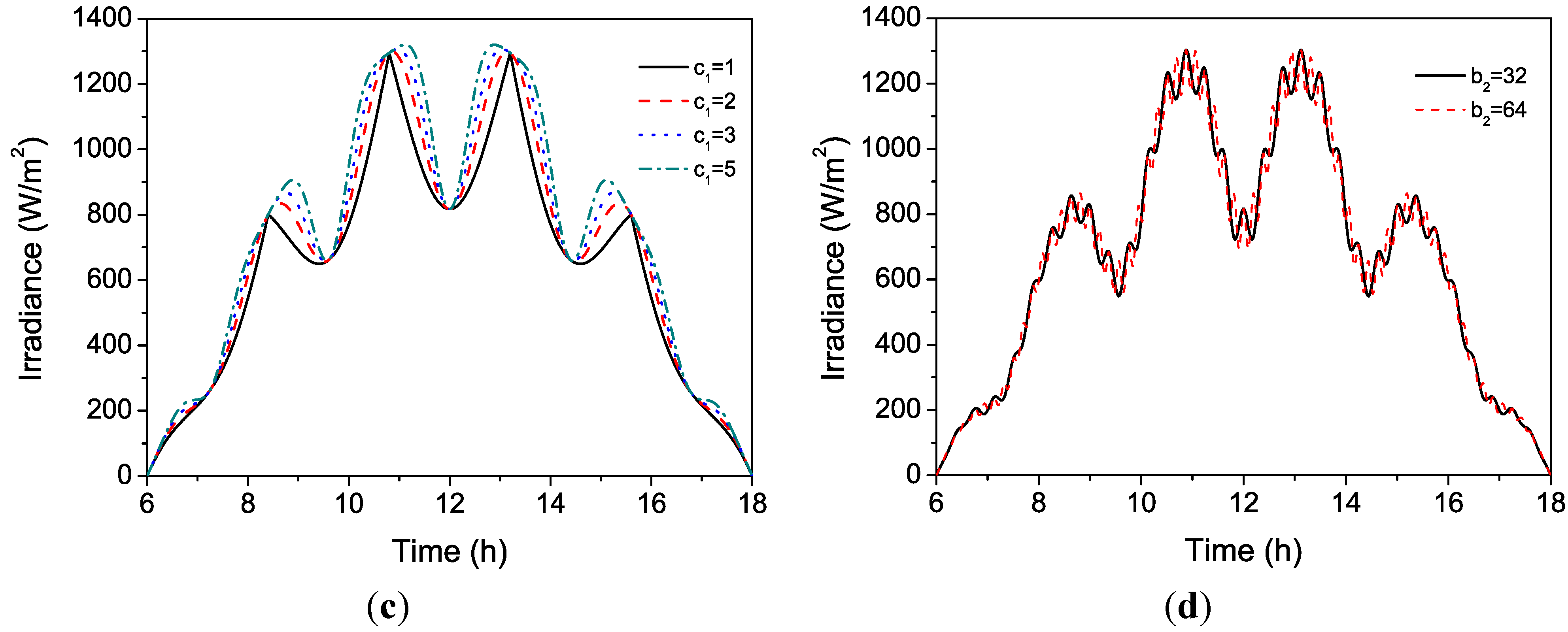
Thus, the proposed model includes long (subscript 1) and short (subscript 2) periods of weather variations. In order to see how model variables effect solar irradiance distribution, a case study was conducted, and
Figure 1 shows the distribution of solar radiation
Icloudy,sky for the various values of the parameters
a1,
b1,
c1 and
b2. The effect of variable a
1 is shown in
Figure 1a. A higher value of a
1 increases the depth of fluctuations.
Figure 1b shows the effect of the frequency of the long-term weather changes
b1. The number of
b1 indicates the number of fluctuations during a day.
Figure 1c illustrates the effect of long-term weather change rate
c1. An increase in
c1 results in a clear increase in total daily solar irradiance. The effect of the short period weather changes
b2 is shown in
Figure 1d. Similar to the case of
b1,
b2 represents the number of short-term fluctuations during a day.
Figure 1.
Solar radiation distributions obtained by the proposed model for the different values of the parameters in Equation (4): (a) M = 1, b1 = 5, c1 = 3, a2 = 0; (b) M = 1, a1 = 0.3, c1 = 3, a2 = 0; (c) M = 1, a1 = 0.3, b1 = 5, a2 = 0; (d) M = 1, a1 = 0.3, b1 = 5, c1 = 3, a2 = 0.1, c2 = 3.
Figure 1.
Solar radiation distributions obtained by the proposed model for the different values of the parameters in Equation (4): (a) M = 1, b1 = 5, c1 = 3, a2 = 0; (b) M = 1, a1 = 0.3, c1 = 3, a2 = 0; (c) M = 1, a1 = 0.3, b1 = 5, a2 = 0; (d) M = 1, a1 = 0.3, b1 = 5, c1 = 3, a2 = 0.1, c2 = 3.
Statistical indices are generally used for the characterization of solar radiation. The sky clearness index k is defined as the ratio of the actual received irradiance (instant global horizontal irradiance,
) to the maximum theoretically possible extraterrestrial irradiance (
):
The daily sky clearness index
is then derived from the integrals of the variables in Equation (5) [
3].
Kang and Tam [
18] proposed the daily probability of persistence (
POPD) index that describes the stability of the daily solar irradiance for a fixed one-minute time interval.
POPD calculates a possibility that adjacent instantaneous clearness indices are equal.
POPD is derived from the following procedure.
Calculate the instantaneous clearness index
for each time series.
Round off the value of k at the first decimal place (e.g., 0.1, 0.3, etc.).
Count the number of identical cases between adjacent time series.
Divide the counting number by the number of time series (POPD).
The higher value of
POPD indicates smaller weather variability. They also suggested a classification method based on
kD and
POPD to describe the daily weather variability and showed that the observed daily weather could be categorized into ten classes, as shown in
Table 1.
Table 1.
Classification parameters of solar radiation with
kD and
POPD [
18].
Table 1.
Classification parameters of solar radiation with kD and POPD [18].
| Class | kD | POPD | Description |
|---|
| 1 | kD > 0.6 | POPD > 0.9 | High quantity and high quality; sunny and steady sky conditions for almost the entire day |
| 2 | 0.3 < kD < 0.6 | POPD > 0.9 | Medium quantity and high quality; partly cloudy, but sky conditions are relatively steady for most of the day |
| 3 | kD < 0.3 | POPD > 0.9 | Low quantity and high quality; overcast, but sky conditions are relatively steady for most of the day |
| 4 | kD > 0.6 | 0.7 < POPD < 0.9 | High quantity and medium quality; sunny, but the sky conditions vary for part of the day |
| 5 | 0.3 < kD < 0.6 | 0.7 < POPD < 0.9 | Medium quantity and medium quality; partly cloudy and the sky conditions vary for part of the day |
| 6 | kD < 0.3 | 0.7 < POPD < 0.9 | Low quantity and medium quality; cloudy and the sky conditions vary |
| 7 | kD > 0.6 | 0.5 < POPD < 0.7 | High quantity and low quality; partly sunny with sky conditions varying significantly for most of the day |
| 8 | 0.3 < kD < 0.6 | 0.5 < POPD < 0.7 | Medium quantity and low quality; various degrees of cloudiness and the sky conditions varying significantly for most of the day |
| 9 | kD < 0.3 | 0.5 < POPD < 0.7 | Low quantity and low quality; various degrees of cloudiness, but high levels of fluctuations for the entire day |
| 10 | - | POPD < 0.5 | Very low quality |
In order to examine the feasibility of the proposed model, four cases of the observed hourly solar irradiance samples are simulated. The solar radiation data are given by the National Renewable Energy Laboratory (
http://www.nrel.gov/midc/) [
19,
20]. Each simulation curve is modelled according to the amount of solar irradiance (
kD) and the characteristics of long- and short-term fluctuations. First, model shape variables of
a1,
a2,
b1,
b2,
c1 and
c2 are selected to implement the fluctuation pattern, and then, the amount of solar irradiance is matched by varying the value of cloudiness
M. Solar radiation simulation variables and indices are shown in
Table 2, and the corresponding irradiance distributions are shown in
Figure 2.
Figure 2a shows the irradiance distribution of the observed data and the simple model for a sunny day. During the daytime, the simple model returns relatively higher value of irradiance than the observed data, which make the thermal system warm-up faster during simulation.
Figure 2b illustrates the irradiance distributions for a cloudy day. It is obvious that the proposed model does not match with fluctuations in various frequencies and intensities compared to the curves by the observed data exactly, but follows the tendency of the irradiance distribution. Meanwhile, similar to sunny day results, the simple model and the proposed model show larger irradiance during daytime.
Figure 2c,d shows that the irradiance distribution of cloudy days is overcast, which is common. In this case, the proposed model does not fit well (
Figure 2c). These kinds of weather changes can be simply implemented by removing fluctuation terms during, before or after a certain time (
Figure 2d).
Figure 2e,f illustrates the irradiance distribution of long-term large weather change conditions with short-term small fluctuations. Major differences between the cases are in the long term, such as the amount of solar irradiance (
a1) being 0.3 and 0.6 and the frequency of the weather changes being six and seven. In all cases, the simulated curves match with the observed one within a specific period of time.
Figure 2.
Solar radiation distributions for the actual weather data, the simple sky model and the proposed model as shown in
Table 2. Data (
a–
d) observed in Anatolia-Rancho Cordova, California (latitude: 38.546° N; longitude: 121.24° W; elevation: 51 m; PST) [
20]. Data (
e,
f) observed in Golden, Colorado (latitude: 39.742° N; longitude: 105.18° W; elevation: 1828.8 m; MST) [
19].
Table 2.
Solar radiation simulation variables and indices.
Table 2.
Solar radiation simulation variables and indices.
| Data | Model | Variables | Indices |
|---|
| M | a1 | b1 | c1 | a2 | b2 | c2 | kD | POPD | Class |
|---|
| Case 1 | Observed | | | | | | | | 0.67 | 0.98 | 1 |
| | Simple | 0.67 | | | | | | | 0.67 | 0.99 | 1 |
| Case 2 | Observed | | | | | | | | 0.48 | 0.67 | 8 |
| | Simple | 0.46 | | | | | | | 0.48 | 0.99 | 2 |
| | Model | 0.81 | 0.2 | 8 | 3 | 0.6 | 60 | 3 | 0.48 | 0.67 | 8 |
| Case 3 | Observed | | | | | | | | 0.61 | 0.69 | 7 |
| | Simple | 0.61 | | | | | | | 0.61 | 0.99 | 1 |
| | Model 3-1 | 0.81 | 0.1 | 7 | 1 | 0.5 | 40 | 2 | 0.61 | 0.67 | 7 |
| | Model 3-2 * | 0.76 | 0.1 | 7 | 1 | 0.5 | 40 | 2 | 0.61 | 0.79 | 4 |
| Case 4 | Observed | | | | | | | | 0.72 | 0.78 | 4 |
| | Simple | 0.73 | | | | | | | 0.72 | 0.99 | 1 |
| | Model 4-1 | 0.86 | 0.3 | 6 | 2 | 0.1 | 64 | 2 | 0.72 | 0.90 | 1 |
| | Model 4-2 | 1.01 | 0.6 | 6 | 2 | 0.1 | 64 | 2 | 0.72 | 0.84 | 4 |
| | Model 4-3 | 0.86 | 0.3 | 7 | 2 | 0.1 | 64 | 2 | 0.72 | 0.89 | 4 |
| | Model 4-4 | 1.01 | 0.6 | 7 | 2 | 0.1 | 64 | 2 | 0.72 | 0.81 | 4 |
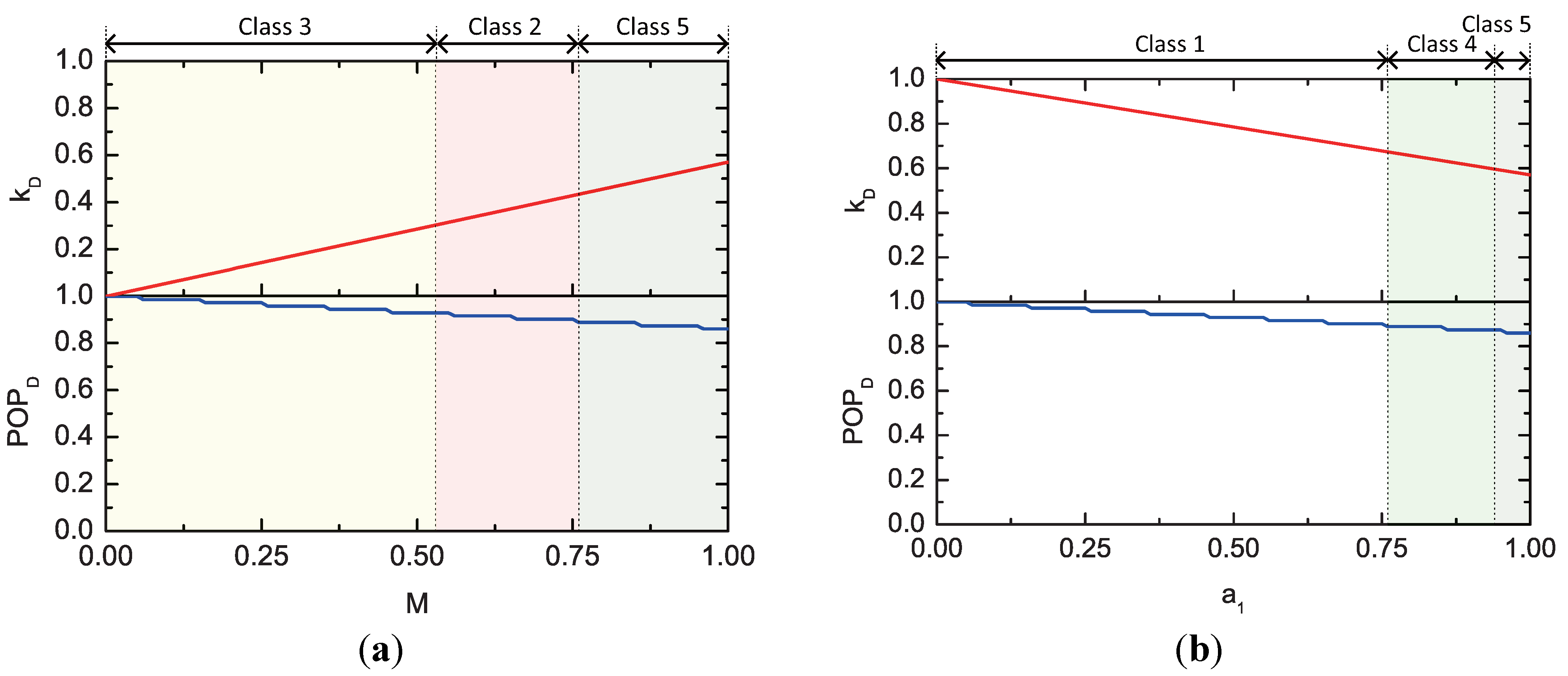
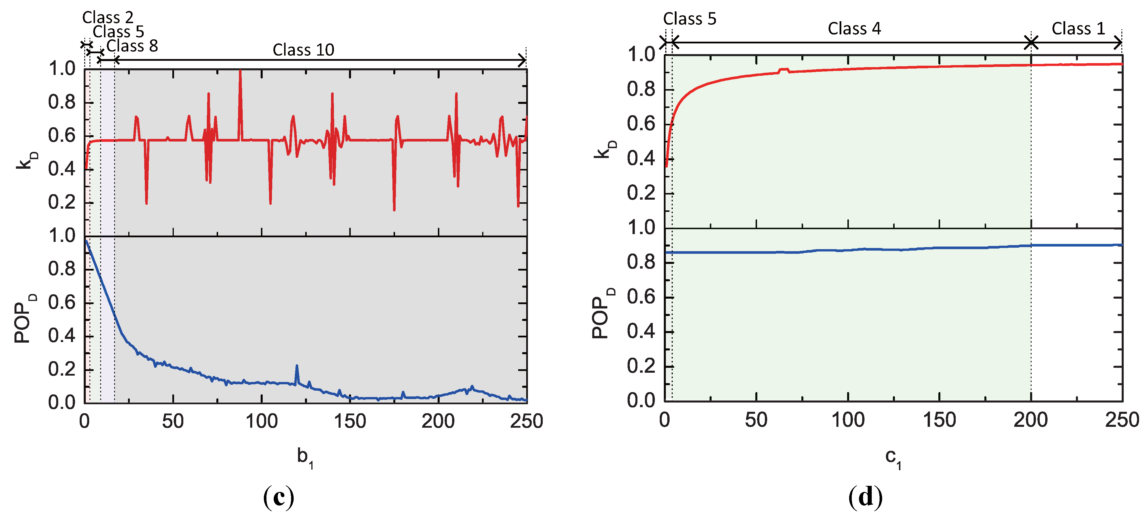
We investigate how different values of model parameters impact on the
kD and
POPD, and we evaluate the proposed model by comparing its results with weather conditions in the
kD-POPD classes.
Figure 3 shows the dependence of
kD,
POPD and
kD-POPD classes on the parameters of the variable weather model given by Equation (4). The values of
kD are strongly affected by the changes in the
M,
a1 and
c1 values, while the values of
POPD are mainly affected by the changes in the
b1 parameter. Thus, the results presented in
Figure 3 show that the proposed model can realize a wide range of weather changes for solar energy system simulations. Although the
kD-POPD Classes 6, 7 and 9 do not appear in the figure, the solar radiation distributions in those classes can be easily obtained by simultaneously changing two or more variables in Equation (4).
Figure 3.
Effects of the changes in (a) M, (b) a1, (c) b1 and (d) c1 on kD, POPD and the kD-POPD class for the base model with M = 1, a1 = 0.5, a2 = 0, b1 = 5, b2 = 0, c1 = 3 and c2 = 3.
Figure 3.
Effects of the changes in (a) M, (b) a1, (c) b1 and (d) c1 on kD, POPD and the kD-POPD class for the base model with M = 1, a1 = 0.5, a2 = 0, b1 = 5, b2 = 0, c1 = 3 and c2 = 3.
The weather simulation results show that the proposed model implements actual weather conditions to limited extent. In spite of these limitations, the proposed model could be applied to thermal system simulation, since the proposed model provides a tool for case studies beyond the intrinsic randomness of weather.
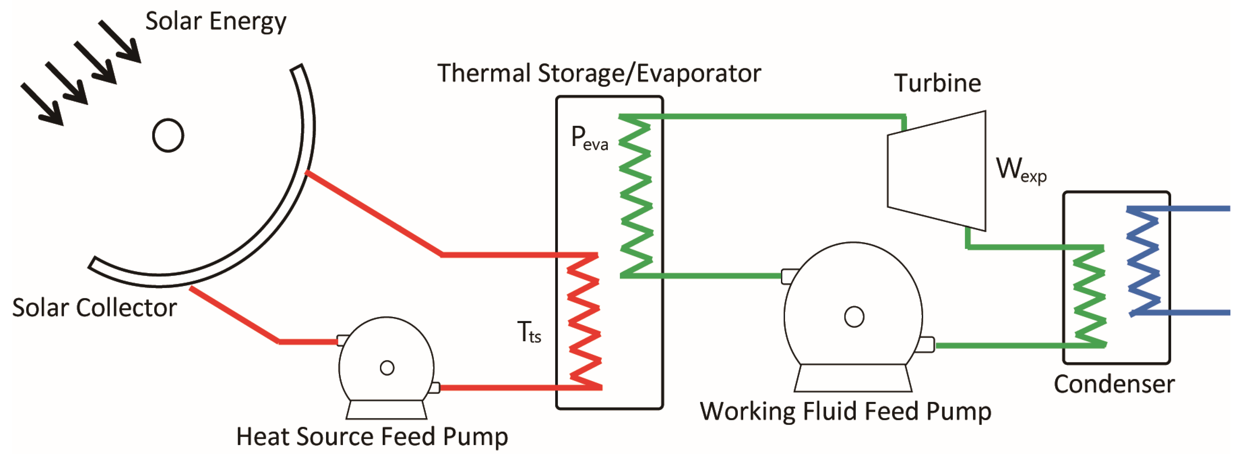
3. Application: Dynamic Simulation of SORC
In this chapter, a dynamic simulation of a solar organic Rankine cycle (SORC) system is conducted to figure out the differences between the simple model and the proposed model. The schematics of the SORC system is shown in
Figure 4. The ORC system is a type of Rankine cycle system that uses organic refrigerant as the working fluid. The change of the solar irradiance influences the operating characteristics of the SORC system, such as solar collector efficiency, thermal efficiency and system on/off frequency.
Figure 4.
Schematic diagram of the solar organic Rankine cycle (SORC) model.
Figure 4.
Schematic diagram of the solar organic Rankine cycle (SORC) model.
A lumped SORC model designed by Twomey
et al. for studying the relationship between the solar radiation pattern and the SORC response [
21] was adopted in this simulation. In this study, thermal storage is adopted, and it stabilizes the system operation from weather variability. Such an effect is studied by Wang
et al. [
22]. The SORC model expressed is as energy balance between solar cycle, ORC and heat losses as follows:
where
is the thermal storage internal energy,
is the useful heat gain from solar collector,
is the heat transfer to the ORC and
is the standing heat losses (for a more detailed description of the modelling, see Twomey
et al. [
21]). Considering solar collector performances, the SORC system was designed to be activated at a storage temperature of 120 °C and deactivated at 85 °C. Small-scale SORC system studies [
22,
23] show that R245fa (1,1,1,3,3-pentafluoropropane) refrigerant has good performance in low and medium heat source temperatures; therefore, R245fa refrigerant was selected as the working fluid. For stable and continuous system operation, the pressure ratio of three was applied (the adopted pressure ratio is relatively low compared to other small-scale SORC studies [
22,
23,
24,
25]). The remaining thermal energy in the thermal storage after sunset was used for additional power generation. The shaft power (
) is calculated by the product of working fluid mass flow rate (
) and the enthalpy difference between expander inlet (
) and outlet (
) as follows:
To figure out the weather variability effect on the SORC system, long-term large weather changing conditions with short-term small fluctuations in Case 4 of
Table 2 are simulated. The amount of the total daily solar irradiance
kD for all model distributions was identical to the value for the actual distribution. Thus, system operation characteristics and power output are changed by the difference of solar irradiance distributions.
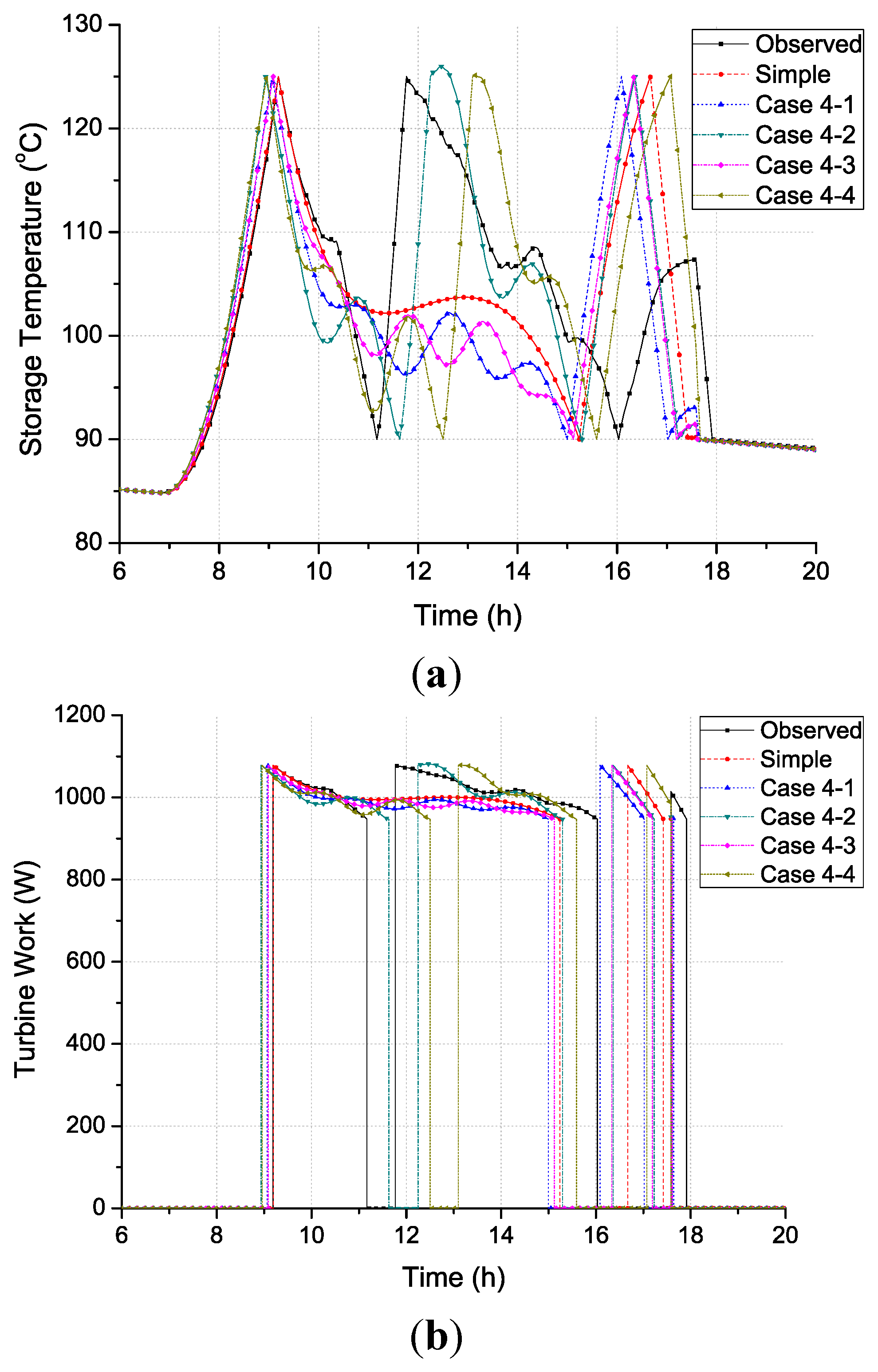
Figure 5 shows the simulation results for the thermal storage temperature and the shaft power. The results of storage temperature obtained both using the actual weather data and as predicted by the proposed model exhibit large variations and local overshoots, while the storage temperature predicted by the simple sky model shows a smooth behavior with significantly less variation. Thus, the temperature and shaft power results show that the proposed model provides better system operation characterization, including operation mode changes, than the simple sky model. In all cases, the amount of daily total solar irradiances is the same; however, the operating characteristics are dramatically changed according to the shape of solar irradiance distributions. In Cases 4-2 and Case 4-4, the system is turned off around noon, while in Cases 4-1 and 4-3, the model is not turned off, as an illustration of simple cases.
Table 3 lists the daily work total and its differences compared with the results of the observed data. In Case 4-4, weather variability does not match the observation when clouds appear, which results in different operating characteristics and the largest difference in daily work total. The case study results show that the proposed model does not perfectly express the actual observed weather condition and its system responses. However, it is possible to test a variety of weather conditions according to the study object.
Figure 5.
(a) Thermal storage temperature and (b) shaft power for the actual weather conditions, the simple sky model and the proposed model.
Figure 5.
(a) Thermal storage temperature and (b) shaft power for the actual weather conditions, the simple sky model and the proposed model.
Table 3.
Daily work total and its differences between the results of observed data and the others.
Table 3.
Daily work total and its differences between the results of observed data and the others.
| Parameters | Observed | Simple | Case 4-1 | Case 4-2 | Case 4-3 | Case 4-4 |
|---|
| Work Total (kWh) | 6.68 | 6.81 | 6.88 | 6.71 | 6.89 | 6.89 |
| Difference (%) | 0.00 | 1.92 | 2.93 | 0.43 | 3.04 | 3.04 |


