Stability Analysis for Li-Ion Battery Model Parameters and State of Charge Estimation by Measurement Uncertainty Consideration

Abstract

Accurate estimation of model parameters and state of charge (SoC) is crucial for the lithium-ion battery management system (BMS). In this paper, the stability of the model parameters and SoC estimation under measurement uncertainty is evaluated by three different factors: (i) sampling periods of 1/0.5/0.1 s; (ii) current sensor precisions of ±5/±50/±500 mA; and (iii) voltage sensor precisions of ±1/±2.5/±5 mV. Firstly, the numerical model stability analysis and parametric sensitivity analysis for battery model parameters are conducted under sampling frequency of 1–50 Hz. The perturbation analysis is theoretically performed of current/voltage measurement uncertainty on model parameter variation. Secondly, the impact of three different factors on the model parameters and SoC estimation was evaluated with the federal urban driving sequence (FUDS) profile. The bias correction recursive least square (CRLS) and adaptive extended Kalman filter (AEKF) algorithm were adopted to estimate the model parameters and SoC jointly. Finally, the simulation results were compared and some insightful findings were concluded. For the given battery model and parameter estimation algorithm, the sampling period, and current/voltage sampling accuracy presented a non-negligible effect on the estimation results of model parameters. This research revealed the influence of the measurement uncertainty on the model parameter estimation, which will provide the guidelines to select a reasonable sampling period and the current/voltage sensor sampling precisions in engineering applications.

1. Introduction

The lithium-ion battery has been widely utilized as a promising power source of hybrid-electric vehicles (HEVs) and pure electric vehicles (EVs) for its high energy and power density, no memory effect, and slow rate of self-discharge. Reduced safety hazards and an efficient Li-ion battery system can be achieved by developing an advanced battery management system (BMS). The model parameters and state of charge (SoC) are two critical indicators for an efficient BMS to operate the battery system safely and extend the cell life longevity.

1.1. Literature Review

Many studies have been performed in literature about the battery model parameters and SoC estimation. According to their highlights, these works can be classified around four categories: (I) operation environments; (II) varied aging states; (III) modeling and algorithm error; and (IV) measurement uncertainty.

In Class I, He et al. [1] realized the influence different charging and discharging rates had on the cell capacity. They formulated the coulombic efficiency that related with the current rates (1/3C–3C) and flowing direction to achieve a more accurate SoC estimation. To improve the accuracy of the battery model further, the authors He et al. [2] and Xing et al. [3] considered the temperature effect with the range of −20–60 °C and 0–40 °C. In their research, the coulombic efficiency was expressed as the polynomial equation of temperature. Wang et al. [4] considered the current rates and temperature effect together to correct the coulombic efficiency by creating a table to achieve more precise estimation of SoC and energy. In contrast, Liu et al. [5] addressed this issue by using the back-propagation neural network (BPNN) model to manage the current rate and temperature effect, and their simulation results also presented great performance. In Class II, the authors [6,7] analyzed the aging effect in the SoC estimation for lithium-ion polymer battery (LiPB) by two methods: first, the cell nominal capacity was re-modified according to the actual health environments; second, the cell’s open circuit voltage (OCV) was re-expressed as a second order polynomial equation, which is related with the SoC and modified cell capacity. Based on the recursive least square (RLS) and adaptive Kalman filter algorithm, the SoC estimation could be maintained with high accuracy. Dai et al. [8] applied the SoC estimation on a Li-ion battery pack of multiple inconsistent cells with the averaged cell model. Then they attempted to estimate the SoC for each individual cell, and the simulation results indicated good performance for the model and algorithm. Zhong et al. [9] analyzed the difference between the cells and the impact of balance control to minimize the cell capacity variation. The battery pack in serial and parallel connections and the passive balance control effect were considered to evaluate the impact of cell uniformity and inconsistency.

In Class III of the modeling and algorithm error, the battery model should first be established. In general, the battery model consists of model parameters and OCV in two parts. The two major factors of parameters uncertainty in varying aging and temperature effects have been reviewed previously. This review will address the OCV variation and SoC estimation algorithm uncertainty under different environments. Liu et al. [10] conducted the OCV test from 0 °C to 45 °C, and compared the OCV variation with temperature effect by creating a table. Hu et al. [11] provided the OCV value for lithium nickel-manganese-cobalt oxide (LiNMC) and lithium iron phosphate (LiFePO₄) cell by a series of polynomial functions with variables of temperature and SoC. Xiong et al. [12] presented the OCV functions for four different kinds of chemistry cells, such as carbon/lithium manganese oxide (C/LMO), lithium titanate oxide/nickel-manganese-cobalt-oxide (LTO/NMC), carbon/NMC (C/NMC) and carbon/lithium iron phosphate (C/LFP). Their simulation showed that the adaptive extended Kalman filter (AEKF) based SoC estimation method is suitable for multiple kinds of cells and obtained good estimation results with a maximum error being less than 3%. About the adaptive algorithm for SoC estimation, the extended Kalman filter (EKF) algorithm is firstly applied to the lithium ion polymer battery by Plett [13,14,15] in the work. Afterward, more extensive studies were conducted to assess the effect of the initial SoC creation, process covariance R_k, and measurement covariance Q_k [16,17]. To overcome the uncertainty of measurement noise covariance and initial SoC creation, the unscented Kalman filter [2,18,19], the particle filter [9,20,21], the AEKF [1,7,12], and the adaptive observer [22,23] techniques are proposed for SoC estimation. In Class IV, the measurement uncertainty remains an emerging research field according to our knowledge. Liu et al. [10] analyzed the current measurement with drift noise effect on SoC estimation by a dual-particle-filter estimator. In their study, the drift current was considered as an undetermined static parameter in the battery model to eliminate the drift current effect. Xia et al. [24] conducted the SoC estimation under the measurement error of both 2.5% voltage noise and 5% current noise. The results showed the SoC estimation error would not exceed 4.5%. However, as stated in [25], the current sensors have a certain grade of measurement accuracy and resolution. The amplifier circuit also exhibited some accuracy issues with the adaptation of resistors, capacitors and power lines. The micro-control-unit (MCU) involved the rounding errors in the process of analogue to digital (A/D) conversion and calculation. The current signal with harmonics also caused measurement errors during the sampling process with the MCU. All these noises and uncertainties in the measurement loop will generate errors for model parameters and SoC estimation. The detailed information is summarized and listed in the following Table 1.

Table 1. Factors influencing on the model parameters and state of charge (SoC) estimation.

Attribution	Item in detail	Reference
I. Operation environments	I.1. Current direction and rates	[1,2,3,4,5]
	I.2. Temperature effect
II. Varied aging states	II.1. Battery capacity loss during aging cannot be counted in the SoC calculation	[6,7]
	II.2. Cell inconsistency	[8,9]
	II.3. Self-discharging cannot be counted for by the SoC algorithm	unknown
III. Modeling and algorithm error	III.1. Parameters uncertainty due to varying aging	[6,7]
	III.2. Parameters uncertainty due to varying temperature	[2,3,4,5]
	III.3. OCV uncertainty due to varying aging	[6]
	III.4. OCV uncertainty due to varying temperature	[10]
	III.5. OCV uncertainty due to battery types	[11]
	III.6. Different sampling rate Ts	unknown
	III.7. Battery initial SoC remains unknown	[16]
	III.8. Different noise covariance Rk, Qk
	III.9. Different model accuracy and adaptive algorithms	[1]
IV. Measurement uncertainty	IV.1. Current measurement with drift noise	[10]
	IV.2. Different sampling rate Ts	unknown
	IV.3. Current sensor with different resolution	unknown
	IV.4. Current sensor with different precision	[24]
	IV.5. Voltage sensor with different resolution	unknown
	IV.6. Voltage sensor with different precision	[24]
	IV.7. Loading/excitation profile dependence	unknown

Table 1. Factors influencing on the model parameters and state of charge (SoC) estimation.

Attribution	Item in detail	Reference
I. Operation environments	I.1. Current direction and rates	[1,2,3,4,5]
	I.2. Temperature effect
II. Varied aging states	II.1. Battery capacity loss during aging cannot be counted in the SoC calculation	[6,7]
	II.2. Cell inconsistency	[8,9]
	II.3. Self-discharging cannot be counted for by the SoC algorithm	unknown
III. Modeling and algorithm error	III.1. Parameters uncertainty due to varying aging	[6,7]
	III.2. Parameters uncertainty due to varying temperature	[2,3,4,5]
	III.3. OCV uncertainty due to varying aging	[6]
	III.4. OCV uncertainty due to varying temperature	[10]
	III.5. OCV uncertainty due to battery types	[11]
	III.6. Different sampling rate Ts	unknown
	III.7. Battery initial SoC remains unknown	[16]
	III.8. Different noise covariance Rk, Qk
	III.9. Different model accuracy and adaptive algorithms	[1]
IV. Measurement uncertainty	IV.1. Current measurement with drift noise	[10]
	IV.2. Different sampling rate Ts	unknown
	IV.3. Current sensor with different resolution	unknown
	IV.4. Current sensor with different precision	[24]
	IV.5. Voltage sensor with different resolution	unknown
	IV.6. Voltage sensor with different precision	[24]
	IV.7. Loading/excitation profile dependence	unknown

1.2. Motivations and Contributions

The measuring system will inevitably bring in uncertainty and errors between measured signal and true signal from sampling aliases, conversion loss, and rounding calculation solutions. In this paper, the key innovation and contribution was to evaluate the effects of the measurement uncertainty on battery model parameter and SoC estimation both in theory and experiments. Different from other research, the measurement uncertainty is assumed from three different factors: (a) sampling periods of 1/0.5/0.1 s; (b) current sensor precisions of ±5/±50/±500 mA; and (c) voltage sensor precisions of ±1/±2.5/±5 mV. Afterward, the perturbation analysis of current and voltage measurement uncertainties, model stability analysis and parametric sensitivity analysis of model parameters were conducted respectively. The analytical result and conclusion provided guidelines that an engineer could use to choose the optimal sampling periods and current/voltage sensor precisions for improved estimation accuracy of model parameters and SoC.

1.3. Organization of the Paper

This paper will be organized as follows. In Section 2, the discrete battery model is given and the perturbation analysis of current/voltage measurement uncertainty, model stability analysis and parametric sensitivity analysis are conducted. In Section 3, the AEKF algorithm was adopted for the SoC estimation based on the auto regressive exogenous (ARX) battery model. In Section 4, the experiment setup is established, and the measured OCV-SoC curve is presented. In Section 5, the simulations were implemented upon three different factors. Then, the comparison is performed to analyze the weighted importance of factors on parameter and SoC estimation. Finally, the paper ends with a concluding remark.

2. Battery Model Analysis and Parameter Estimation

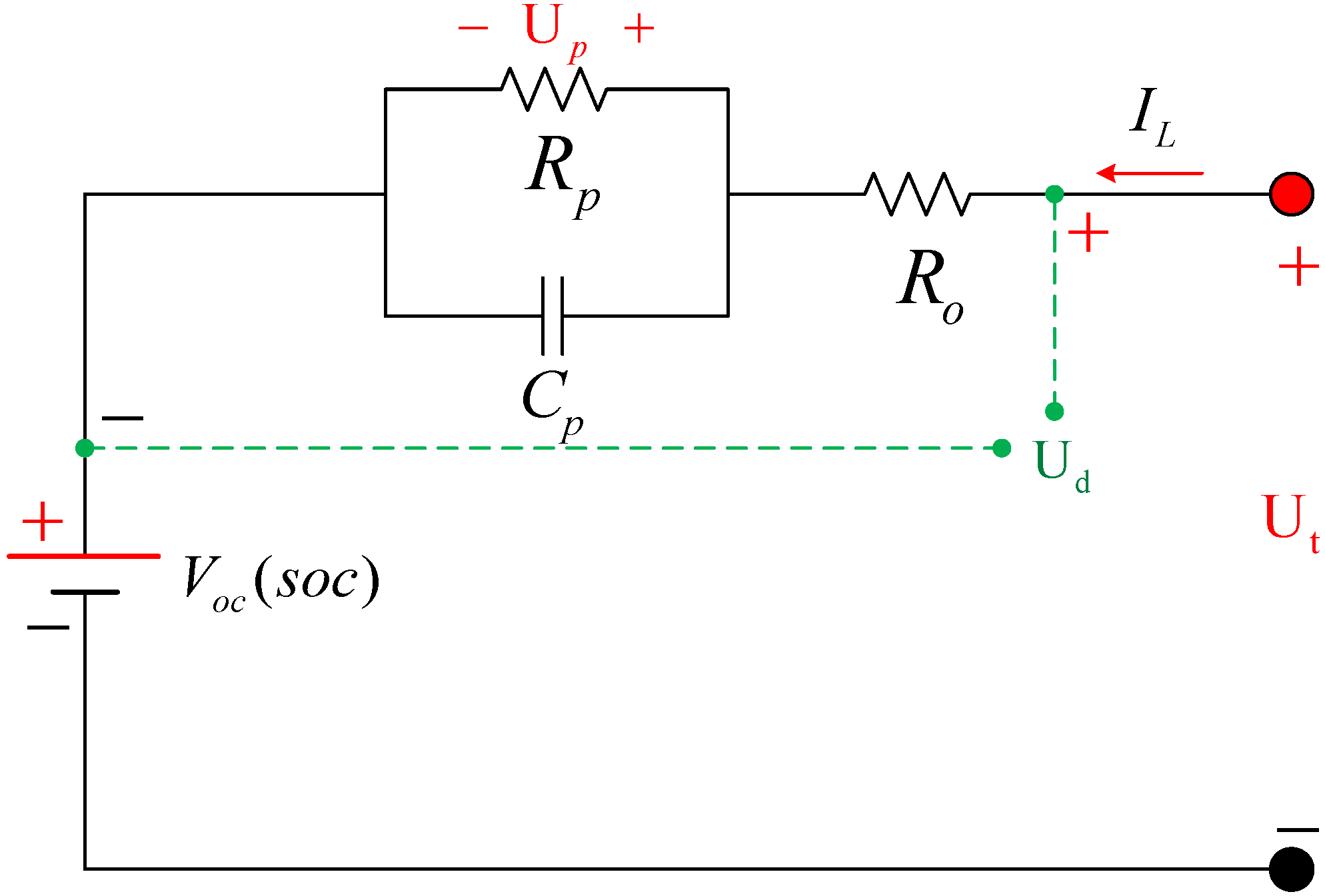
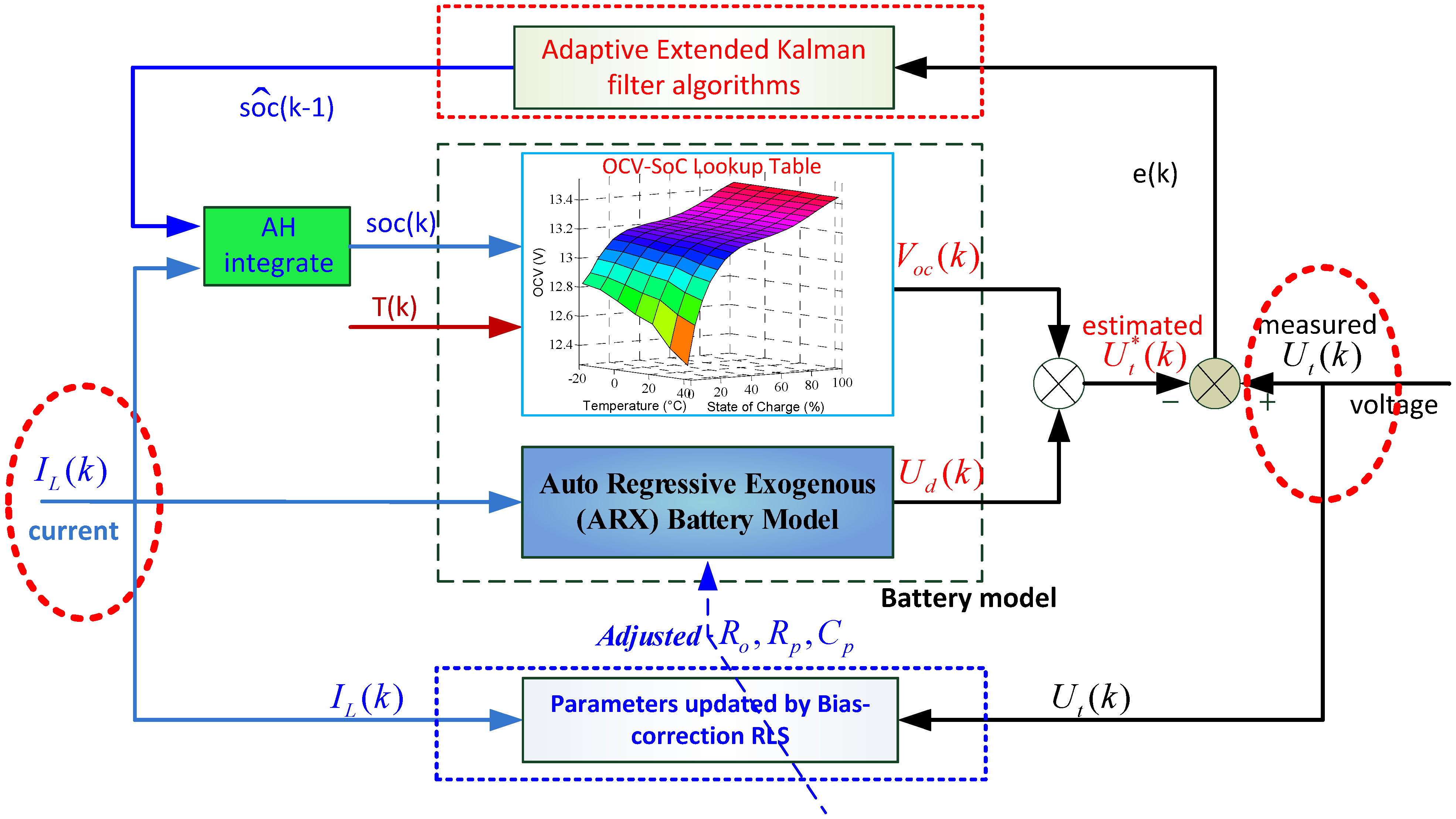
2.1. Auto Regressive Exogenous (ARX) Battery Model

As shown in Figure 1, the equivalent circuit model is employed to simulate the cell dynamic performance. It consists of an ohmic resistor R_o, open circuit voltage $V_{\text{oc}}\left(\text{SoC}\right)$ and one R_pC_p network connected in series. The resistor R_o represents the cell internal resistance. The R_pC_p network describes the electrochemical polarization dynamics. The electrical behavior of the lithium-ion battery can be expressed by the following equation:

$$\{\begin{array}{l}{\dot{U}}_{\text{p}}=-\frac{1}{C_{\text{p}}{R}_{\text{p}}}{U}_{\text{p}}+\frac{1}{C_{\text{p}}}{I}_L\\ U_{\text{t}}=V_{\text{oc}}\text{+}{U}_{\text{p}}\text{+}{R}_{\text{o}}{I}_{\text{L}}\end{array}$$

(1)

where U_p indicates the polarization voltage across the RC network. I_L stands for the applied current and U_t stands for the terminal voltage. SoC is defined by current integration as:

$$SoC(k+1)=SoC(k)+\frac{{\text{η}}_{\mathrm{i}}{T}_{\text{s}}}{Q_{\text{n}}}\cdot I_{\text{L}}(k)$$

(2)

where η_i is the coulombic efficiency, which is related with the current flow direction and magnitude, temperature, and the degradation/aging status. Herein, as the coulombic efficiency is not the priority in this research, the value of η_i is assumed to be 1. T_s is the sampling interval, and Q_n is the nominal capacity.

Figure 1. The schematic diagram of the equivalent circuit model for lithium-ion battery.

Figure 1. The schematic diagram of the equivalent circuit model for lithium-ion battery.

A bilinear transformation method $s=\frac{2}{T_{\text{s}}}\frac{1-z^{-1}}{1+z^{-1}}$ is employed to discrete the battery model into z domain for a given sampling interval, and the discrete transfer function is given as Equation (3):

$$G(z^{-1})=\frac{b_0+b_1{z}^{-1}}{1+a_1{z}^{-1}}$$

(3)

With the model parameters [a₁, b₀, b₁] equated as:

$$a_1=-\frac{T_{\text{s}}-2R_{\text{p}}{C}_{\text{p}}}{T_{\text{s}}+2R_{\text{p}}{C}_{\text{p}}};b_0=\frac{R_{\text{o}}{T}_{\text{s}}+R_{\text{p}}{T}_{\text{s}}+2R_{\text{o}}{R}_{\text{p}}{C}_{\text{p}}}{T_{\text{s}}+2R_{\text{p}}{C}_{\text{p}}};b_1=\frac{R_{\text{o}}{T}_{\text{s}}+R_{\text{p}}{T}_{\text{s}}-2R_{\text{o}}{R}_{\text{p}}{C}_{\text{p}}}{T_{\text{s}}+2R_{\text{p}}{C}_{\text{p}}}$$

(4)

It can be found the model parameters [a₁, b₀, b₁] are not only subjected to R_o, R_p, C_p, but also related to the sampling period T_s. R_o, R_p, and C_p can be solved based on the inverse equations of a₁, b₀ and b₁:

$$R_{\text{o}}=\frac{b_0-b_1}{1+a_1};R_{\text{p}}=\frac{2\left(a_1{b}_0+b_1\right)}{1-a_1^2};C_{\text{p}}=\frac{T{\left(1+a_1\right)}^2}{4\left(a_1{b}_0+b_1\right)}$$

(5)

After discretization, Equation (3) can be rewritten in the form of ARX as follows:

$$U_{\text{d}}(k)=a_1{U}_{\text{d}}(k-1)+b_0{I}_{\text{L}}(k)+b_1{I}_{\text{L}}(k-1)$$

(6)

where k is the time point, k = 1,2,3,…. N. Since U_d = U_t − V_oc:

$$\begin{array}{ll}{U}_{\text{t}}(k)& =\left[V_{\text{oc}}(k)-a_1{V}_{\text{oc}}(k-1)\right]+a_1{U}_{\text{t}}(k-1)+b_0{I}_{\text{L}}(k)+b_1{I}_{\text{L}}(k-1)\\ & \approx (1-a_1)V_{\text{oc}}(k-1)+a_1{U}_{\text{t}}(k-1)+b_0{I}_{\text{L}}(k)+b_1{I}_{\text{L}}(k-1)\end{array}$$

(7)

The information vector is defined as the following $\text{Φ}\left(k\right)=\left[\begin{array}{cc}\begin{array}{ccc}{U}_L\left(k-1\right)& I_L\left(k\right)& I_L\left(k-1\right)\end{array}& 1\end{array}\right]$ and the parameter vector is defined as $\text{Θ}\left(k\right)={\left[\begin{array}{cc}\begin{array}{ccc}{a}_1& b_0& b_1\end{array}& \left(1-a_1\right){\text{V}}_{\text{oc}}\end{array}\right]}^T$, then they can be combined as the following:

$$Y(k)=\text{Φ}(k)\cdot \text{Θ}(k)$$

(8)

The RLS algorithm [26] is an effective method for online parameter identification. As an improved algorithm, the bias correction recursive least square (CRLS) technique [27] is used in this paper. The basic idea of CRLS is to eliminate the estimation bias by adding a correction term in the RLS estimation algorithm. Therefore, the performance and numerical convergence of the algorithm can be prompted to a higher level. The detailed implementation of CRLS algorithm could refer to our previous work [28].

2.2. Perturbation Analysis of Measurement Uncertainty

In the literature, there are many adaptive methods for parameter identification, such as RLS, EKF, and adaptive observers. All these methods can give the recursive-identified value for model parameters. However, they cannot tell the parameter variation under current and voltage measurement uncertainty. In this section, the parameter variation is theoretically analyzed under the perturbation of current/voltage measurement uncertainty. Based on above Equations (4) and (7), the formula of parameters (R_o, R_p, C_p) can be deducted as follows:

$$R_{\text{o}}=\frac{\left(T_{\text{s}}+2R_{\text{p}}{C}_{\text{p}}\right)U_{\text{t}}\left(k\right)+\left(T_{\text{s}}-2R_{\mathrm{p}}{C}_{\text{p}}\right)U_{\text{t}}\left(k-1\right)-2T_{\text{s}}\cdot V_{\text{oc}}(\mathrm{k}-1)-\left(R_{\text{p}}\cdot T_{\text{s}}\right)\left(I_{\text{L}}\left(k\right)+I_{\text{L}}\left(k-1\right)\right)}{\left(T_{\text{s}}+2R_{\text{p}}{C}_{\text{p}}\right)I_{\text{L}}\left(k\right)+\left(T_{\text{s}}-2R_{\text{p}}{C}_{\text{p}}\right)I_{\text{L}}\left(k-1\right)}$$

(9)

$$R_{\text{p}}=\frac{T_{\text{s}}\cdot \left(U_{\text{t}}\left(k\right)+U_{\text{t}}\left(k-1\right)-2V_{\text{oc}}\left(k-1\right)\right)-R_{\text{o}}{T}_{\text{s}}\cdot \left(I_{\text{L}}\left(k\right)+I_{\text{L}}\left(k-1\right)\right)}{-2C_{\text{p}}\cdot \left(U_{\text{t}}\left(k\right)-U_{\text{t}}\left(k-1\right)\right)+\left(T_{\text{s}}+2R_{\text{p}}{C}_{\text{p}}\right)I_{\text{L}}\left(k\right)+\left(T_{\text{s}}-2R_{\text{p}}{C}_{\text{p}}\right)I_{\text{L}}\left(k-1\right)}$$

(10)

$$C_{\text{p}}=\frac{-T_{\text{s}}\cdot \left(U_{\text{t}}\left(k\right)+U_{\text{t}}\left(k-1\right)-2V_{\text{oc}}\left(k-1\right)\right)+\left(R_{\text{o}}+R_{\text{p}}\right)T_{\text{s}}\cdot \left(I_{\text{L}}\left(k\right)+I_{\text{L}}\left(k-1\right)\right)}{2R_{\text{p}}\cdot \left(U_{\text{t}}\left(k\right)-U_{\text{t}}\left(k-1\right)\right)-2R_{\text{o}}{R}_{\text{p}}\cdot \left(I_{\text{L}}\left(k\right)-I_{\text{L}}\left(k-1\right)\right)}$$

(11)

These expressions can be used to analyze the impact of measurement errors (δI_L, δU_t) on the model parameters (R_o, R_p, C_p). Let’s take the ohmic resistance R_o, for an example, to illustrate how the current sensor error δI_L affects the estimated results of R_o. By incorporating the current error δI_L, the new modified current (I_L + δI_L) will replace the I_L in Equation (9) to achieve the new estimated $R_{\text{o}}^{\prime }$. Then, the relative error of R_o can be defined as:

$$\text{ε}=\left|\frac{R_{\text{o}}^{\prime }-R_{\text{o}}}{R_{\text{o}}}\right|\times 100\%$$

(12)

By this method, the effect of current sensor error δI_L on the parameter variation can be analyzed. Since the battery system is time-varying, the pulse current excitation (1.0C, 30 s) is chosen as a typical profile. In this research, the current sensor error δI_L is assumed as ±5/±50/±500 mA. The calculation result is listed in Figure 2a–c. Similarly, the voltage sensor error δU_t (±1/±2.5/±5 mV) effect on the parameter variation can be assessed in Figure 2d–f).

Figure 2. Relative errors of model parameters: (a) R_o, (b) R_p, (c) C_p under current noises; and (d) R_o, (e) R_p, (f) C_p under voltage noises.

Figure 2. Relative errors of model parameters: (a) R_o, (b) R_p, (c) C_p under current noises; and (d) R_o, (e) R_p, (f) C_p under voltage noises.

Seen from Figure 2, the ohmic resistance R_o is more robust than the R_p and C_p. As the current noise and voltage noise enhanced, the relative error of parameters enlarged. The R_p and C_p are used to express the battery dynamic performance, and at the beginning of pulse current excitation, the load current flows mostly upon the capacitor. Therefore, the relative error of capacitor C_p is smaller at the beginning. In contrast, the relative error of resistance R_p is much larger at the beginning. The minimum values of relative error of model parameters (R_o, R_p, C_p) under current/voltage noises are summarized in Table 2.

Table 2. Minimum values of relative error of model parameters (R_o, R_p, C_p) under current/voltage noises.

Item	Magnitude of noise	Parameter relative error (%) @ 0.2C			Parameter relative error (%) @ 1.0C
		Ro	Rp	Cp	Ro	Rp	Cp
Current noise	δIL = ±5 mA	0.0625	0.1513	0.1411	0.0125	0.0303	0.0282
	δIL = ±50 mA	0.6224	1.5058	1.4111	0.1249	0.3024	0.2822
	δIL = ±500 mA	6.000	14.407	14.111	1.2397	2.9966	2.8223
Voltage noise	δUt = ±1 mV	4.1667	8.5613	9.2046	0.8333	1.7123	1.8815
	δUt = ±2.5 mV	10.416	21.403	23.518	2.0833	4.2806	4.7038
	δUt = ±5 mV	20.833	42.806	47.037	4.1667	8.5613	9.4076

Table 2. Minimum values of relative error of model parameters (R_o, R_p, C_p) under current/voltage noises.

Item	Magnitude of noise	Parameter relative error (%) @ 0.2C			Parameter relative error (%) @ 1.0C
		Ro	Rp	Cp	Ro	Rp	Cp
Current noise	δIL = ±5 mA	0.0625	0.1513	0.1411	0.0125	0.0303	0.0282
	δIL = ±50 mA	0.6224	1.5058	1.4111	0.1249	0.3024	0.2822
	δIL = ±500 mA	6.000	14.407	14.111	1.2397	2.9966	2.8223
Voltage noise	δUt = ±1 mV	4.1667	8.5613	9.2046	0.8333	1.7123	1.8815
	δUt = ±2.5 mV	10.416	21.403	23.518	2.0833	4.2806	4.7038
	δUt = ±5 mV	20.833	42.806	47.037	4.1667	8.5613	9.4076

2.3. Model Stability Analysis

Model stability is critical to indicate the model stable and robust level under external perturbation. As the model stability is increased, the model output will be much stable; meanwhile the identification of model parameters will be much easier. The two key factors (poles and zeros) will be used to reveal the model stability level in a quantifiable form. A detailed process for poles and zeros calculation is in the author’s previous work [28].

To assess the model stability, the battery parameters are assumed as R_o = 0.002 Ω; R_p = 0.001 Ω; C_p = 8000 F; T_s = 1 s, 0.5 s, 0.2 s, 0.1 s, 0.02 s, and the parameter sets [a₁, b₀, b₁] of the ARX model is calculated using Equation (4). Meanwhile, the model poles and zeros can be computed to present the model stability level and the result is listed in Table 3.

From Table 3, the poles and zeros of the system increased as T_s decreased, which reveals the model stability is degraded. According to the Lyapunov’s first stability criterion, the model stability will become much poorer as the eigenvalues of the ARX model get close to one. That is, perturbations caused by noise and unmodeled dynamics could significantly influence the accuracy of model parameter identification. To this point, the sampling rate should be lower (i.e., sampling period should be higher), to improve the model stability and the robustness of parameter identification. From an engineering viewpoint, it is recommended to restrict the eigenvalues within a range of 0–0.95. In other words, T_s should be larger than one threshold, such as T_s ≥ 0.5 s.

Table 3. Parameter variation and stability analysis for the auto regressive exogenous (ARX) model.

Sampling Ts (s)	Parameter variation			Stability analysis
	a1	b0	b1	Pole	Zero
1	0.88235	0.00205	−0.00170	0.88235	0.82857
0.5	0.93939	0.00203	−0.00184	0.93939	0.91044
0.2	0.97530	0.00201	−0.00193	0.97530	0.96319
0.1	0.98757	0.00200	−0.00196	0.98757	0.98142
0.02	0.99750	0.00200	−0.00199	0.99750	0.99625

Table 3. Parameter variation and stability analysis for the auto regressive exogenous (ARX) model.

Sampling Ts (s)	Parameter variation			Stability analysis
	a1	b0	b1	Pole	Zero
1	0.88235	0.00205	−0.00170	0.88235	0.82857
0.5	0.93939	0.00203	−0.00184	0.93939	0.91044
0.2	0.97530	0.00201	−0.00193	0.97530	0.96319
0.1	0.98757	0.00200	−0.00196	0.98757	0.98142
0.02	0.99750	0.00200	−0.00199	0.99750	0.99625

In another way, the sampling period T_s should be chosen modestly enough to capture the significant variation or critical events of Li-ion cell dynamics. In the viewpoint of hardware runtime, the sampling period T_s should be sufficient for the SoC calculation on the ECU platform with the discrete battery model, CRLS and AEKF algorithms. Therefore, the optimized time sampling period must be selected in a tradeoff way by considering the model stability, parametric sensitivity, system-sampling precision and the hardware runtime.

2.4. Parametric Sensitivity Analysis

In this research, the model parameters are identified online by CRLS. In other words, the variations of a₀, b₀, or b₁ will affect the model parameter set P of R_o, R_p, and C_p. The sensitivity of the model parameters to the changes in variable α (such as a₀, b₀, or b₁) is given by the partial differentiation of P(s) with respect to α and is denoted as:

$$S_{\text{α}}^P=\frac{\text{α}}{P}\cdot \frac{\partial P}{\partial \text{α}}$$

(13)

where P is the parameter set of R_o, R_p, and C_p as defined in Equation (5), and α is a₀, b₀, or b₁. To be specific [28]:

$$S_{\text{α}}^P=\left[\begin{array}{ccc}{S}_{a_1}^{R_o}& S_{b_0}^{R_o}& S_{b_1}^{R_o}\\ S_{a_1}^{R_p}& S_{b_0}^{R_p}& S_{b_1}^{R_p}\\ S_{a_1}^{C_p}& S_{b_0}^{C_p}& S_{b_1}^{C_p}\end{array}\right]$$

(14)

Based on the sensitivity equation, the parametric sensitivity has been calculated at four sampling periods (T_s = 1 s, 0.5 s, 0.1 s and 0.02 s), and the results are listed in Table 4.

Table 4. Parametric sensitivity analysis of the ARX model at four sample periods (T_s = 1/0.5/0.1/0.02 s).

Item	Sensitivity	a1	b0	b1
Sample @ Ts = 1 s	Ro	−0.4688	0.5469	0.4531
	Rp	23.4374	16.4062	−15.4062
	Cp	−15.4688	−16.4063	15.4063
Sample @ Ts = 0.5 s	Ro	−0.4844	0.5234	0.4766
	Rp	47.4687	32.4531	−31.4531
	Cp	−31.4844	−32.4531	31.4531
Sample @ Ts = 0.1 s	Ro	−0.4969	0.5047	0.4953
	Rp	239.4938	160.4906	−159.4906
	Cp	−159.4969	−160.4906	159.4906
Sample @ Ts = 0.02 s	Ro	−0.4994	0.5009	0.4991
	Rp	1199.5	800.4981	−799.4981
	Cp	−799.4994	−800.4981	799.4981

Table 4. Parametric sensitivity analysis of the ARX model at four sample periods (T_s = 1/0.5/0.1/0.02 s).

Item	Sensitivity	a1	b0	b1
Sample @ Ts = 1 s	Ro	−0.4688	0.5469	0.4531
	Rp	23.4374	16.4062	−15.4062
	Cp	−15.4688	−16.4063	15.4063
Sample @ Ts = 0.5 s	Ro	−0.4844	0.5234	0.4766
	Rp	47.4687	32.4531	−31.4531
	Cp	−31.4844	−32.4531	31.4531
Sample @ Ts = 0.1 s	Ro	−0.4969	0.5047	0.4953
	Rp	239.4938	160.4906	−159.4906
	Cp	−159.4969	−160.4906	159.4906
Sample @ Ts = 0.02 s	Ro	−0.4994	0.5009	0.4991
	Rp	1199.5	800.4981	−799.4981
	Cp	−799.4994	−800.4981	799.4981

First, the sensitivity of R_o with respect to parameters [a₀, b₀, b₁] was not great and always retained within [−0.45–0.54]. As the growth of T_s, the sensitivity of R_o on a₀, b₀, and b₁ became more uniform. This illustrated that R_o was much more robust and more easily identifiable regardless of the sampling period T_s. This characteristic was confirmed in our later simulation. Second, the sensitivity of R_p and C_p increased quasi-linearly as T_s decreased. Specifically, a small disturbance in a₀, b₀, and b₁ may cause large fluctuations in R_p and C_p when T_s is much smaller; therefore, this feature will also increase the difficulty for real-time parameter identification. In practice, it is suggested to limit T_s to be greater than a certain level to maintain good stability for parameter identification.

3. Adaptive Extended Kalman Filter Algorithm

In this section, the model states and parameters are estimated jointly based on real measurements of the current, voltage and temperature. In theory, the joint state and parameter estimation algorithm could provide a more accurate estimation result for battery model parameters and SoC. The general working principle of the joint estimation algorithm is displayed as Figure 3.

Figure 3. General diagram of the battery model parameters and SoC joint estimation with adaptive extended Kalman filter (AEKF) and correction recursive least square (CRLS) algorithms.

Figure 3. General diagram of the battery model parameters and SoC joint estimation with adaptive extended Kalman filter (AEKF) and correction recursive least square (CRLS) algorithms.

The AEKF [1,17,29] is an advanced method for system state estimation, especially when the system process and measurement noise are unknown. This algorithm can avoid the estimation error divergence effectively due to its robustness property. Furthermore, it can enhance the performance in the SoC estimation enormously.

Firstly, the general form of state space representation is presented as:

$$\begin{array}{l}{X}_{k+1}=f(X_k,u_k)+w_k\\ Y_k=g(X_k,u_k)+v_k\\ w_k\sim N(0,Q_k),v_k\sim N(0,R_k)\end{array}$$

(15)

where X_k is the model state, u_k is the model input, k is the time index, $f(\cdot )$ and $g(\cdot )$ indicate the process equation and output equation of the battery model, respectively, ω_k is a discrete time process white noise with a covariance matrix Q_k, whose initial value can be chosen by the state X_k properties. Similarly, υ_k is a discrete time measurement white noise with covariance matrix R_k, whose initial value can be determined according to the voltage sensor precision.

The battery model Equations (1) and (2) can be transformed as state space form:

$$\left[X_{k+1}\right]=\left[\begin{array}{c}SoC(k+1)\\ U_{\text{p}}(k+1)\end{array}\right]=\underset{\mathbf{f}(\cdot )}{\underbrace{\underset{{\widehat{A}}_k}{\underbrace{\left[\begin{array}{cc}1& 0\\ 0& \mathbf{exp}(\frac{-T_{\text{s}}}{R_{\text{p}}{C}_{\text{p}}})\end{array}\right]}}\underset{\mathrm{state}\mathbf{:}{X}_k}{\underbrace{\left[\begin{array}{c}SoC(k)\\ U_{\mathrm{p}}(k)\end{array}\right]}}+\left[\begin{array}{c}\frac{{\mathrm{\eta }}_{\text{i}}{T}_{\text{s}}}{Q_{\text{n}}}\\ R_{\text{p}}\left[1-\mathbf{exp}(\frac{-T_{\text{s}}}{R_{\text{p}}{C}_{\text{p}}})\right]\end{array}\right]\underset{\mathrm{input}\mathbf{:}{u}_k}{\underbrace{\left[I_{\mathrm{L}}(k)\right]}}}}$$

(16)

$$\left[Y_k\right]=\left[U_{\text{t}}(k)\right]=\underset{\mathbf{g}(\cdot )}{\underbrace{\underset{{\widehat{C}}_k}{\underbrace{\left[\begin{array}{cc}{\frac{\text{d}{V}_{\text{oc}}(SoC)}{\text{d}SoC}|}_{SoC=SoC(k)}& -1\end{array}\right]}}\underset{\mathrm{state}\mathbf{:}{X}_k}{\underbrace{\left[\begin{array}{c}SoC(k)\\ U_{\mathrm{p}}(k)\end{array}\right]}}+\left[-R_{\text{o}}\right]\underset{\mathrm{input}\mathbf{:}{u}_k}{\underbrace{\left[I_{\mathrm{L}}(k)\right]}}}}$$

(17)

After several iterations, the estimated model voltage will converge to the truly measured value; meanwhile, the estimated SoC will converge to the true or optimal value.

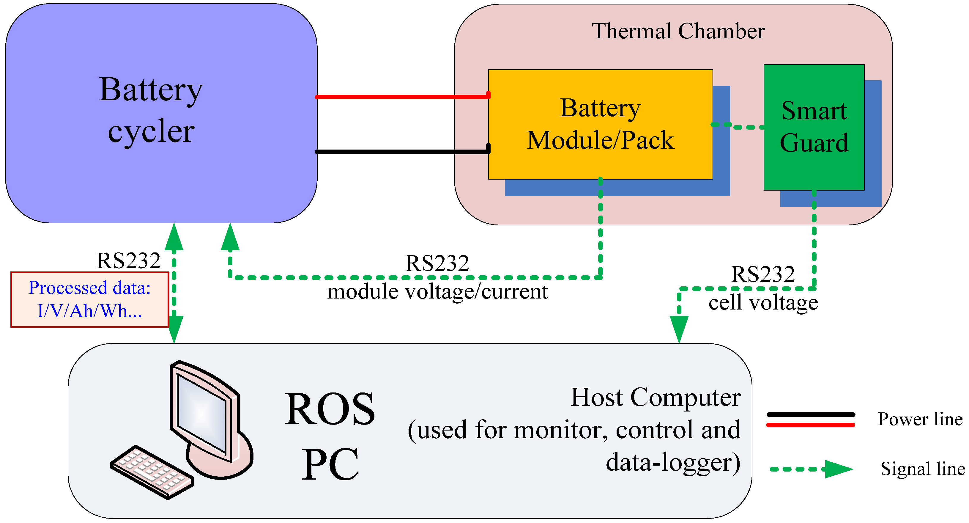
4. Experimental Setup

The test bench setup is shown as Figure 4. It consists of a battery cycler, a thermal chamber for temperature control, and a computer for script programming and data storage. The battery testing system is responsible for loading the battery module with maximum charging/discharging current of ±500 A. The measurement error of the current/voltage transducer inside the cycler is within 0.25%. The key specification of the LiFePO₄ cell is listed in Table 5.

Figure 4. Configuration of the battery test bench.

Figure 4. Configuration of the battery test bench.

Table 5. Main specifications of the test cell.

Type	Rated capacity	Rated energy	Maximum current	Rated voltage	Upper voltage	Lower voltage
LiFePO4	60 A h	192 W h	3C, 180 A	3.20 V	3.65 V	2.10 V

Table 5. Main specifications of the test cell.

Type	Rated capacity	Rated energy	Maximum current	Rated voltage	Upper voltage	Lower voltage
LiFePO4	60 A h	192 W h	3C, 180 A	3.20 V	3.65 V	2.10 V

The LiFePO₄ cell is cycled with the OCV test as stated in [16]. According to the emphasis and priority in this research, the averaged OCV is employed to simplify the hysteresis phenomena of the OCV under charging and discharging process. The computed result of averaged OCV is listed in Figure 5. The open circuit voltage V_oc(SoC) can be expressed by a polynomial function as:

$$V_{\text{oc}}\left(SoC\right)=K_0+K_1\cdot SoC+K_2\cdot So{C}^2+K_3\cdot So{C}^3+K_4\cdot So{C}^4$$

(18)

where K_i (i = 0, 1, …, 4) are the polynomial coefficients to fit the averaged OCV with respect to different SoC based on the least square techniques, and the specific values are 3.1292, 0.00025, 0.00085, 0.0421, 0.0076, respectively. By incremental capacity analysis (ICA), the dSoC/dOCV reaches its upper limit of 0.0145 at the voltage of about 3.280 V, which means the 1 mV estimated error of OCV will result in about 1.45% for SoC estimation bias.

Figure 5. (a) The open circuit voltage (OCV) test and (b) incremental capacity analysis (ICA) result at temperature 25 °C.

Figure 5. (a) The open circuit voltage (OCV) test and (b) incremental capacity analysis (ICA) result at temperature 25 °C.

5. Simulation and Discussion

In this section, the effects of measurement uncertainty on battery model parameters and SoC estimation is evaluated in the following three aspects: (i) sampling periods of 1/0.5/0.1 s; (ii) current sensor accuracy of ±5/±50/±500 mA; and (iii) voltage sensor accuracy of ±1/±2.5/±5 mV. In Section 5.4, the simulations of these three different scenarios are compared to evaluate the impact of each factor on the model parameters and SoC estimation. The federal urban driving sequence (FUDS) profile is a typical experiment cycle to assess the model and algorithm performance. In this research, the parameter sets Θ = [R_o, R_p, C_p] = [0.002, 0.001, 8000] is adopted as a baseline.

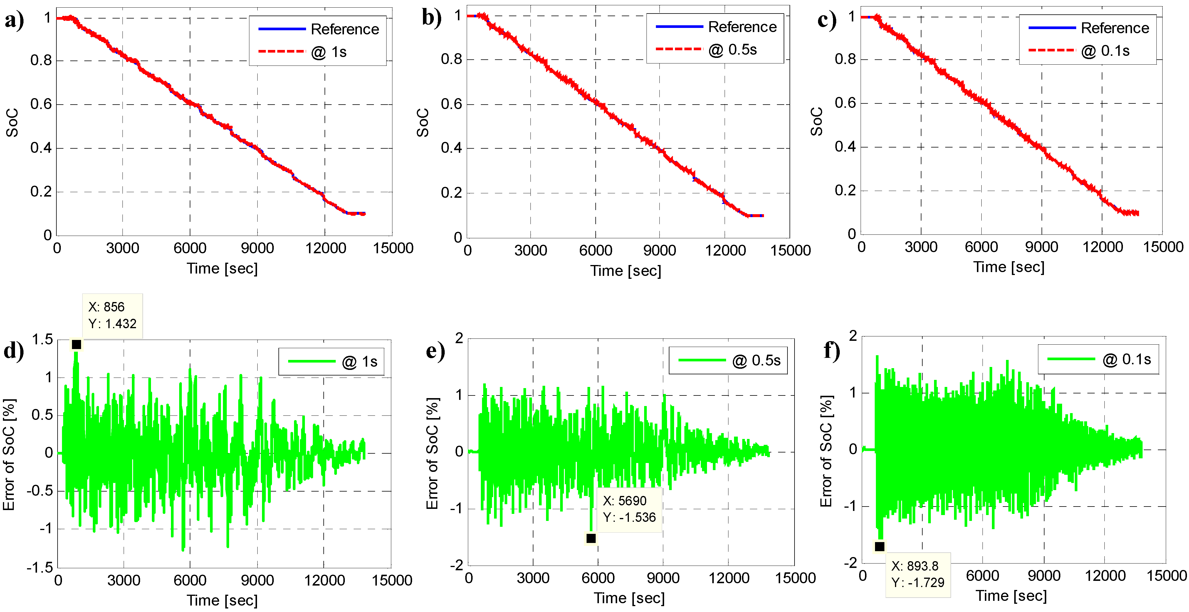
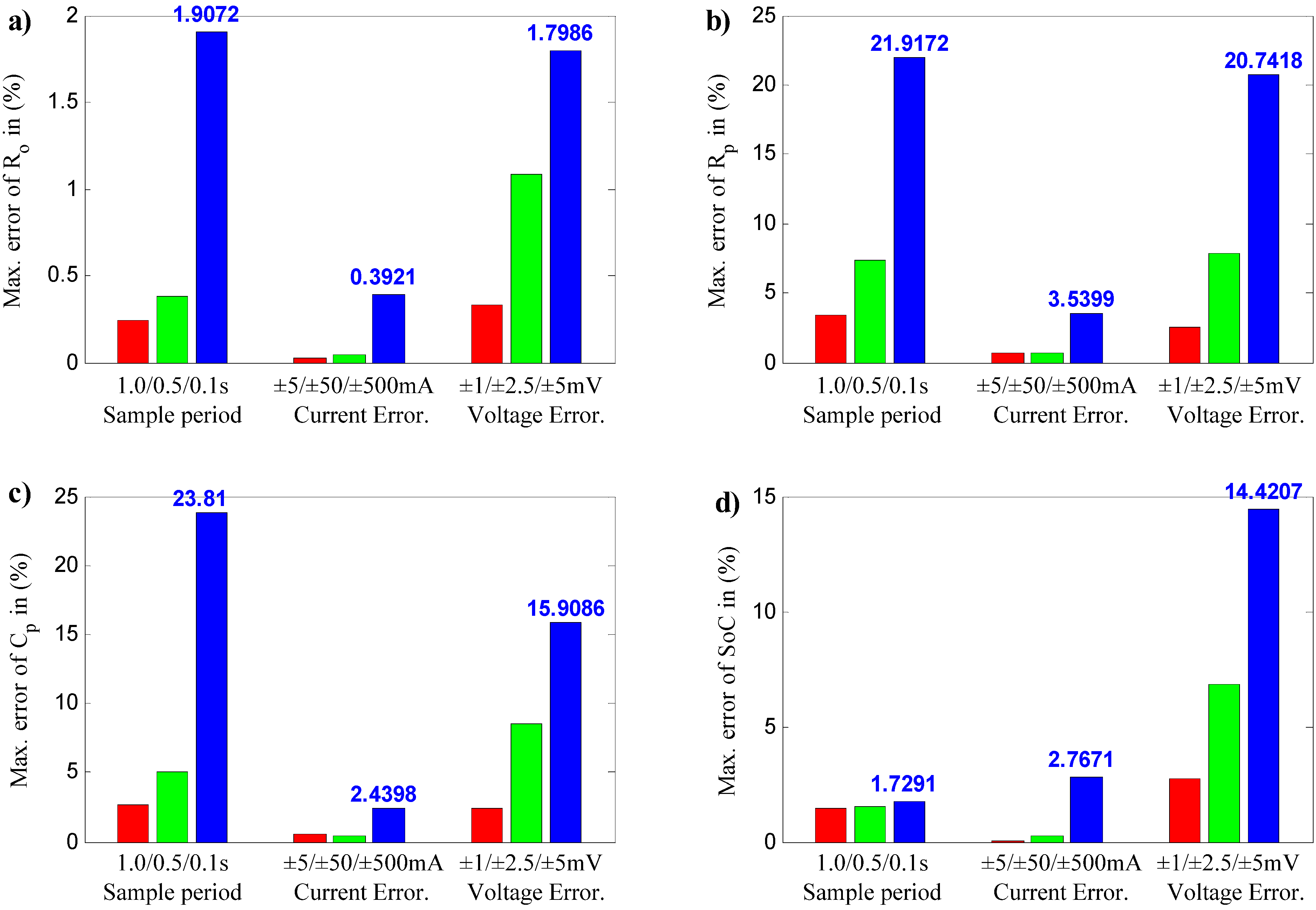
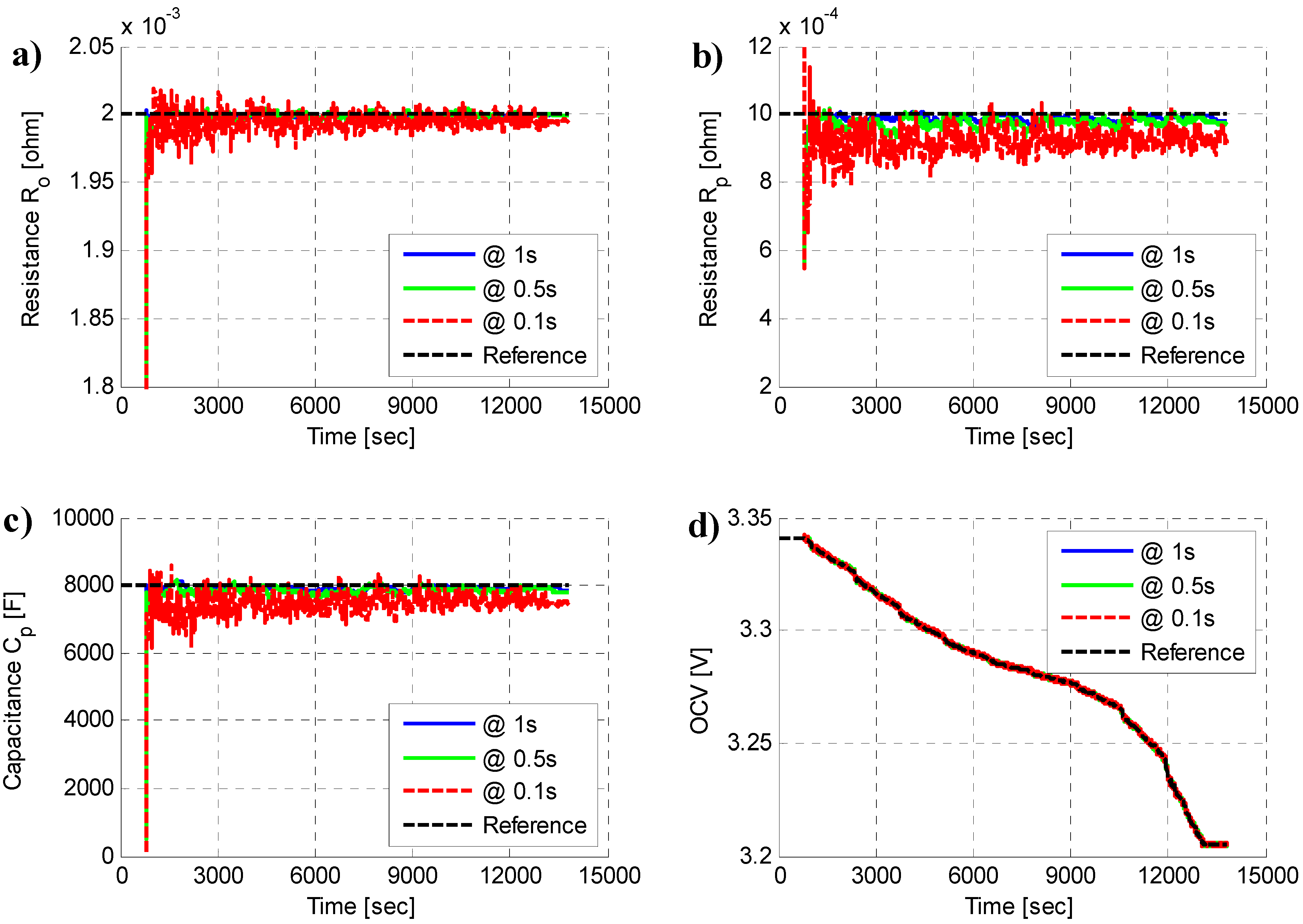
5.1. Sampling Period Effect

To evaluate the effect of the sampling periods on the battery model parameters and SoC estimation, three different sampling periods of 1/0.5/0.1 s are selected in the simulation with the CRLS and AEKF algorithm. The estimation results of the model parameters under the FUDS loading profiles are shown in Figure 6.

Figure 6. Estimated model parameters: (a) R_o, (b) R_p, (c) C_p and (d) OCV at the sampling periods of 1/0.5/0.1 s.

Figure 6. Estimated model parameters: (a) R_o, (b) R_p, (c) C_p and (d) OCV at the sampling periods of 1/0.5/0.1 s.

Figure 6a shows the estimated ohmic resistance R_o and the reference value. The maximum estimation error of R_o increases from 0.2408% to 1.9072% when the sampling rate increased from 1.0 s to 0.1 s. Figure 6b,c lists the estimated polarization resistance R_p and polarization capacitance C_p respectively. When the sampling period is 1 s, the maximum estimation errors of R_p and C_p are 3.3859% and 2.6605%. As the sampling period decreased to 0.1s, the maximum estimation errors of R_p and C_p increased hugely to 21.9172% and 23.81%. If three parameters (R_o, R_p and C_p) are compared together, it can be found the pair of R_p and C_p is much more sensitive to the noise. This conclusion can be verified by the previous model stability and parameter sensitivity analysis. As the sampling period declines from 1 s to 0.1 s, the model stability will degrade, and the parameter sensitivity will be intensified, which means the perturbation to the model parameters will be enhanced under the same noise excitation. Finally, the estimated OCV is plotted in Figure 6d. It reveals that the maximum estimation error of OCV remains nearly the same level. In other words, the sample period exhibits slighter effect on the OCV estimation.

Figure 7 is the estimation results of SoC and SoC error for three different sampling rates under the FUDS loading profiles. From Figure 7, we find that the SoC estimation errors for three different sampling rates are 1.432%, 1.536% and 1.729%. These results reveal that the effect of sampling rate on the SoC estimation accuracy is not significant. Through the comparison, it can infer that the sampling rate has more influence on the model parameters estimation than the SoC estimation. The statistical error analysis of model parameters and SoC, such as maximum error and root-mean-square error (RMSE) is shown in Table 6.

Figure 7. SoC estimation results at the sampling periods of (a) 1 s, (b) 0.5 s, (c) 0.1 s; and the SoC error at the sampling periods of (d) 1 s, (e) 0.5 s, (f) 0.1 s.

Figure 7. SoC estimation results at the sampling periods of (a) 1 s, (b) 0.5 s, (c) 0.1 s; and the SoC error at the sampling periods of (d) 1 s, (e) 0.5 s, (f) 0.1 s.

Table 6. The statistical error analysis of model parameters and SoC estimation error. RMSE: root-mean-square error.

Item	Sample @ 1.0s				Sample @ 0.5s				Sample @ 0.1s
Parameters	Ro	Rp	Cp	SoC	Ro	Rp	Cp	SoC	Ro	Rp	Cp	SoC
Maximum error (%)	0.24	3.38	2.66	1.43	0.38	7.33	5.09	1.53	1.90	21.9	23.8	1.72
RMSE (%)	0.06	1.34	1.23	0.33	0.11	2.55	2.10	0.34	0.38	8.39	7.31	0.36

Table 6. The statistical error analysis of model parameters and SoC estimation error. RMSE: root-mean-square error.

Item	Sample @ 1.0s				Sample @ 0.5s				Sample @ 0.1s
Parameters	Ro	Rp	Cp	SoC	Ro	Rp	Cp	SoC	Ro	Rp	Cp	SoC
Maximum error (%)	0.24	3.38	2.66	1.43	0.38	7.33	5.09	1.53	1.90	21.9	23.8	1.72
RMSE (%)	0.06	1.34	1.23	0.33	0.11	2.55	2.10	0.34	0.38	8.39	7.31	0.36

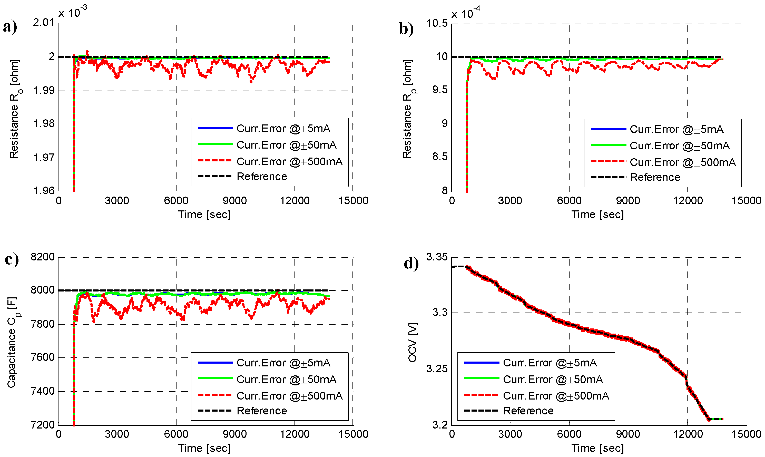
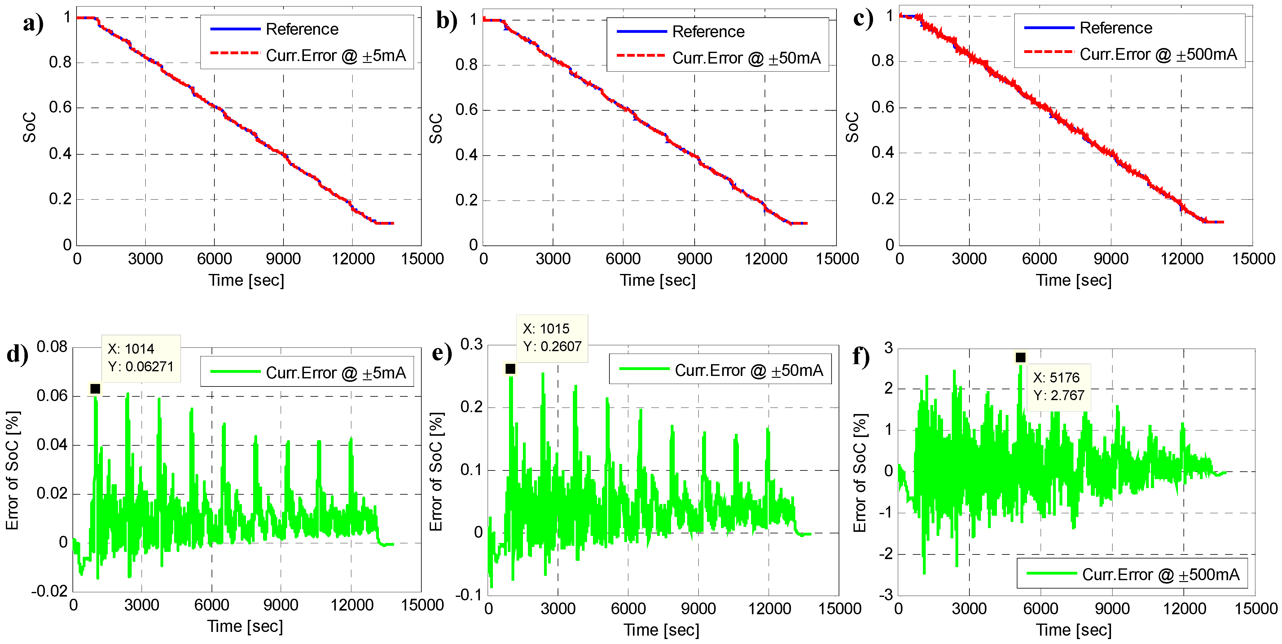
5.2. Current Sensor Accuracy Effect

In the engineering application, the accuracy of the current sensor/transformer is divided into six grades of 0.1, 0.2, 0.5, 1, 3, 5, according to China’s national standards GB 1208-1997. The number listed here indicates that the accuracy of the current sensor with the unit of the percentage. To be instinctive, some typical current transducers with detailed specification [30,31] are collected in the following Table 7. From the table, it can be found that the sensor accuracy is varied from ±50 mA to ±500 mA for different kinds of current transducers.

Table 7. The accuracy information comparison of three typical current sensors.

Company and product name	LEM DHAB S/25 (Geneva, Switzerland)	LEM LA100-P (Geneva, Switzerland)	Allegro, ACS758 LCB-100B-PSF-T (Worcester, MA, USA)
Transducer type	Open loop	Closed loop	Closed loop
Supply voltage	5 V	5 V	3.3 V or 5 V
Primary current Ip	±25 A for ch1; ±200 A for ch2	±100 A	±100 A
Output voltage Vsn	0.25–4.75 V	-	Vref ±2 V
Overall accuracy @Ip, T = 25 °C	±4%, ±500 mA	±0.45%, ±50 mA	±2.4%, ±150 mA
Linearity error	<±1%	<±0.15%	<±1.25%
Operation temperance	−40.125 °C	−40.85 °C	−40.150 °C
Response time	<25 ms	<1 μs	<4 μs

Table 7. The accuracy information comparison of three typical current sensors.

Company and product name	LEM DHAB S/25 (Geneva, Switzerland)	LEM LA100-P (Geneva, Switzerland)	Allegro, ACS758 LCB-100B-PSF-T (Worcester, MA, USA)
Transducer type	Open loop	Closed loop	Closed loop
Supply voltage	5 V	5 V	3.3 V or 5 V
Primary current Ip	±25 A for ch1; ±200 A for ch2	±100 A	±100 A
Output voltage Vsn	0.25–4.75 V	-	Vref ±2 V
Overall accuracy @Ip, T = 25 °C	±4%, ±500 mA	±0.45%, ±50 mA	±2.4%, ±150 mA
Linearity error	<±1%	<±0.15%	<±1.25%
Operation temperance	−40.125 °C	−40.85 °C	−40.150 °C
Response time	<25 ms	<1 μs	<4 μs

In this research, three current precisions of ±5/±50/±500 mA are chosen to evaluate the effect of current sensor accuracy on the model parameters and SoC estimation. Figure 8 is the estimation results of the model parameters under the FUDS loading profiles. Figure 8a shows the estimated ohmic resistance R_o and the reference value. It reveals that the maximum estimation error of R_o increases from 0.0263% to 0.3921% with the current sensor accuracy increased from ±5 mA to ±500 mA. Figure 8b,c lists the estimated polarization resistance R_p and polarization capacitance C_p respectively. When the current sensor accuracy is ±5 mA, the maximum estimation errors of R_p and C_p are 0.7180% and 0.5015%. As the current sensor accuracy increased to ±500 mA, the maximum estimation errors of R_p and C_p also increased greatly to 3.5399% and 2.4398%. Finally, the estimated OCV is plotted in Figure 8d. It reveals that the maximum estimation error of OCV varies from 0.0433 mV to 1.9094 mV as the current accuracy increases from ±5 mA to ±500 mA. The statistical error analysis of model parameters, such as maximum error and RMSE is shown in Table 8.

Figure 8. Estimated model parameters: (a) R_o, (b) R_p, (c) C_p, and (d) OCV at the current precisions of ±5/±50/±500 mA.

Figure 8. Estimated model parameters: (a) R_o, (b) R_p, (c) C_p, and (d) OCV at the current precisions of ±5/±50/±500 mA.

Table 8. The statistical error analysis of model parameters and SoC at the current sensor precisions of ±5/±50/±500 mA.

Item	Current accuracy: ±5 mA				Current accuracy: ±50 mA				Current accuracy: ±500 mA
Parameters	Ro	Rp	Cp	SoC	Ro	Rp	Cp	SoC	Ro	Rp	Cp	SoC
Maximum error (%)	0.02	0.71	0.50	0.06	0.04	0.69	0.45	0.26	0.39	3.53	2.43	2.76
RMSE (%)	0.01	0.33	0.25	0.01	0.01	0.33	0.25	0.06	0.15	1.50	1.15	0.54

Table 8. The statistical error analysis of model parameters and SoC at the current sensor precisions of ±5/±50/±500 mA.

Item	Current accuracy: ±5 mA				Current accuracy: ±50 mA				Current accuracy: ±500 mA
Parameters	Ro	Rp	Cp	SoC	Ro	Rp	Cp	SoC	Ro	Rp	Cp	SoC
Maximum error (%)	0.02	0.71	0.50	0.06	0.04	0.69	0.45	0.26	0.39	3.53	2.43	2.76
RMSE (%)	0.01	0.33	0.25	0.01	0.01	0.33	0.25	0.06	0.15	1.50	1.15	0.54

Figure 9 is the estimation results of SoC and SoC error for three different current sensor precisions under the FUDS loading profiles. From Figure 9, we find that the SoC estimation errors for three different precisions are 0.0628%, 0.2607% and 2.7671%. These results reveal that the effect of current precisions on the SoC estimation accuracy is evident.

Figure 9. SoC estimation results at the current sensor precisions of (a) ±5 mA, (b) ±50 mA, (c) ±500 mA; and the SoC error at the current sensor precisions of (d) ±5 mA, (e) ±50 mA, (f) ±500 mA.

Figure 9. SoC estimation results at the current sensor precisions of (a) ±5 mA, (b) ±50 mA, (c) ±500 mA; and the SoC error at the current sensor precisions of (d) ±5 mA, (e) ±50 mA, (f) ±500 mA.

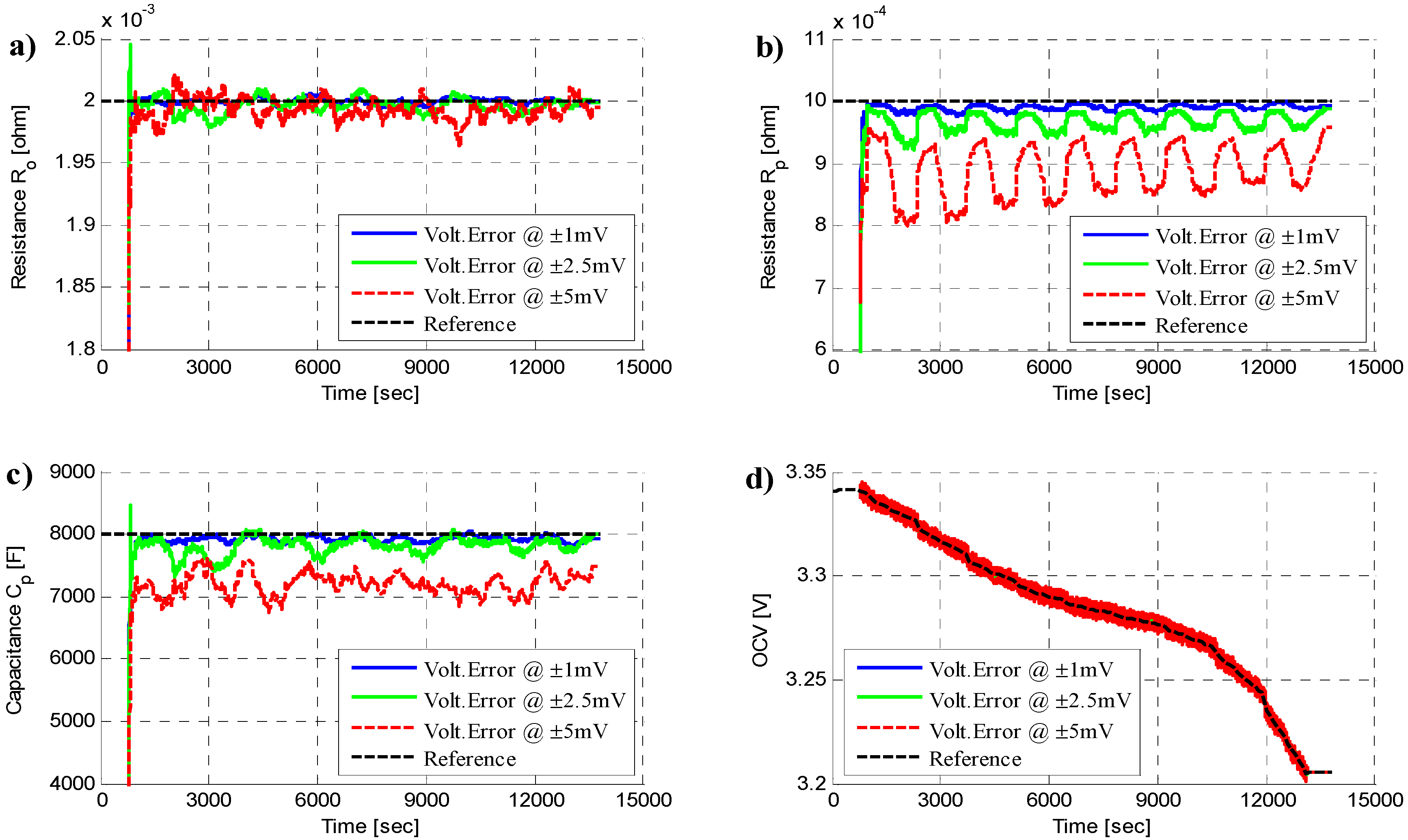
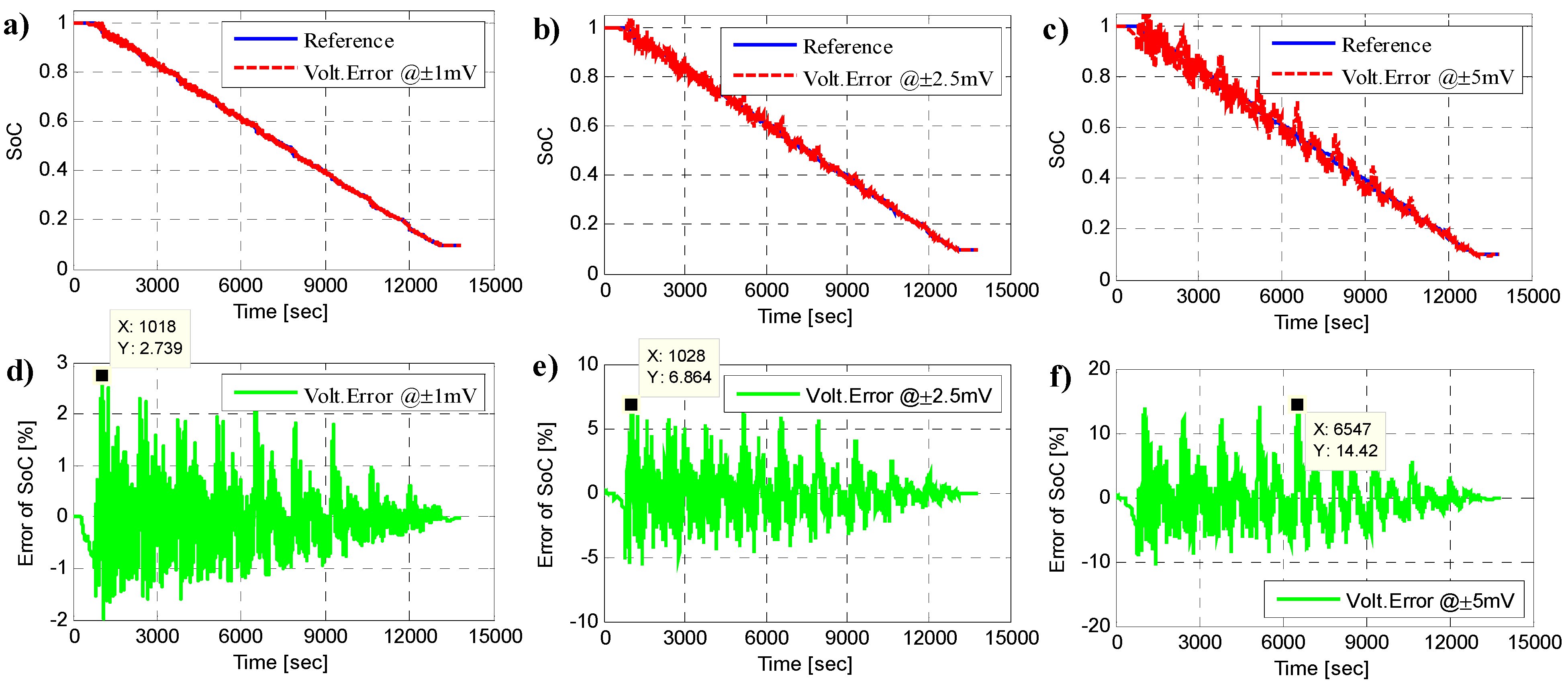
5.3. Voltage Sensor Accuracy Effect

As for the voltage sensor, the accuracy issue will occur with the adaptation of analogue and digital elements, the rounding error of MCU, the sampling alias and harmonics or even electro-magnetic interference, etc. Some typical voltage sensor/transducers with detailed specification [32,33,34] are collected in the following Table 9. From the table, it can be found that the sensor accuracy is varied from ±1.2 mV to ±12.5 mV for different kinds of voltage transducers.

Table 9. The accuracy information comparison of three typical voltage sensors.

Company and product name	Linear Technology Co. LTC6802 (Milpitas, CA, USA)	Texas Instrument Co. bq76PL536 (Dallas, TX, USA)	Maxim Co. MAX11068 (San Jose, CA, USA)
Voltage meas. channels	12	6	12
AD resolution (Bit)	16	14	12
AD conversion time	57 μs	6 μs	10 μs
Typical voltage accuracy	±1.2 mV	±3.0 mV	±12.5 mV
Maximum voltage accuracy	±8.3 mV	±18.0 mV	±50.0 mV
Operating temp. range	−40 °C to +85 °C	−40 °C to +85 °C	−40 °C to +105 °C
Cell balancing	12 channels	6 channels	12 channels
Input voltage range (V)	0–75	0–30	6–72

Table 9. The accuracy information comparison of three typical voltage sensors.

Company and product name	Linear Technology Co. LTC6802 (Milpitas, CA, USA)	Texas Instrument Co. bq76PL536 (Dallas, TX, USA)	Maxim Co. MAX11068 (San Jose, CA, USA)
Voltage meas. channels	12	6	12
AD resolution (Bit)	16	14	12
AD conversion time	57 μs	6 μs	10 μs
Typical voltage accuracy	±1.2 mV	±3.0 mV	±12.5 mV
Maximum voltage accuracy	±8.3 mV	±18.0 mV	±50.0 mV
Operating temp. range	−40 °C to +85 °C	−40 °C to +85 °C	−40 °C to +105 °C
Cell balancing	12 channels	6 channels	12 channels
Input voltage range (V)	0–75	0–30	6–72

To evaluate the effect of voltage precisions on model parameters and SoC estimation, three voltage accuracies of ±1/±2.5/±5 mV are adopted in the simulation. Figure 10 is the estimation results of the model parameters under the FUDS loading profiles. Figure 10a shows the estimated ohmic resistance R_o and its reference value. It indicates that the maximum estimation error of R_o increases from 0.3351% to 1.7986% with the voltage sensor accuracy increased from ±1 mV to ±5 mV. Figure 10b,c lists the estimated polarization resistance R_p and polarization capacitance C_p respectively. When the voltage sensor precision is ±1 mV, the maximum estimation errors of R_p and C_p are 2.5103% and 2.3691%. As the voltage sensor precision rises to ±5 mV, the maximum estimation errors of R_p and C_p ascends abundantly to 20.7418% and 15.9086%. Finally, the estimated OCV is plotted in Figure 10d. It reveals that the maximum estimation error of OCV varies from 0.7227 mV to 3.4698 mV, which is nearly in accordance with voltage precisions. The statistical error analysis of model parameters and SoC, such as maximum error and RMSE is shown in Table 10.

Figure 10. Estimated parameters: (a) R_o, (b) R_p, (c) C_p, and (d) OCV at the voltage sensor precisions of ±1/±2.5/±5 mV.

Figure 10. Estimated parameters: (a) R_o, (b) R_p, (c) C_p, and (d) OCV at the voltage sensor precisions of ±1/±2.5/±5 mV.

Table 10. The statistical error analysis of model parameters and SoC at the voltage sensor precisions of ±1/±2.5/±5 mV.

Item	Voltage accuracy: ±1 mV				Voltage accuracy: ±2.5 mV				Voltage accuracy: ±5 mV
Parameters	Ro	Rp	Cp	SoC	Ro	Rp	Cp	SoC	Ro	Rp	Cp	SoC
Maximum error (%)	0.33	2.51	2.36	2.73	1.08	7.79	8.52	6.86	1.79	20.74	15.9	14.42
RMSE (%)	0.11	1.08	1.07	0.54	0.34	3.64	2.88	1.64	0.51	12.01	10.11	3.54

Table 10. The statistical error analysis of model parameters and SoC at the voltage sensor precisions of ±1/±2.5/±5 mV.

Item	Voltage accuracy: ±1 mV				Voltage accuracy: ±2.5 mV				Voltage accuracy: ±5 mV
Parameters	Ro	Rp	Cp	SoC	Ro	Rp	Cp	SoC	Ro	Rp	Cp	SoC
Maximum error (%)	0.33	2.51	2.36	2.73	1.08	7.79	8.52	6.86	1.79	20.74	15.9	14.42
RMSE (%)	0.11	1.08	1.07	0.54	0.34	3.64	2.88	1.64	0.51	12.01	10.11	3.54

Figure 11 is the estimation results of SoC and SoC errors for three different voltage sensor precisions under the FUDS loading profiles. It shows that the maximum SoC estimation errors for three voltage accuracies are 2.7387%, 6.8638% and 14.4207%. This simulation reveals that there is an effect of current sensor precisions on the SoC estimation accuracy. In the engineering application, to achieve the higher precise estimation for SoC (<5%), the voltage sensor accuracy should be limited to less than ±2 mV.

Figure 11. SoC estimation results at the voltage sensor precisions of (a) ±1 mV, (b) ±2.5 mV, (c) ±5 mV; and the SoC error at the voltage sensor precisions of (d) ±1 mV, (e) ±2.5 mV, (f) ±5 mV.

Figure 11. SoC estimation results at the voltage sensor precisions of (a) ±1 mV, (b) ±2.5 mV, (c) ±5 mV; and the SoC error at the voltage sensor precisions of (d) ±1 mV, (e) ±2.5 mV, (f) ±5 mV.

5.4. Results Comparison and Discussion

Through the comparison of the simulation results, as shown in Figure 12, four meaningful results can be drawn:

(1)

The variation of sampling periods (0.1–1 s) has a significant impact on parameter estimation accuracy. Specifically, the sampling time has a relatively small effect to estimate the ohmic resistance R_o, with the maximum error of 2%. However, the sampling time presents the significant influence for polarization resistance R_p and polarization capacitance C_p with the maximum error of 23%. This result is verification of the previous parameter sensitivity analysis, which means the raised parameter sensitivity of R_p and C_p will be more sensitive to external perturbations. Therefore, an accurate estimate of the R_p and C_p will encounter greater difficulty. On the other hand, the variation of sampling rate has a less significant effect on the SoC estimation error. Therefore, changing the sampling time is not the optimal choice to obtain improved estimation accuracy of the SoC.

(2)

The variation of current sensor precisions (±5/±50/±500 mA) shows little influence for model parameters estimation. For instance, when the current sensor accuracy is ±500 mA, the maximum error of R_p and C_p is about 3.5% and the maximum error of SoC is about 2.76%. Therefore, to restrict the estimation accuracy of the model parameters and SoC, the current sensor accuracy is recommended to be lesser than ±50 mA.

(3)

The variation of voltage sensor precisions (±1/±2.5/±5 mV) has significant impact both on model parameter estimation and on SoC estimation. When the voltage accuracy is ±5 mV, the maximum estimation error of R_o, R_p and C_p is 1.79%, 20.74% and 15.90%, respectively. It reveals that the error of R_o is acceptable, while the error of R_p and C_p is hardly acceptable. As the voltage accuracy decreases to ±1 mV, the maximum estimation error of R_o, R_p and C_p is in the acceptable range of 0.33%, 2.51% and 2.36%. For the SoC estimation, the maximum SoC error increases from 2.73%, 6.86% to 14.42%, as the voltage sensor accuracy ascends from ±1 mV, ±2.5 mV to ±5 mV. Therefore, to ensure an accurate SoC estimation (<5%), the voltage sensor precision should be less than ±2 mV. This conclusion can also be drawn from the ICA result.

(4)

The weighted importance of factors on parameters and SoC estimation can be sorted as (by descending order): voltage sensor accuracy > sampling period > current sensor accuracy based on the above comparison.

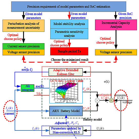
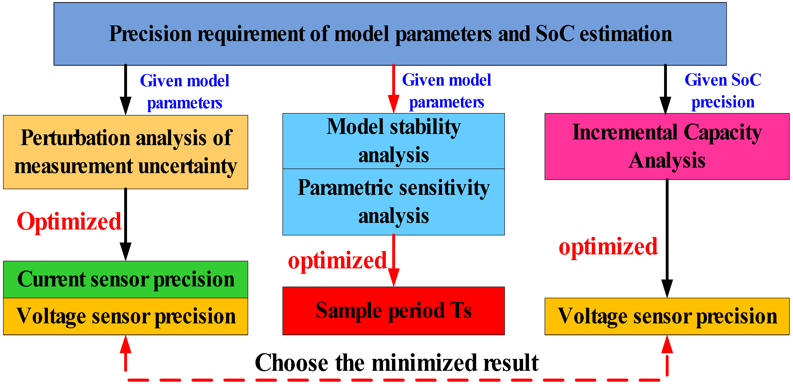
Figure 12. Comparison of three factors on the stability of model parameters and SoC estimation: (a) R_o, (b) R_p, (c) C_p, and (d) SoC.

Figure 12. Comparison of three factors on the stability of model parameters and SoC estimation: (a) R_o, (b) R_p, (c) C_p, and (d) SoC.

In general, the optimal selection approach for time sampling period T_s, current/voltage sensor precisions, as shown in Figure 13, could be summarized as:

(a)

Firstly assess the parameters of battery system, such as R_o, R_p, C_p and capacity, then conduct the perturbation analysis with the Equations (9)–(11) according to the precision requirement of model parameters. The optimized current/voltage sensor precision could be computed.

(b)

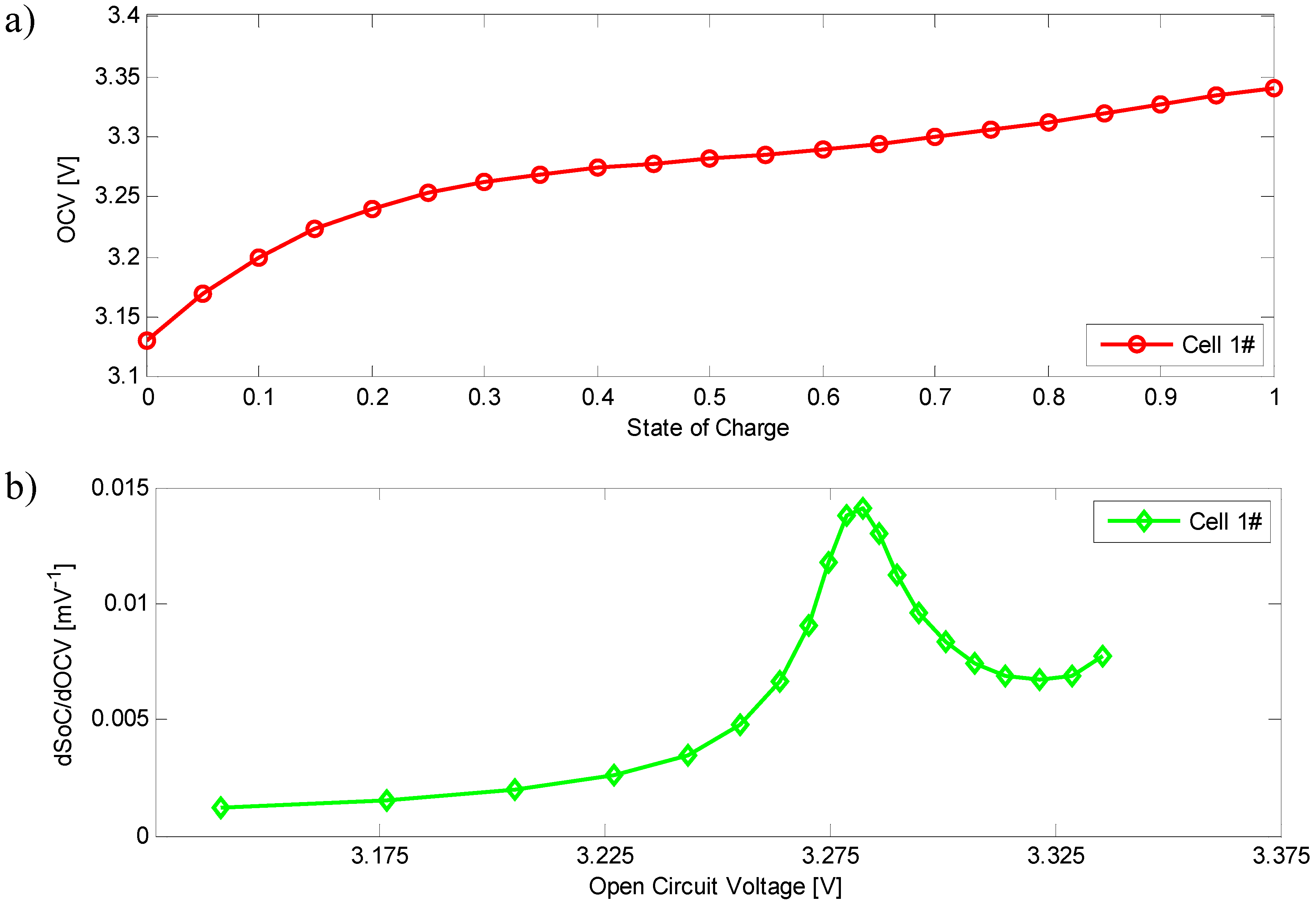
About the given SoC precision requirement, the user can calculate the voltage precision with the ICA. Take this research for example: If the minimal SoC estimation precision is limited as 1.5%, our voltage sensor precision could be calculated as 1.034 mV with the ICA result in Figure 5.

(c)

Compare the voltage precision in Steps (a) and (b), then choose the minimized result. If the minimized result is from Step (a), re-compute Step (a) again to update the current sensor precision.

(d)

About the given model parameters, the user can conduct the model stability analysis and parametric sensitivity analysis. Then the threshold of time sampling period T_s could be gain. The optimized time sampling period T_s could be selected in a tradeoff way by considering the model stability, parametric sensitivity, system-sampling precision and the hardware runtime.

Figure 13. The selection approach for sample period T_s, current/voltage sensor precisions.

Figure 13. The selection approach for sample period T_s, current/voltage sensor precisions.

6. Conclusions

In this paper, the stability of model parameters and SoC estimation have been analyzed and simulated with FUDS profiles. In summary, the main concluding remarks are given as follows:

(1)

The model stability and parametric sensitivity have been analyzed under different sampling periods T_s (0.02, 0.1, 0.2, 0.5 and 1 s). The results reveal that the increase of sampling period T_s will be beneficial to the model stability and parameter identifiability. From an engineering viewpoint, it is recommended to restrict the eigenvalues of the ARX model within a range of 0–0.95. That is, T_s should be larger than one threshold, such as T_s ≥ 0.5 s.

(2)

The variation of sampling periods (0.1–1 s), has a significant impact on parameter estimation accuracy but a less significant effect on the SoC estimation error. Therefore, to improve the estimation accuracy of the SoC, it is not optimal to change the sampling time.

(3)

The variation of current sensor precision (±5/±50/±500 mA) shows little influence for model parameters and SoC estimation. To restrict the estimation accuracy of the model parameters and SoC, the current sensor accuracy is recommended to be less than ±50 mA.

(4)

The variation of voltage sensor precision (±1/±2.5/±5 mV) has significant impact on both the model parameter estimation and SoC estimation. To ensure the SoC estimation accuracy (<5%), the voltage sensor accuracy should be less than ±2 mV.

(5)

According to the parameter variation analysis under the perturbation of current/voltage measurement uncertainty, the weighted importance of factors on parameter and SoC estimation can be sorted as (by descending order): voltage sensor accuracy > sampling period > current sensor accuracy.

References

1. He, H.; Xiong, R.; Zhang, X.; Sun, F.; Fan, J. State-of-charge estimation of the lithium-ion battery using an adaptive extended Kalman filter based on an improved thevenin model. IEEE Trans. Veh. Technol. 2011, 60, 1461–1469. [Google Scholar]
2. He, Z.; Gao, M.; Wang, C.; Wang, L.; Liu, Y. Adaptive state of charge estimation for Li-ion batteries based on an unscented Kalman filter with an enhanced battery model. Energies 2013, 6, 4134–4151. [Google Scholar] [CrossRef]
3. Xing, Y.; He, W.; Pecht, M.; Tsui, K.L. State of charge estimation of lithium-ion batteries using the open-circuit voltage at various ambient temperatures. Appl. Energy 2014, 113, 106–115. [Google Scholar] [CrossRef]
4. Wang, Y.; Zhang, C.; Chen, Z. A method for joint estimation of state-of-charge and available energy of LiFePO4 batteries. Appl. Energy 2014, 135, 81–87. [Google Scholar] [CrossRef]
5. Liu, X.; Wu, J.; Zhang, C.; Chen, Z. A method for state of energy estimation of lithium-ion batteries at dynamic currents and temperatures. J. Power Sources 2014, 270, 151–157. [Google Scholar] [CrossRef]
6. Xiong, R.; Sun, F.; Chen, Z.; He, H. A data-driven multi-scale extended Kalman filtering based parameter and state estimation approach of lithium-ion olymer battery in electric vehicles. Appl. Energy 2014, 113, 463–476. [Google Scholar] [CrossRef]
7. Xiong, R.; Sun, F.; Gong, X.; Gao, C. A data-driven based adaptive state of charge estimator of lithium-ion polymer battery used in electric vehicles. Appl. Energy 2014, 113, 1421–1433. [Google Scholar] [CrossRef]
8. Dai, H.; Wei, X.; Sun, Z.; Wang, J.; Gu, W. Online cell SOC estimation of Li-ion battery packs using a dual time-scale Kalman filtering for EV applications. Appl. Energy 2012, 95, 227–237. [Google Scholar] [CrossRef]
9. Zhong, L.; Zhang, C.; He, Y.; Chen, Z. A method for the estimation of the battery pack state of charge based on in-pack cells uniformity analysis. Appl. Energy 2014, 113, 558–564. [Google Scholar] [CrossRef]
10. Liu, X.; Chen, Z.; Zhang, C.; Wu, J. A novel temperature-compensated model for power Li-ion batteries with dual-particle-filter state of charge estimation. Appl. Energy 2014, 123, 263–272. [Google Scholar] [CrossRef]
11. Hu, X.; Li, S.; Peng, H.; Sun, F. Charging time and loss optimization for linmc and LiFePO4 batteries based on equivalent circuit models. J. Power Sources 2013, 239, 449–457. [Google Scholar] [CrossRef]
12. Xiong, R.; Gong, X.; Mi, C.C.; Sun, F. A robust state-of-charge estimator for multiple types of lithium-ion batteries using adaptive extended Kalman filter. J. Power Sources 2013, 243, 805–816. [Google Scholar] [CrossRef]
13. Plett, G.L. Extended Kalman filtering for battery management systems of LiPB-based HEV battery packs: Part 1. Background. J. Power Sources 2004, 134, 252–261. [Google Scholar] [CrossRef]
14. Plett, G.L. Extended Kalman filtering for battery management systems of LiPB-based HEV battery packs: Part 2. Modeling and identification. J. Power Sources 2004, 134, 262–276. [Google Scholar] [CrossRef]
15. Plett, G.L. Extended Kalman filtering for battery management systems of LiPB-based HEV battery packs: Part 3. State and parameter estimation. J. Power Sources 2004, 134, 277–292. [Google Scholar] [CrossRef]
16. Yuan, S.; Wu, H.; Yin, C. State of charge estimation using the extended Kalman filter for battery management systems based on the arx battery model. Energies 2013, 6, 444–470. [Google Scholar] [CrossRef]
17. Han, J.; Kim, D.; Sunwoo, M. State-of-charge estimation of lead-acid batteries using an adaptive extended Kalman filter. J. Power Sources 2009, 188, 606–612. [Google Scholar] [CrossRef]
18. Sun, F.; Hu, X.; Zou, Y.; Li, S. Adaptive unscented Kalman filtering for state of charge estimation of a lithium-ion battery for electric vehicles. Energy 2011, 36, 3531–3540. [Google Scholar] [CrossRef]
19. Santhanagopalan, S.; White, R.E. State of charge estimation using an unscented filter for high power lithium ion cells. Int. J. Energy Res. 2010, 34, 152–163. [Google Scholar] [CrossRef]
20. Shao, S.; Bi, J.; Yang, F.; Guan, W. On-line estimation of state-of-charge of Li-ion batteries in electric vehicle using the resampling particle filter. Transp. Res. Part D 2014, 32, 207–217. [Google Scholar] [CrossRef]
21. Gao, M.; Liu, Y.; He, Z. Battery State of Charge Online Estimation Based on Particle Filter. In Preoceeeings of the 2011 4th International Congress on Image and Signal Processing (CISP), Shanghai, China, 15–17 October 2011; IEEE: New York, NY, USA, 2011; pp. 2233–2236. [Google Scholar]
22. Hu, X.; Sun, F.; Zou, Y. Estimation of state of charge of a lithium-ion battery pack for electric vehicles using an adaptive luenberger observer. Energies 2010, 3, 1586–1603. [Google Scholar] [CrossRef]
23. Kim, I.-S. The novel state of charge estimation method for lithium battery using sliding mode observer. J. Power Sources 2006, 163, 584–590. [Google Scholar] [CrossRef]
24. Xia, B.; Chen, C.; Tian, Y.; Sun, W.; Xu, Z.; Zheng, W. A novel method for state of charge estimation of lithium-ion batteries using a nonlinear observer. J. Power Sources 2014, 270, 359–366. [Google Scholar] [CrossRef]
25. Zhang, X.; Mi, C. Vehicle Power Management: Modeling, Control and Optimization; Springer: Berlin/Heidelberg, Germany, 2011. [Google Scholar]
26. Hu, X.; Sun, F.; Zou, Y.; Peng, H. Online Estimation of an Electric Vehicle Lithium-Ion Battery Using Recursive Least Squares with Forgetting. In Preoceeeings of the American Control Conference (ACC), San Francisco, CA, USA, 29 June–1 July 2011; IEEE: New York, NY, USA, 2011; pp. 935–940. [Google Scholar]
27. Feng, D.; Tongwen, C.; Li, Q. Bias compensation based recursive least-squares identification algorithm for MISO systems. IEEE Trans. Circuits Syst. II Express Briefs 2006, 53, 349–353. [Google Scholar] [CrossRef]
28. Wu, H.; Yuan, S.; Zhang, X.; Yin, C.; Ma, X. Model parameter estimation approach based on incremental analysis for lithium-ion batteries without using open circuit voltage. J. Power Sources 2015, 287, 108–118. [Google Scholar] [CrossRef]
29. Xiong, R.; He, H.; Sun, F.; Liu, X.; Liu, Z. Model-based state of charge and peak power capability joint estimation of lithium-ion battery in plug-in hybrid electric vehicles. J. Power Sources 2013, 229, 159–169. [Google Scholar] [CrossRef]
30. Lem—Current Tranducer, Voltage Transducer, Sensor, Power Measurement. Available online: http://www.lem.com/ (accessed on 26 June 2015).
31. Allegro MicroSystems LLC. Available online: http://www.allegromicro.com/ (accessed on 26 June 2015).
32. Linear Technology—Home Page. Available online: http://www.linear.com/index.php (accessed on 26 June 2015).
33. Analog, Embedded Processing, Semiconductor Company, Texas Instruments—TI.Com. Available online: http://www.ti.com/ (accessed on 26 June 2015).
34. Maxim Integrated. Analog, Linear, and Mixed-Signal Devices from Maxim. Available online: http://www.maximintegrated.com/en.html (accessed on 26 June 2015).