4.1. Deterministic Wind Power Forecasts
Figure 2 shows the
MAE trends for the Abruzzo test case, whose evaluation is carried out on 0–72 h ahead forecast lead times with 3-h time-steps.
MAE values are also calculated on the whole forecast range for the ranking, and are reported in
Figure 2.
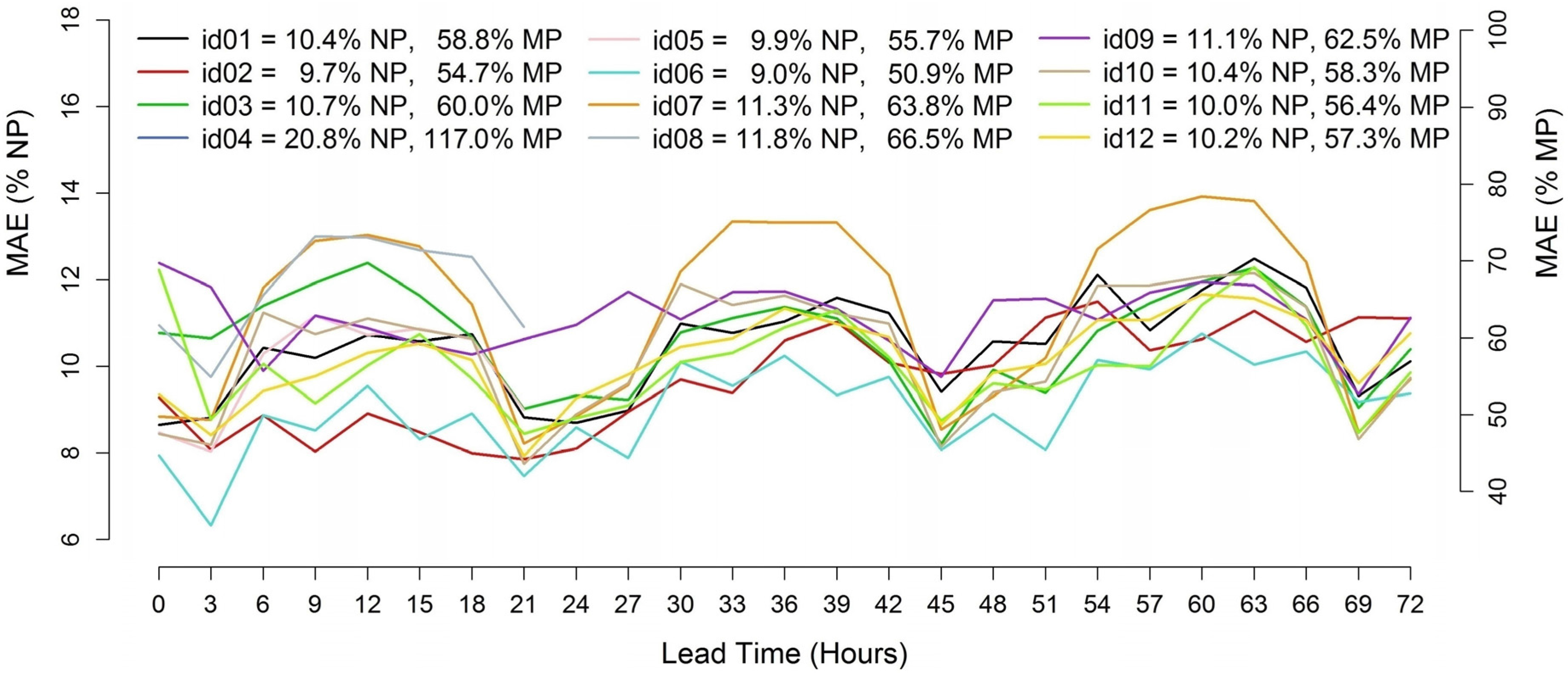
Figure 2.
Error trends of the 0–72 h ahead wind power forecasts starting at 12 UTC for the Abruzzo test case (MAE/NP % and MAE/MP %). MAE: mean absolute error; NP: nominal power; and MP: mean power.
Figure 2.
Error trends of the 0–72 h ahead wind power forecasts starting at 12 UTC for the Abruzzo test case (MAE/NP % and MAE/MP %). MAE: mean absolute error; NP: nominal power; and MP: mean power.
Except for a clear outlier, similar MAE trends are observed, with slightly higher errors for larger lead times. There is, however, a significant difference between the lowest and the highest MAE, which span in about 4 or 5 MAE/NP percentage points, depending on the lead time. Almost all the models show a strong daily cycle with larger MAE values during evening and night hours. Looking at the MAE/MP values, it can be noticed that most of the forecasts range between 50% and 65%, depending on the forecast horizon. The best result is achieved by id06 with a total MAE/NP of 9.0% and a MAE/MP of 50.9%. The DM test applied comparing id06 to the second best (id02, 9.7% MAE/NP and 54.7% MAE/MP) returns a p-value of 3.91 × 10⁻⁶, allowing rejection of the hypothesis that the forecasts have the same accuracy.
The results for the Klim wind farm are shown in
Figure 3. In this case, 0–48 h ahead, hourly forecasts are evaluated, considering all four initialization times (
i.e., 00, 06, 12 and 18 UTC) together.
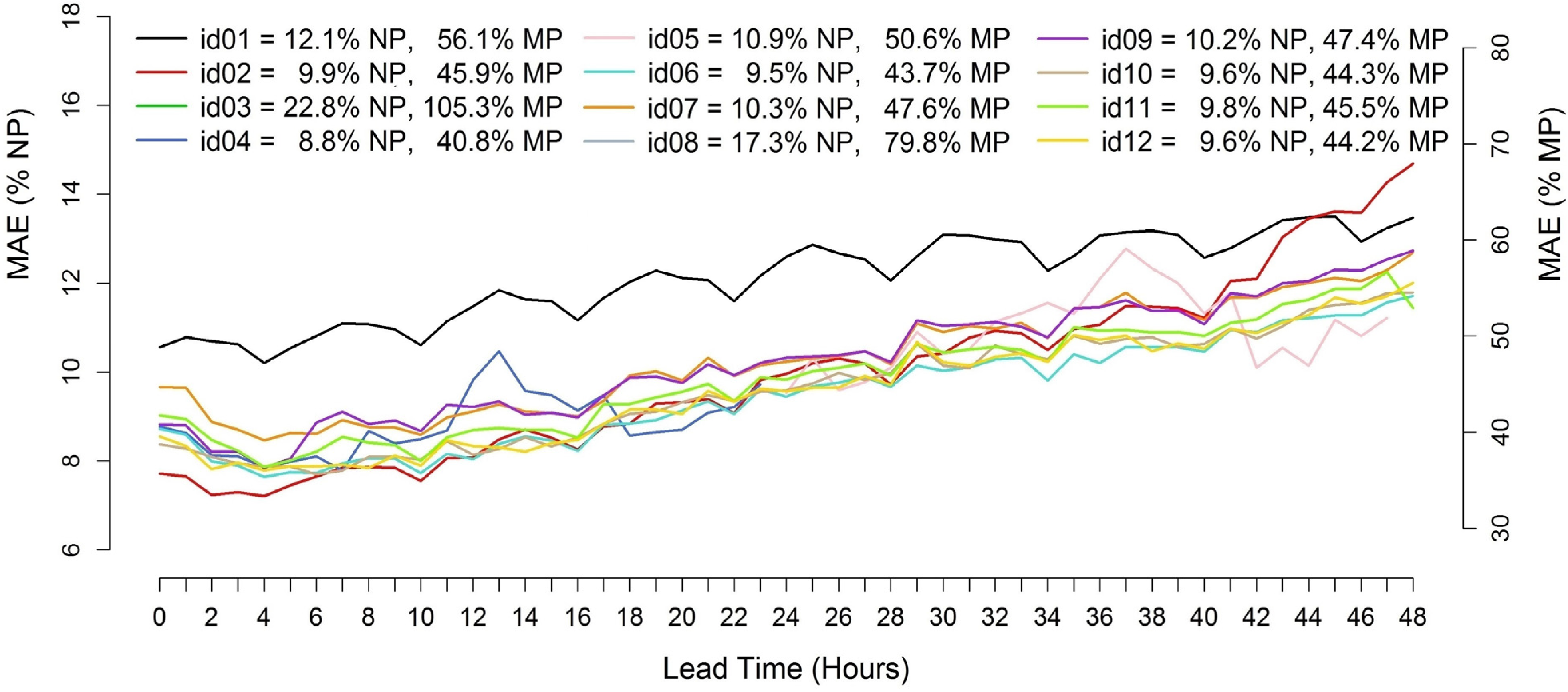
The results show a best score of 9.5% MAE/NP and 43.7% MAE/MP, achieved again by id06. The outcome of 8.8% MAE/NP achieved by id04 is not considered, since the participant just provided forecasts for the 0–23 h ahead horizon without considering longer lead times. It is possible to observe a more defined trend with increasing MAE values for larger lead times than for Abruzzo, but with considerably lower dispersion of the error values (i.e., about 1–2 MAE/NP percentage points, depending on the lead time). There are also a couple of outliers probably caused by some basic mistakes in the forecasting method. The DM test applied to id06 versus the second best (i.e., id12, 9.6% MAE/NP and 44.2% MAE/MP) returns a p-value of 1.27 × 10–141, meaning that even in this case the hypothesis of same forecast accuracy can be rejected. Overall, some considerations can be drawn with respect to the differences in the error trends between the two sites.
Figure 3.
Error trends of the 0–48 h ahead wind power forecasts starting at 0, 6, 12 and 18 UTC for the Klim test case (MAE/NP % and MAE/MP %).
Figure 3.
Error trends of the 0–48 h ahead wind power forecasts starting at 0, 6, 12 and 18 UTC for the Klim test case (MAE/NP % and MAE/MP %).
Abruzzo is characterized by a strong daily cycle of power production, which is not observed at Klim. Higher errors during night at Abruzzo are due to higher production during those hours, in fact the average wind power at 0 UTC is 6% higher than at 12 UTC. The authors believe that the increasing trend over lead time observed at Klim is related to the kind of error characterizing the meteorological forecasts. In fact, Klim is located on a flat terrain, where the meteorological forecasts are affected by lower representativeness errors (bad representations of topography, land use, kinematic winds
etc.), which are higher for complex-terrain sites like Abruzzo. These kinds of error mask those caused by the decreasing predictability of the atmospheric flows over lead time more at Abruzzo than at Klim.
Table 4 reports model bias with respect to
NP for both Abruzzo and Klim. Bias is computed as average over the whole forecast period.
Table 4.
Model bias for Abruzzo and Klim. Bias is expressed as percentage of NP.
Table 4.
Model bias for Abruzzo and Klim. Bias is expressed as percentage of NP.
| Power plant | id01 | id02 | id03 | id04 | id05 | id06 | id07 | id08 | id09 | id10 | id11 | id12 |
|---|
| Abruzzo | 1.6 | 0.9 | 2.4 | 2.1 | 1.1 | 0.7 | 5.3 | 0.9 | 0.4 | 0.7 | 0.5 | 4.4 |
| Klim | −2.9 | −0.5 | 0.0 | 3.2 | 0.0 | −0.5 | −2.5 | 2.3 | −2.4 | 0.3 | −1.5 | 1.9 |
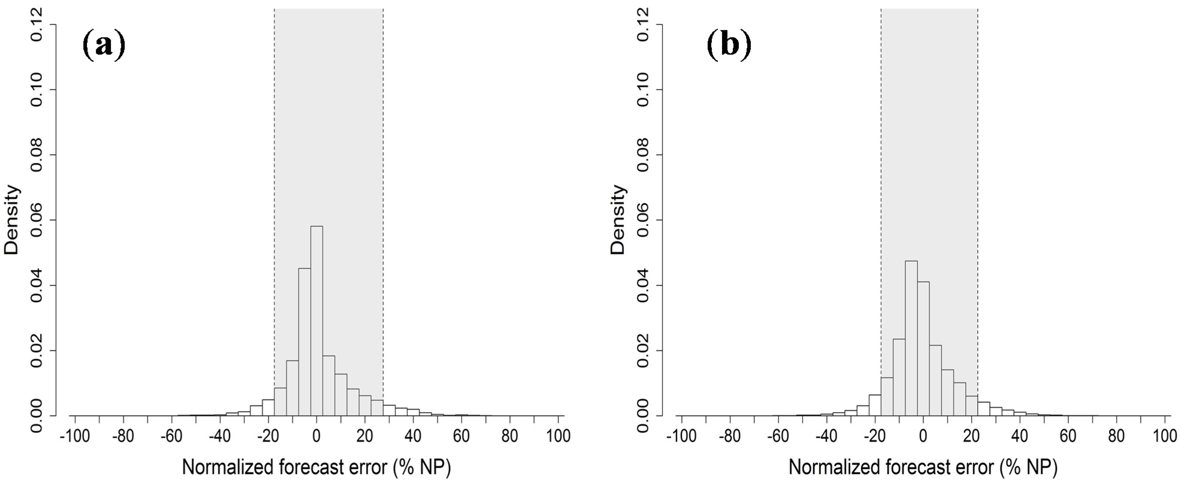
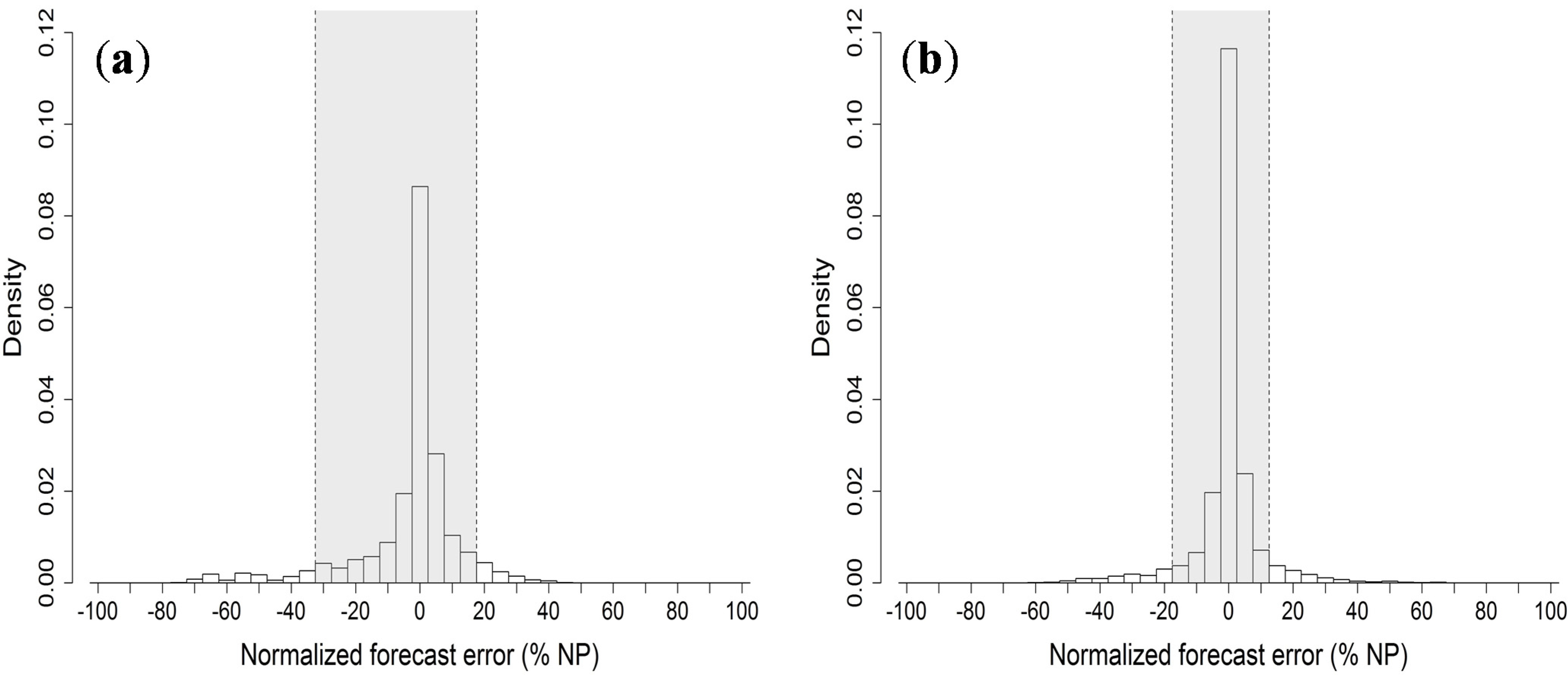
It is possible to extract more information from the error distributions calculated from the best forecast of each test case. The diagrams, produced for the whole forecast range with bins representing 5% of
NP, are reported in
Figure 4.
The grey shaded area in each histogram delimits the 5%–95% quantiles interval. In both cases, a tendency to slightly overestimate wind power is noticeable from the positive skew in lower bins, especially for the Klim case. The distribution obtained for Abruzzo is slightly sharper than the one for Klim and shows prediction errors lower than 7.5% of NP 67% of the times, while for Klim this happens in 62% of the cases.
Figure 4.
Error distributions (id06) of the best forecasts for the Abruzzo case (a) and the Klim case (b). The grey area in each histogram delimits the 5%–95% quantiles interval.
Figure 4.
Error distributions (id06) of the best forecasts for the Abruzzo case (a) and the Klim case (b). The grey area in each histogram delimits the 5%–95% quantiles interval.
In both test cases id06 achieves the best result. His forecasting method is based on the use of meteorological data provided by COST and an application of two statistical approaches combining artificial neural networks (ANN) and generalized linear models (GLM) [
28]. The two methods were used separately to learn the non-linear relation between the historical weather forecasts and the wind farm power measurements. The ANN consists in a feed-forward multilayer perceptron with one hidden layer and was optimized with the Levenberg-Marquardt algorithm. In the GLM, a logit function was applied as a link function and the response variable (
i.e., wind power) was assumed to be binomially distributed. Wind power production data was normalized between 0 and 1 by division with
NP. The forecasts of all meteorological parameters were standardized and used as model input together with information about the time of day. ANN and GLM used the same set of input data. Before training the models, power data was filtered manually with respect to non-plausible values. The outputs of the ANN and GLM were then averaged to get a final wind power forecast for each wind farm.
Concerning the forecasting methods used by other participants, it should be noticed that most of them consist of different post-processing techniques applied to the NWP data provided by the organizers.
ANNs were used (e.g., id02, id05) with variable performance depending on the case. In the case of id10, forecasting the average of an ensemble of ANN initialized with different weights proves to be quite effective, ranking third on the Klim case. A method based on a combination of time series and approximation (id11) also led to good performance on both power plants.
Further methods were based on other machine-learning techniques, e.g., support vector machines (SVM): id04 applied SVM with fairly good results on Klim, providing forecasts only for the 0–24 h ahead interval; id01 chose to run a non-hydrostatic multi-nested model followed by a combination of Kalman Filter, ANN and Ensemble Learning techniques as post-processing, but with less effective results especially in the case of Klim; id07 used a fitting methodology that divided sample data into bins and computed a power series by minimizing the variance between power values inside the bins and the fitting power, obtaining a power curve by linear interpolation between the fitting power values. The approach was, however, not so effective, especially on Abruzzo.
A Computational Fluid Dynamics (CFD) model was applied by id08, but the lack of data regarding the wind farms (i.e., single turbine data, anemometer measurements on site) didn’t allow setting up a complete post-process and thus obtaining good results.
For Abruzzo, the second best result is obtained by id02 using additional meteorological data from the GFS global model, followed by application of a wind farm model (accounting for wake parameterization based on atmospheric stability) and reconstruction of a density corrected power curve. Data were also processed by an ANN. For Klim, the second best result is achieved by id12 with a hybrid approach combining physical modeling and advanced statistical post-processing, including a combination model applied on different prediction feeds.
4.2. Klim Case—Comparison with Previous Benchmark and High Resolution Model Run
As previously explained, forecast data for Klim are the same used back in 2002 and tested in [
18]. HIRLAM spatial resolution at that time was equal to 0.15°, and it was driven by the ECMWF boundary conditions fields with 0.5° resolution. In
Figure 5, a comparison between the new results obtained during the current exercise and the results obtained in [
18] is addressed. It should be noticed that the amount of available data in [
18] was higher. In particular, 2 years of data were used as a training period (from January 1999 to February 2001), while forecast evaluation was performed on data from March 2001 to April 2003.
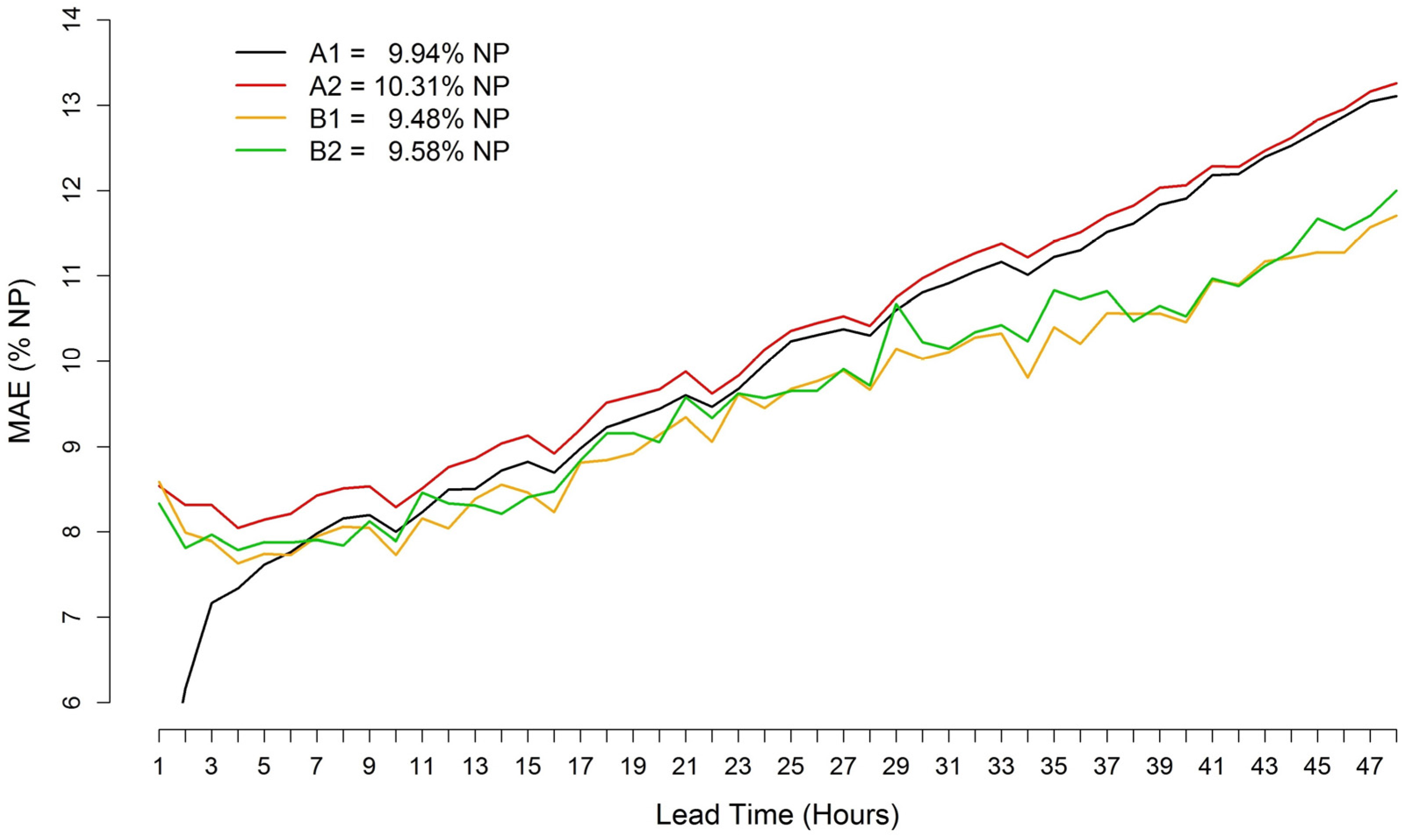
Figure 5 compares the
MAE as a function of forecast lead time of the best two forecasts from the previous benchmark and the current exercise. In this comparison data for lead time 0 is missing, in fact it wasn’t evaluated at that time. As in
Figure 3, the forecasts are compared considering all four initialization times together.
Figure 5.
Comparison between new and old results in term of MAE/NP as a function of forecast lead time (1–48 h ahead) for the wind power forecasts issued at 0, 6, 12 and 18 UTC for the Klim test case. A1, A2 and B1, B2 are the best 2 forecasts of the previous benchmark and the current work respectively.
In the diagram, A1 and A2 are the best 2 forecasts issued for [
18], while B1 and B2 correspond to the best forecasts of the current exercise. B1 and B2 are generally better in terms of
MAE, especially for the forecast horizon from 24 h to 48 h ahead. During the previous benchmark some participants used models with auto-adaptive capabilities, which can benefit e.g., from using available online data. This appears evident looking at the A1 case, outperforming the others up to 5 h ahead. For longer lead times, however, the performance of A1 degrades and remains lower than those of B1 and B2. This is likely due to an improvement in the statistical post-processing techniques adopted by B1 and B2.
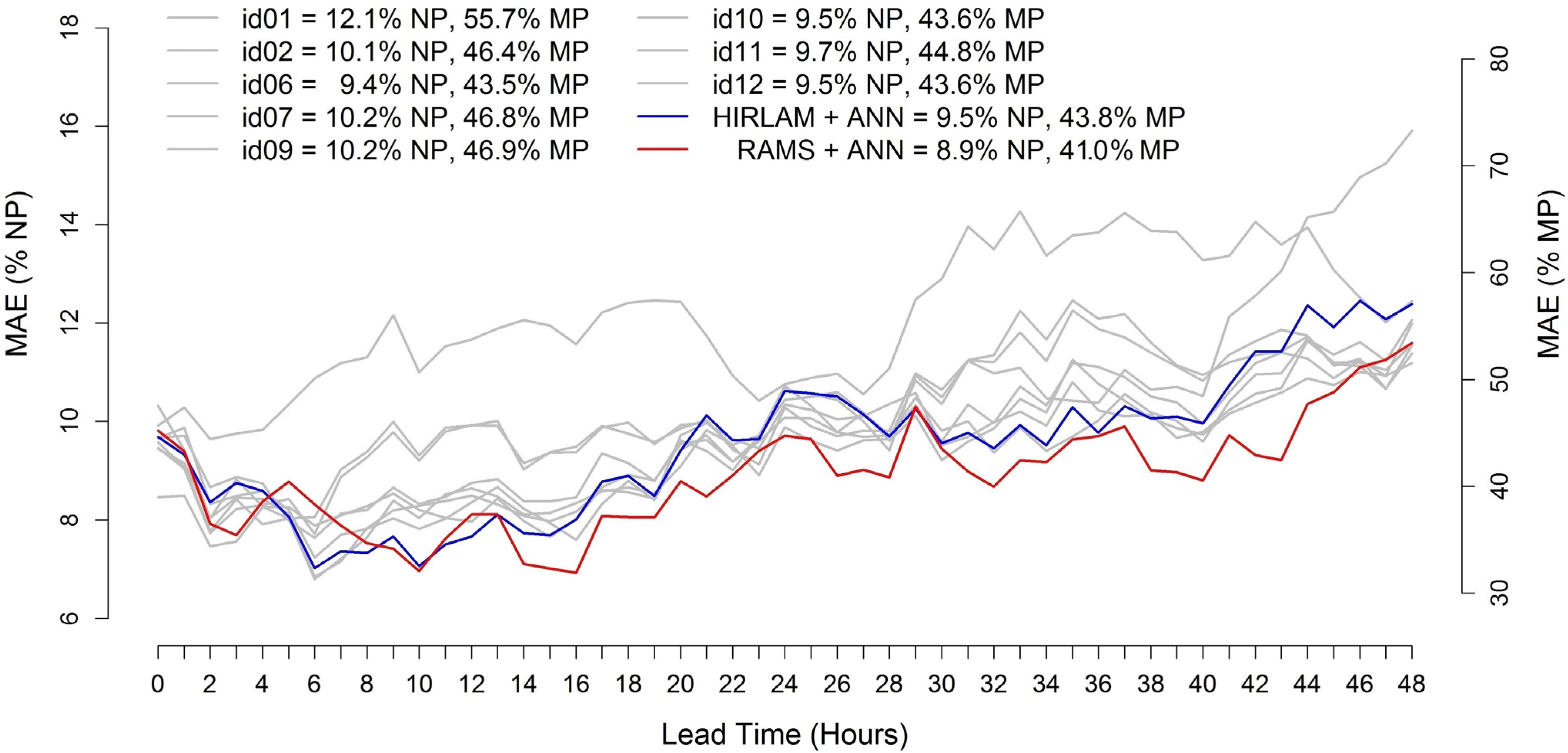
Furthermore, in order to investigate the potential improvement achievable by using higher resolution forecasts for the same power plant, the organizers have performed a new forecast run using RAMS. These forecasts were not provided for the exercise: however, a comparison with its results is addressed here.
ECMWF reforecast data with 0.25° horizontal resolution were retrieved for the same 2-year period. RAMS runs starting at 12 UTC using 2 nested grids with horizontal resolution of 12 km and 4 km were performed. Therefore, higher resolutions in both boundary conditions and the limited-area model were used. A post-processing system based on an ANN [
29,
30] was applied to both RAMS and HIRLAM output. As a consequence, the post-processing model is similar to the one used by the winner in the exercise, even if the GLM part was not performed. For this test the same conditions imposed on the participants were maintained (
i.e., missing data for the first 14 days of each month of the test period).
Figure 6 shows the
MAE/
NP and
MAE/
MP as a function of forecast lead time, calculated only for the 12 UTC model runs. The results obtained by all participants are shown in grey while the red line refers to the model chain RAMS + ANN. Results obtained by the ANN post-processing applied to HIRLAM data (HIRLAM + ANN) are also reported in blue.
Figure 6.
Error trends of the 0–48 h ahead wind power forecasts starting at 12 UTC for the Klim test case (MAE/NP % and MAE/MP %).
Figure 6.
Error trends of the 0–48 h ahead wind power forecasts starting at 12 UTC for the Klim test case (MAE/NP % and MAE/MP %).
With 8.9% MAE/NP and 41.0% MAE/MP, RAMS + ANN allowed gaining about 0.5% of MAE/NP and 2.5% of MAE/MP on the best result observed during the exercise. The application of HIRLAM + ANN allowed obtaining similar results as those obtained by other participants, with 9.5% MAE/NP and 43.8% MAE/MP. The application of the DM test on RAMS+ANN versus the result obtained by id06 returns a p-value of 9.2 × 10⁻², which allows rejecting the null hypothesis (i.e., RAMS+ANN results to be better than id06).
The improvement shown by RAMS+ANN provides evidence of the benefits of using a higher spatial resolution both in the boundary conditions (which have been improved in the last 10 years due to the development carried out on the ECMWF deterministic model) and also in the limited area model. However, other model improvements like data assimilation schemes and physics parameterizations can also have contributed to increase the performance.
4.3. Deterministic Solar Power Forecasts
Solar statistics are computed on forecast data filtered using solar height (
i.e., forecasts in correspondence of lead times with solar height equal to zero are discarded).
Figure 7 displays the
MAE trends for Milano, calculated for the 3–72 h ahead forecast interval with 3-hourly time-steps. Two outliers behave very differently from the other models, especially during the 3–6 h ahead interval. Apart from these, a common trend between the different models is observed with the forecast errors reaching their peaks at 12 UTC of each forecast day. The difference between the error values of different models ranges between 2% and 3% of
MAE/
NP. The best score is obtained by id07 with an
MAE/
NP of 7.0% and an
MAE/
MP of 30.1%. The DM test applied comparing id07 with id01 (7.4%
MAE/
NP and 31.7%
MAE/MP) returns a
p-value of 0.961. It is thus difficult to state whether one model is actually more accurate than the other, and the null hypothesis cannot be rejected.
Figure 7.
Error trends of the 3–72 h ahead solar power forecasts starting at 12 UTC for the Milano test case (MAE/NP % and MAE/MP %).
Figure 7.
Error trends of the 3–72 h ahead solar power forecasts starting at 12 UTC for the Milano test case (MAE/NP % and MAE/MP %).
Figure 8 shows the
MAE trend for the 1–72 h ahead, hourly forecasts made for Catania with hourly time-steps.
Figure 8.
Error trends of the 1–72 h ahead solar power forecasts starting at 0 UTC for the Catania test case (MAE/NP % and MAE/MP %).
Figure 8.
Error trends of the 1–72 h ahead solar power forecasts starting at 0 UTC for the Catania test case (MAE/NP % and MAE/MP %).
Except for a couple of models which exhibit two peaks during early morning and late afternoon hours, all the others show a maximum MAE around 12 UTC. The differences between the models are higher than for Milano test, reaching about 5%. id07 performed again better than the others with a 5.4% MAE/NP and 14.8% MAE/MP. The result is particularly good, with almost 1% MAE/NP less than the second best result of 6.3%, achieved by id09. However, the p-value of 0.999 returned from the DM test prevents rejecting the null hypothesis.
Looking at
Figure 7 and
Figure 8 one could notice that solar power forecasting error trends are strongly dependent on the daily cycle. This is due to the solar elevation trend that partly masks lead time dependent errors. Also, the meteorological model’s skill in forecasting solar irradiance and cloud coverage is not strongly dependent on lead time, and this is reflected on the power predictions. Bias values for both Milano and Catania are reported in
Table 5.
Table 5.
Model bias for Milano and Catania. Bias is expressed as percentage of NP.
Table 5.
Model bias for Milano and Catania. Bias is expressed as percentage of NP.
| Power plant | id01 | id02 | id03 | id04 | id05 | id06 | id07 | id08 | id09 |
|---|
| Milano | −1.3 | 0.2 | 3.3 | −10.6 | 0.9 | −0.7 | 0.0 | −2.2 | - |
| Catania | 1.5 | 3.8 | 0.6 | −1.5 | −1.7 | 8.7 | −0.4 | 1.0 | 0.8 |
Error distributions obtained by id07 are investigated using the diagrams shown in
Figure 9. Comparing the two histograms with those calculated on wind power, sharper and narrower distributions for both the Milano and Catania tests are seen, which implies a higher level of predictability of solar power in this exercise. Catania, in particular, shows a pretty symmetric distribution, with forecast errors being lower than 7.5% of
NP 83% of the time. The distribution obtained for Milano is less symmetric and shows a higher number of negative errors. For Milano, errors lower than 7.5% are observed in 72% of the cases.
Figure 9.
Error distributions (id07) of the best forecasts for the Milano case (a) and the Catania case (b). The grey area in each histogram delimits the 5%–95% quantiles interval.
Figure 9.
Error distributions (id07) of the best forecasts for the Milano case (a) and the Catania case (b). The grey area in each histogram delimits the 5%–95% quantiles interval.
Similarly to the wind part of the benchmark, one participant achieves the best result in both test cases in the solar application. For Milano, id07 used meteorological data provided by COST as input, then applying a quantile regression in order to estimate a clear sky production, a clear sky irradiance and a medium temperature [
31]. A linear regression was also applied to explain the rate of observed clear sky production. The same method was used for Catania, with the additional step of performing a bias correction with a quantile regression, based on lead time and forecasted power. This last step was not applied to the Milano case due to the reduced amount of available data.
The other methods applied were mainly based on meteorological data provided by the organizers. A method proposed by id01 ranked third on Catania and second on Milano, using non-linear regression techniques such as random forests.
For Catania, the participant with the second best result (
i.e., id09) combined the output of the RAMS model provided by COST with the WRF ARW [
32] model, initialized with boundary conditions from GFS. The forecasting system was (multiple) linear regression with several explanatory variables whose coefficients are estimated from data. Different variables derived from the NWP outputs were used in the regression, and they were fitted simultaneously in one consistent model. The derived variables were: direct component of the solar radiation on the tilted panel (30°, south) from WRF, diffuse component of the solar radiation on the tilted panel from WRF, difference between direct radiation on the tilted panel obtained from WRF and RAMS, difference between di use radiation on the tilted panel obtained from WRF and RAMS, interaction between direct WRF radiation and cosine of the zenith angle and interaction between diffuse WRF radiation and cosine of the zenith angle.
Other participants also applied linear regression techniques: id05 used all available values from GHI and solar power, applying linear regression to derive the relevant coefficients, but the results appear less effective; id08 forecasted the power output with a regression model based on the adjusted solar irradiance incident on the PV model surface and the solar cell temperature, which were calculated with the isotropic sky model and the standard formula with nominal operating cell temperature (NOCT) respectively, obtaining average results on both plants.
Few participants applied machine-learning techniques. ANN with a back-propagation algorithm was used by id06 with average results on Milano.
It should be noted that an SVM based application performed by id04 ranked third on Catania considering only the first prediction day. However, forecasts for the 24–48 h and 48–72 h ahead were missing.
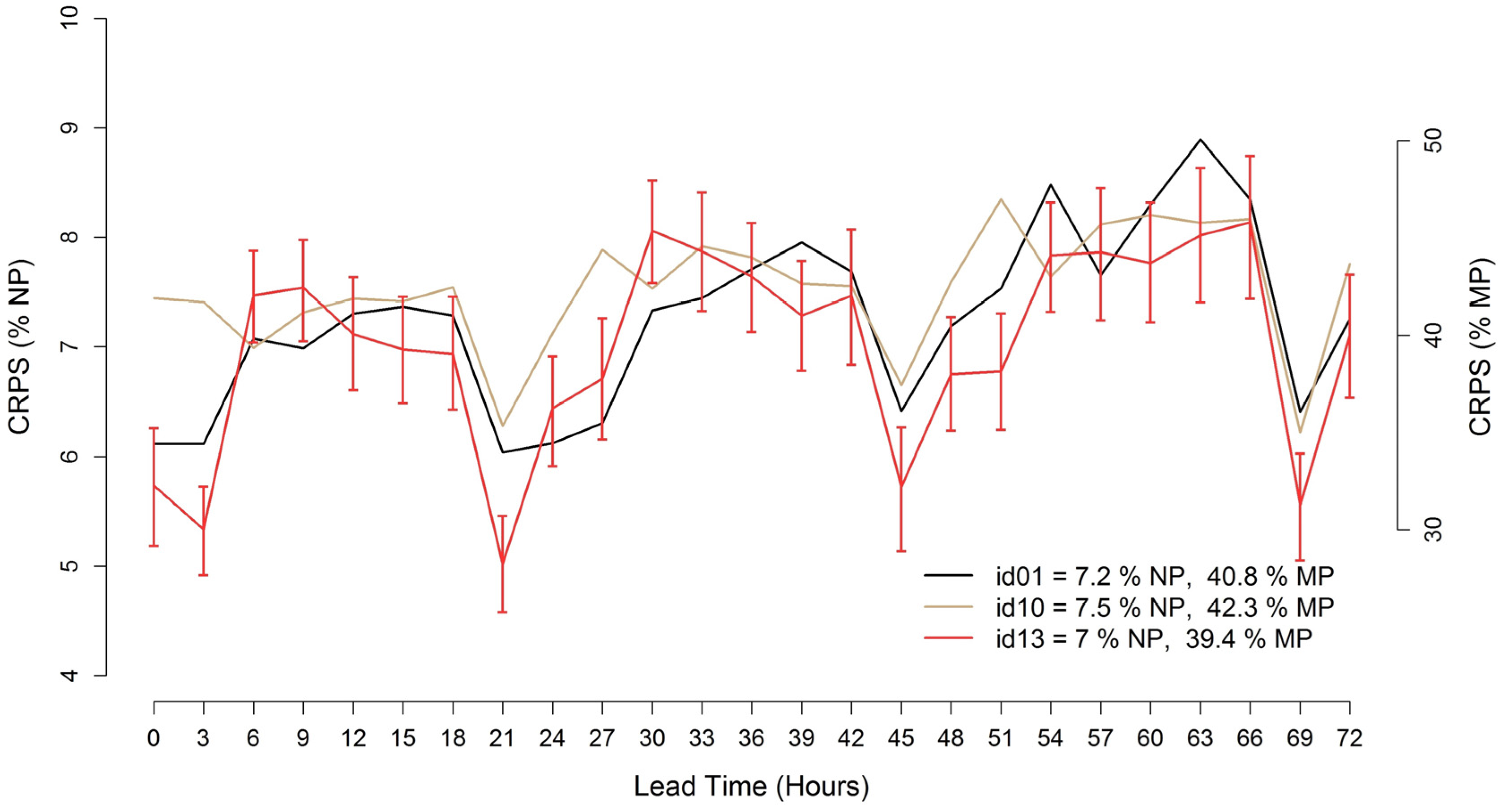
4.4. Extension to Probabilistic Wind Power Forecasts
Probabilistic forecasts were provided by a limited number of participants only for the wind test cases, in terms of quantiles of the wind power PDF for each time-step. For Abruzzo, two participants provided 19 quantiles from 5% to 95% while the third one provided nine quantiles from 10% to 90%. As previously stated, the ranking is made using the CRPS index. Rank histograms are also presented to compare statistical consistency of the different ensemble forecasts. Finally, sharpness diagrams compare the relative forecast frequencies of the different forecasts for each test case.
Figure 10 shows the
CRPS calculated at each of the 3-hourly, 0–72 h ahead time-steps for the Abruzzo case. As in the deterministic evaluation, the index is expressed as a percentage of both
NP and
MP. Looking at the diagram, the
CRPS trends of all the participants look similar. A significant diurnal cycle is evident, showing better scores during morning hours. This reflects what is observed in the deterministic evaluation. The best result, expressed as average
CRPS value over the entire 0–72 h forecast horizon, is achieved by id13 with 7.0%
CRPS/
NP and 39.4%
CRPS/
MP. Only for this trend line, bootstrap confidence bars are added in order to check for statistically significant differences between the models. It appears that, for most of the time-steps, the
CRPS of id13 is not significantly better than the other participants, in particular during the worst performance periods during night hours.
Figure 10.
Error trends of the 0–72 h ahead probabilistic wind power forecasts starting at 12 UTC for the Abruzzo test case (CRPS/NP % and CRPS/MP %).
Figure 10.
Error trends of the 0–72 h ahead probabilistic wind power forecasts starting at 12 UTC for the Abruzzo test case (CRPS/NP % and CRPS/MP %).
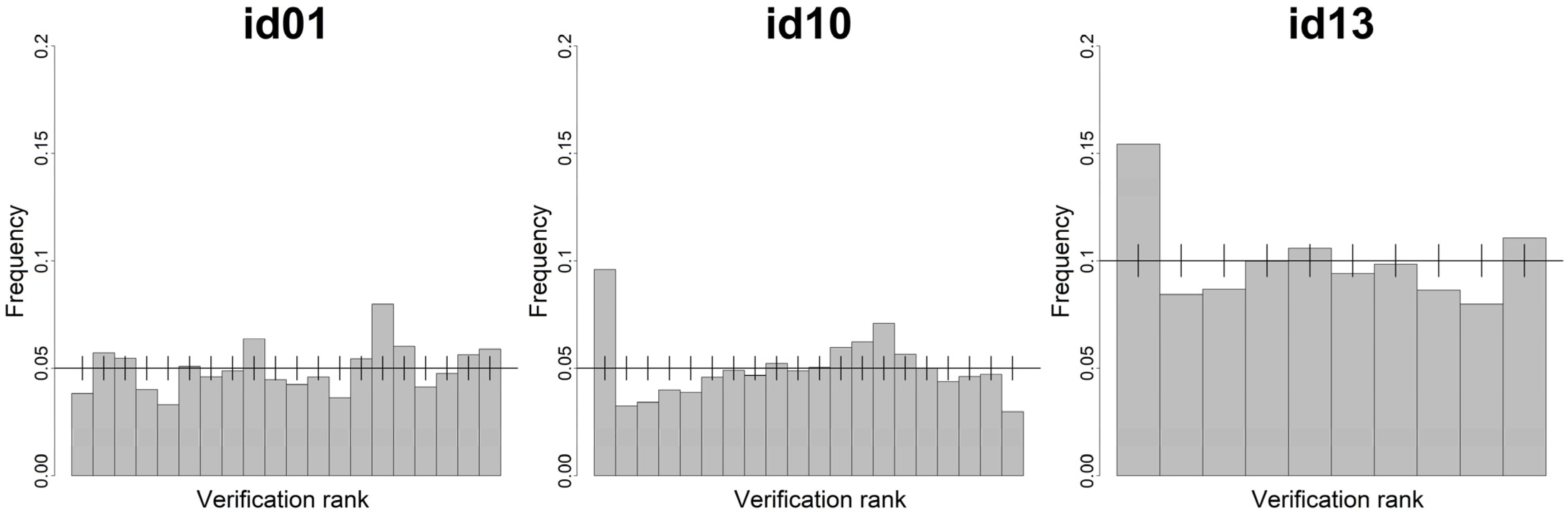
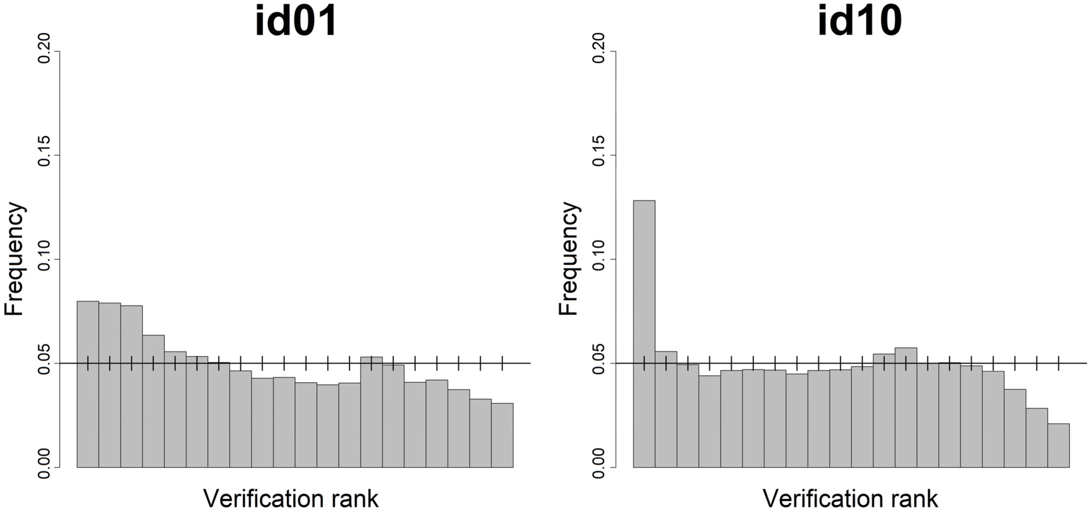
Statistical consistency is checked with the rank histograms reported in
Figure 11.
Figure 11.
Rank histograms of the 0–72 h ahead probabilistic wind power forecasts starting at 12 UTC for the Abruzzo test case.
Figure 11.
Rank histograms of the 0–72 h ahead probabilistic wind power forecasts starting at 12 UTC for the Abruzzo test case.
The different number of bins reflects the number of quantiles computed by the models: id13 delivered a wind power distribution made of 9 quantiles, while the other two participants used 19 quantiles. The vertical bars shown in the diagrams are calculated with a quantile function for a binomial distribution, in order to show a range in which deviations from the perfectly uniform distribution are still consistent with reliability. Deviations are in fact possible, since the number of samples in each bin is limited. The bars delimit the 5%–95% quantiles of the binomial distribution.
id01 shows a higher level of consistency. In fact id10 and id13 are slightly under-dispersive (i.e., over-confident) having the first and last bins more populated. In each case, it can be seen that about half of the bins with deviations from the perfect frequency still lie in the consistency range delimited by the consistency bars.
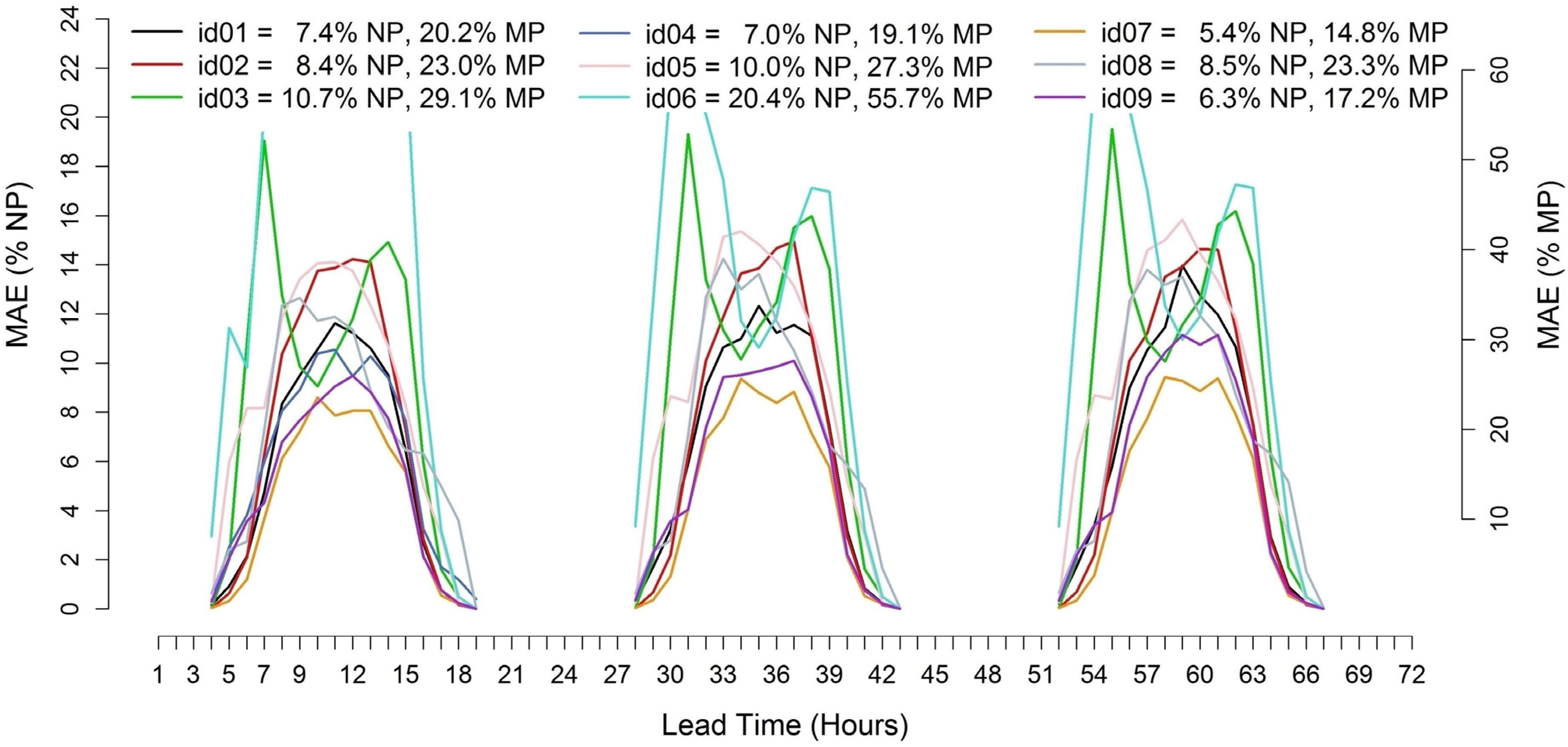
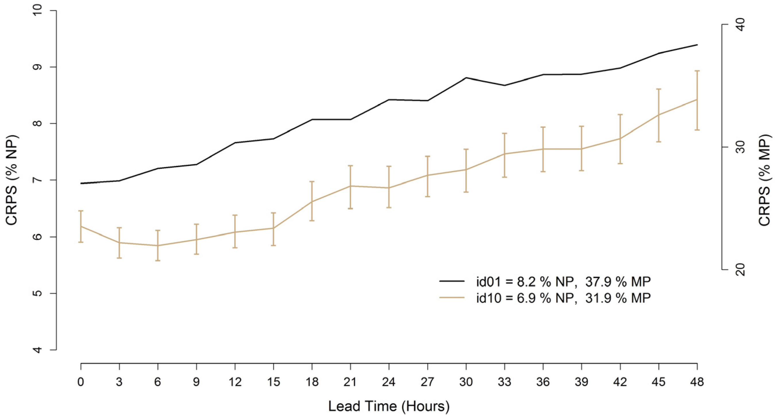
Figure 12 shows the results for the Klim test case, for which 3-hourly, 0–48 h ahead power distributions were produced. In this case id10 performs better than id01. The boot strap confidence intervals show that the differences are statistically significant for every lead time.
Figure 13 reports the rank histograms calculated for the two data sets.
Figure 12.
Error trends of the 0–72 h ahead probabilistic wind power forecasts starting at 0, 6, 12 and 18 UTC for the Klim test case (CRPS/NP % and CRPS/MP %).
Figure 12.
Error trends of the 0–72 h ahead probabilistic wind power forecasts starting at 0, 6, 12 and 18 UTC for the Klim test case (CRPS/NP % and CRPS/MP %).
Figure 13.
Rank histograms of the 0–72 h ahead probabilistic wind power forecasts starting at 0, 6, 12 and 18 UTC for the Klim test case.
Figure 13.
Rank histograms of the 0–72 h ahead probabilistic wind power forecasts starting at 0, 6, 12 and 18 UTC for the Klim test case.
Both models show a similar behavior and exhibit a positive bias. In fact, the first bins appear more populated than the others. This happens in particular for id10. However, the distribution obtained by id10 appears more consistent than that of id01 as demonstrated by the quantile bars, which maintain deviations from a uniform frequency within consistency for a greater number of bins.
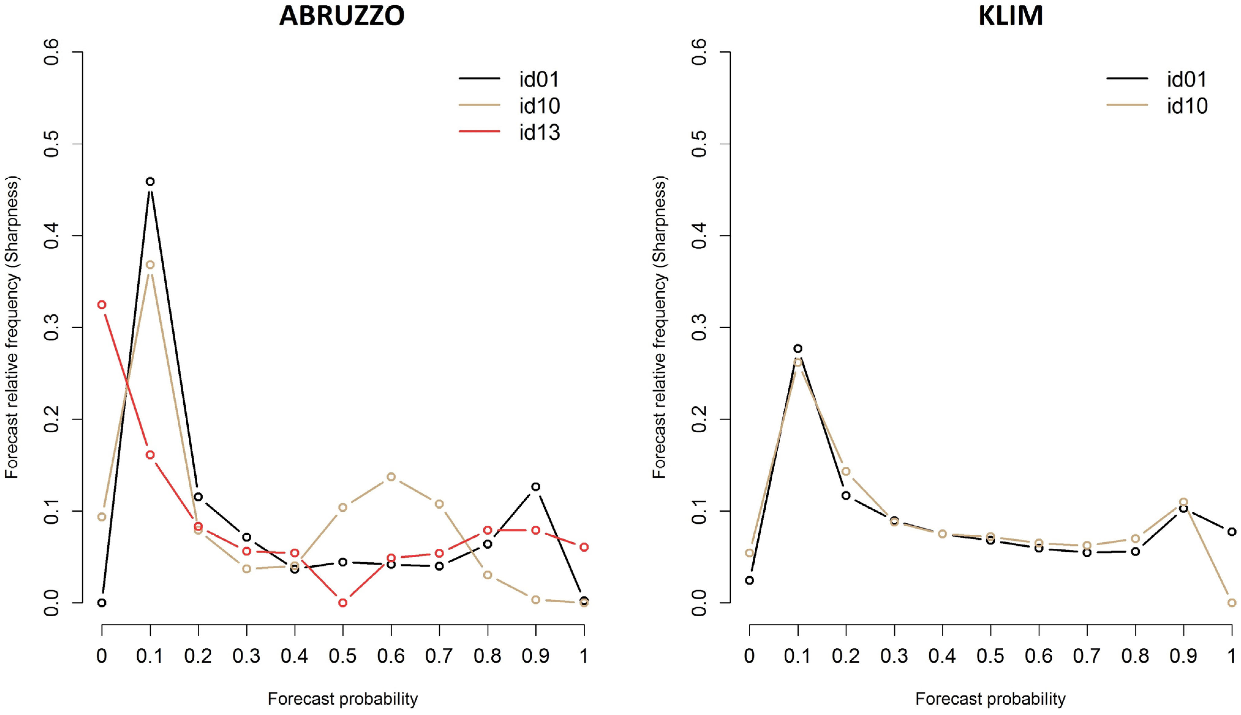
Figure 14 shows sharpness diagrams for Abruzzo and Klim respectively. In the diagrams, the average of produced power is used as threshold value.
Figure 14.
Sharpness diagrams for Abruzzo (left) and Klim (right). Mean produced power is used as threshold value.
Figure 14.
Sharpness diagrams for Abruzzo (left) and Klim (right). Mean produced power is used as threshold value.
In the case of Abruzzo, id13 shows sharper forecasts than the other participants. In fact, he is able to forecast both cases with probabilities equal to 0 and 1 with higher relative frequencies. In the case of Klim, the participants show a very similar trend. id01 behaves slightly better, in fact his relative forecast frequency for probability class equal to 1 is higher than that of id10.
The forecasting method used by id13 on Abruzzo is a local quantile regression with wind speed and wind direction as predictors [
3]. On Klim, id10 applied conditional kernel density estimation with a quantile-copula estimator, using forecasted wind speed and direction, hour of the day and forecast lead time as inputs [
33]. 5% to 95% quantiles were computed from the forecasted PDF using numerical integration.


