1. Introduction
The greenhouse gas (GHG) emission of electric power sectors around the world is about 1/3 of the total world GHG emissions, indicating the significance of the electric power sector in the global warming issue. In recent years, climate change due to GHG emissions has become a focus of international organizations and governments. In order to reduce GHG emissions, many have aimed to find more environmentally-friendly alternatives for electrical power generation. Distributed generators (DGs) are required for local energy markets, as an important alternative energy production option in the near future [
1]. DG’s technologies may include photovoltaics (PV), small wind turbines (WT), fuel cells, micro-turbines (MTs),
etc. The integration of DGs and energy storage systems (ESS) on a low voltage network is central to the concept of microgrids (MGs) [
2]. MGs can operate in either grid-connected mode or stand-alone mode [
3] and usually require an energy management strategy to ensure cooperation between the controllable units for achieving stable operation. Since MGs can result in a decrease in electricity cost, higher service reliability, an increase of energy efficiency,
etc., they are beginning to attract many utilities in the electricity market [
4,
5].
The energy management of an MG involves how to determine the most economic dispatch of the DGs that minimizes the total operating cost while satisfying the load demand and operating constraints [
6]. It is like a downsized version of the unit commitment problem that is traditionally applied to large central generators in the MG. In the grid-connected mode, the MG adjusts the power balance of supply and demand by purchasing power from the main grid or selling power to the main grid to maximize operational benefits [
7]. In the stand-alone mode, the micro-grid aims to keep a continuous power supply to customers using DG bids. One of the main constraints with DGs introduced is stability and reliability problems associated with their power scheduling [
8]. The intermittent nature of some DGs, such as wind turbines and photovoltaic systems, leads to an output that often does not suit the load demand profile. It is difficult to produce accurate day-ahead schedules in MGs. Therefore, the energy storage systems, which play an important role in MGs, allow those operations with a more flexible and reliable management of energy [
9]. They can save energy at low price hours and sell it at high price hours, which will help the network to work more efficiently and economically. Meanwhile, the operation and control in an MG will become more complicated and challenging.
The purpose of energy management of MGs is to improve energy efficiency and reduce power losses. In either grid-connected mode or stand-alone mode, an optimal scheduling of units in the energy management of MGs is carried out to maximize the benefits by operating the renewable DGs and ESS [
10,
11]. The biggest challenge comes from the intermittent nature of the renewable DGs, which is the unpredictable nature and dependence on weather and climate conditions, so that an EES is required to ensure the power demand of the load at each interval. Therefore, the operation scheduling of the dispatchable DGs in an MG is of particular concern, which can be formulated as a non-linear and mixed-integer combinatorial optimization. Various numerical techniques have been employed to address this problem [
12,
13,
14,
15,
16,
17,
18,
19,
20,
21,
22,
23,
24,
25,
26]. Mazidi
et al. [
12] proposed a two-stage stochastic objective function to solve the integrated scheduling of renewable generation and demand response programs in an MG. An energy management strategy is proposed to control an MG powered by some DGs and equipped with different storage systems: electric batteries and a hydrogen storage system [
13,
14,
15]. The authors have proposed an MG economic dispatch that can coordinate power forecasting, energy storage and energy exchanging together and then make better short-term scheduling to minimize the total operation cost [
16,
17,
18,
19]. Marzband
et al. [
20] proposed an optimal energy management system for islanded microgrids based on a multi-period artificial bee colony (MABC) algorithm and an artificial neural network combined with a Markov chain (ANN-MC) approach to predict non-dispatchable power generation and load demand, while taking uncertainties into account. An operational architecture for real-time operation (RTO) is proposed to run the MG in islanded mode, ensuring uninterruptable power supply services and reducing cost [
21]. Marzband
et al. [
22] proposed an energy management system (EMS) algorithm based on mixed-integer nonlinear programming (MINLP) for MGs in islanded mode in different scenarios. A model for optimal energy management with the goal of cost and emission minimization is presented based on the operation strategies of the hybrid DGs [
23,
24]. Some artificial intelligent techniques have been presented to solve the economic dispatch of MGs and have shown their effectiveness [
25,
26,
27,
28,
29]. The common disadvantages of the above methods are their long computation times and the lack of guarantee that a global optimal solution can be found. In order to overcome the local optima problem, an enhanced bee colony optimization (EBCO) algorithm is proposed in this paper.
Bee colony optimization (BCO), unlike most population-based algorithms, employs different moving patterns to research the feasible solution space [
30]. The BCO algorithm is improved by referring to genetic algorithm (GA), evolutionary programming (EP) and particle swarm optimization (PSO) for strengthening the optimization of parameter control and population evolution. The BCO has many of the advantages of biological intelligence in searching, but it has the shortcoming of easy and rapid convergence in computation and poor stability in higher dimensional search. The energy management of MGs is a complex and high-dimensional problem with multiple constraints. In this paper, therefore, an EBCO algorithm is proposed to address this problem. In the EBCO procedure, the self-adaption and repulsion factors are embedded in the bee swarm of BCO in order to improve the behavior patterns of each bee swarm and to increase its search efficiency and accuracy in high dimensions. Different modifications in moving patterns of EBCO are proposed to search the feasible space more effectively. EBCO is intended to significantly improve the efficiency of MG energy production and to optimize the use of existing DGs to maximize profit. The effectiveness of the algorithm is demonstrated by performing optimization on several cases, and the results are compared to those in previous publications. Our results show that the proposed method is feasible, robust and more effective than many previously-developed algorithms.
3. Problem Formulation
The energy operation management in a typical MG can be defined as an optimization function, which minimizes the total operating cost while satisfying the equality and inequality constraints. The objective function and associated constraints of the problem can be formulated as follows:
The constraints include both the system constraints and the unit’s constraints and involve:
(2) Unit power generation limitation:
(3) Minimum up-time constraint:
(4) Minimum down-time constraint:
(7) Interchange with utility constraints:
(8) The capacity constraints for the battery:
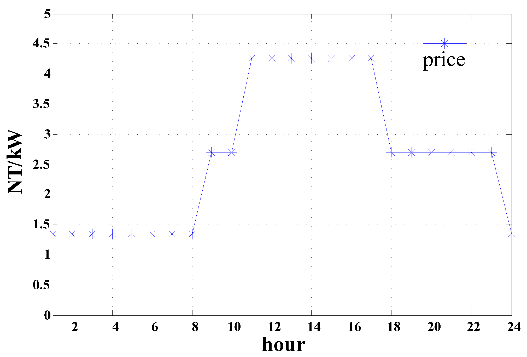
Figure 2 shows the electricity price in a day [
33].
Figure 2.
The time-of-use (TOU) rate in a day.
Figure 2.
The time-of-use (TOU) rate in a day.
4. Enhanced Bee Colony Optimization
Bee colony optimization (BCO) was developed by [
30] for numerical optimization in 2005. This algorithm mimics the food foraging behavior of honey bees. In the EBCO algorithm, the swarm also consists of three categories, scout bees, employed bees and onlooker bees. They carry out various activities to sustain the hive life. The scout bees perform a random search for new food sources, and employed bees have the role of exploiting the identified food sources and sharing the various pieces of information with onlooker bees waiting in the hive to make a better decision. The EBCO includes the following phases: initialization, employed bee phases, onlooker bee phases and scout bee phases. The EBCO can be described as follows.
4.1. Initial Solutions
The initial parameters in the EBCO are the number of food sources (NFS), which is equal to the bees. The initial population of solutions is filled with the NFS number of randomly-generated food sources in a limited area. The random positions of food sources are generated by the following equation:
is the
i-th population of solution vector
j-th and
NFS is set to 50.
and
represent the lower and upper boundaries of solution vector
j-th.
rand is a uniformly-distributed random number in the range of (0, 1). The fitness function is defined as:
is the objective function.
and
are the equality and inequality constraints.
M and
N are the numbers of equality and inequality constraints.
and
are the penalty factors that can be adjusted in the optimization procedure.
is defined by:
If one or more variables violate their limits, the penalty factors will increase, and the corresponding individual will be rejected to avoid generating an infeasible solution.
4.2. Employed Bees
In the BCO, based on the behavior of the bees, a hard restriction exists on the flying pattern of bees. BCO may cause premature convergence by using the information achieved by a swarm imperfectly. In the EBCO, the better part of the employed bees fly considering the social and cognitive information achieved by the swarm. Each bee knows its current optimal position (
), which is analogous to the personal experiences of each particle. Each bee also knows the current global optimal position (
) among all bees in the population. EBCO can have several solutions at the same time, and particles have a cooperative relationship for sharing messages. In other words, it tries to reach compatibility between local search and global search. At this stage, each employed bee makes a change on the position of food sources to generate a new food sources in the neighborhood of its present position as follows:
where
rand is the random numbers between zero and one.
k is a randomly-chosen index, and
.
and
are the initial acceleration constants.
and
are the final acceleration constants.
is the maximal iteration, and
is the current iteration.
is the concept of the interference factor.
,
,
,
and
are set to 1.5, 0.5, 0.5, 1.5 and 200, respectively.
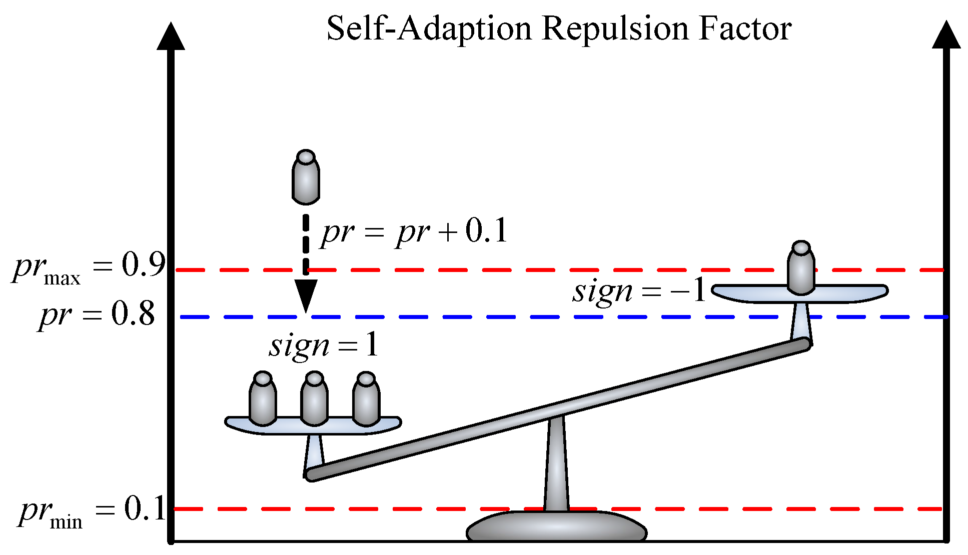
In the EBCO, a self-adaption repulsion factor is introduced to further strengthen the global search capability of BCO. This factor can fly over some parts of the search space and may include profitable information by the bee swarm. The increasing diversity of a bee swarm is incorporated in order to avoid premature convergence. To enlarge the search area that might have been neglected, the concept of the interference factor,
, is introduced in Equation (22):
Its initial setting is . When the randomly-generated rand is larger than the predefined pr, a reverse search, as given in Equation (22), will take place. sign is the self-adaption repulsion factor. The sign values used by bee swarms are recorded, and the pr value is based on self-adaption repulsion, which is adjusted according to the fitness value in each iteration. In this paper, set prmax = 0.9 and prmin = 0.1. The searching procedure is described as follows (Algorithm 1):
| Algorithm 1 Self-adaption repulsion factor search |
| 1: if comes from |
| 2: |
| 3: if then and |
| 4: else |
| 5: if then and |
| 6: else comes from |
| 7: |
| 8: if then and |
| 9: else |
| 10: if then and |
| 11: end |
If in the current iteration, the optimal fitness value is generated at
, let
to increase the probability of positive feedback for each bee swarm, as shown in
Figure 3. Conversely, if in the current iteration, the optimum fitness value is generated at
, the probability of negative feedback should be increased.
is the number of iterations in this procedure.
is the upper limit of
, and
. After,
is continuously maintained at the maximum or minimum values for
times and meets. The updated food sources are used in this study to improve the diversity of the solutions, and this behavior is referred to as the self-adaption repulsion factor.
Figure 3.
Probability variation of pr.
Figure 3.
Probability variation of pr.
4.3. Onlooker Bees
The onlooker bees in the improved bee swarm algorithm will follow the employed bees to obtain nectar information. Instead of joining the group of employed bees, the onlooker bee will only follow. The flying path of the onlooker bees is modified by using the probabilistic selection method, as shown in Equation (23), to follow the employed bees. In the working mode of the onlooker bees, the repulsive force is also included in order to enlarge the search area, as shown in Equation (24).
where
is the better fitness value of the food source and
is the number of employed bees.
is the number of onlooker bees.
4.4. Scout Bees
In the EBCO, the model of the scout bees will no longer be a baseless random search. The working model of the scout bees was modified to the average value of the global optimum solution and all swarm locations. After comparison, the new location of scout bees is generated by Equation (25):
where variable
ns is the number of scout bees and
mean is the average of all variable solutions in the
t-th iteration. The population size for employed bees, onlooker bees and scout bees are 20, 20 and 10, respectively.
4.5. Stop Condition
The terminating condition is the maximal number of iterations. If the preset target is not yet attained, then go back to
Section 4.2 and repeat the operation.
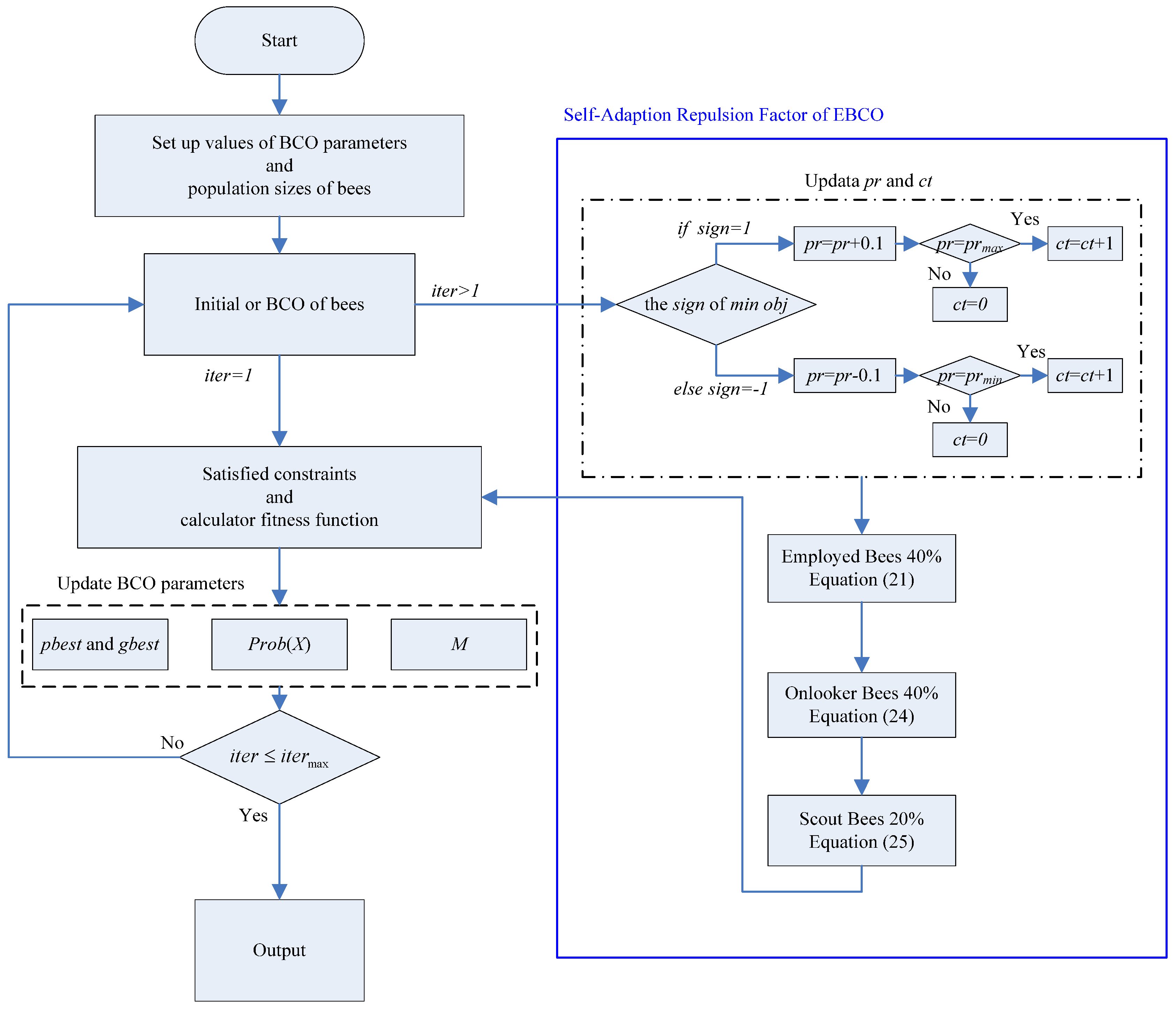
Figure 4 shows the flowchart of EBCO.
Figure 4.
The flowchart of enhanced bee colony optimization (EBCO).
Figure 4.
The flowchart of enhanced bee colony optimization (EBCO).
5. Case Studies
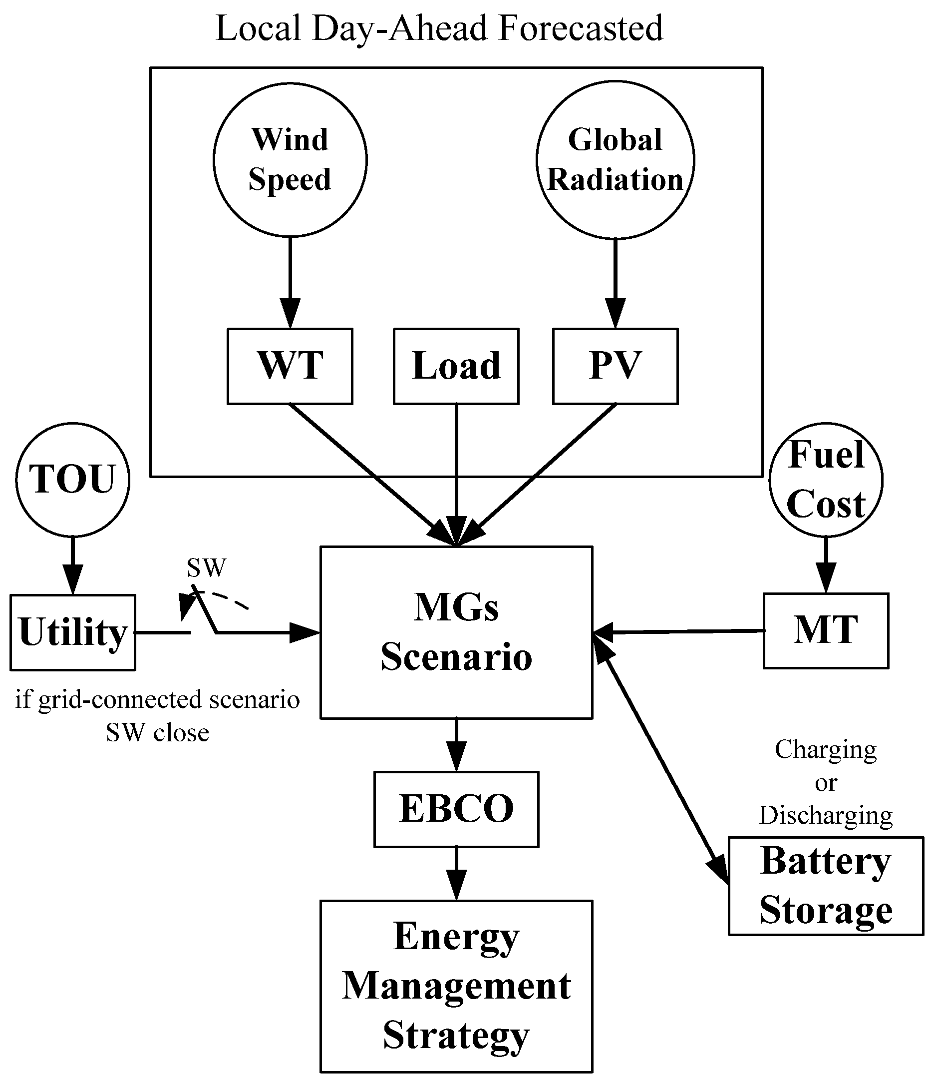
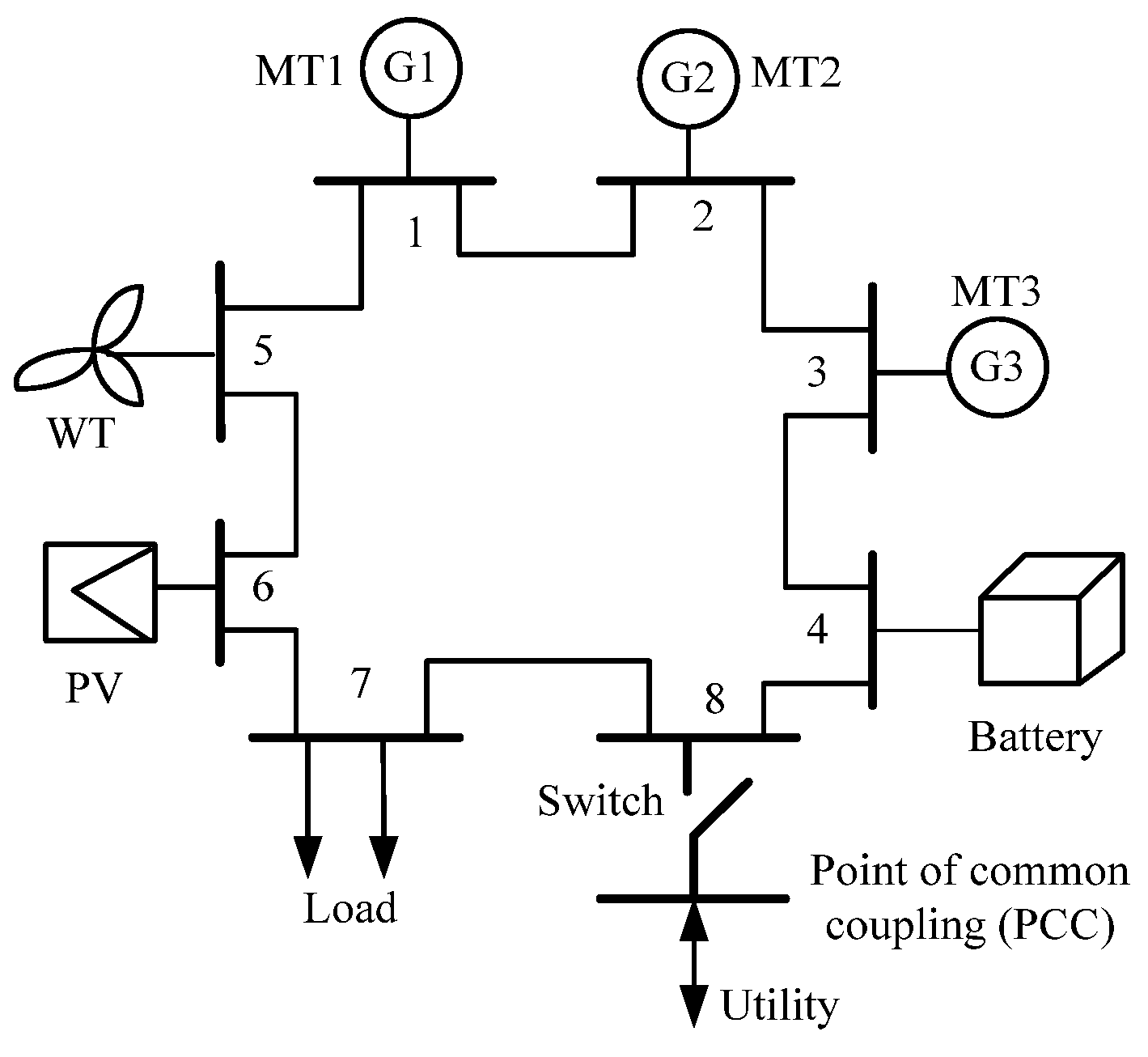
In this paper, a typical low voltage MG is considered as the test system for the application of the proposed methodology, as shown in
Figure 5 [
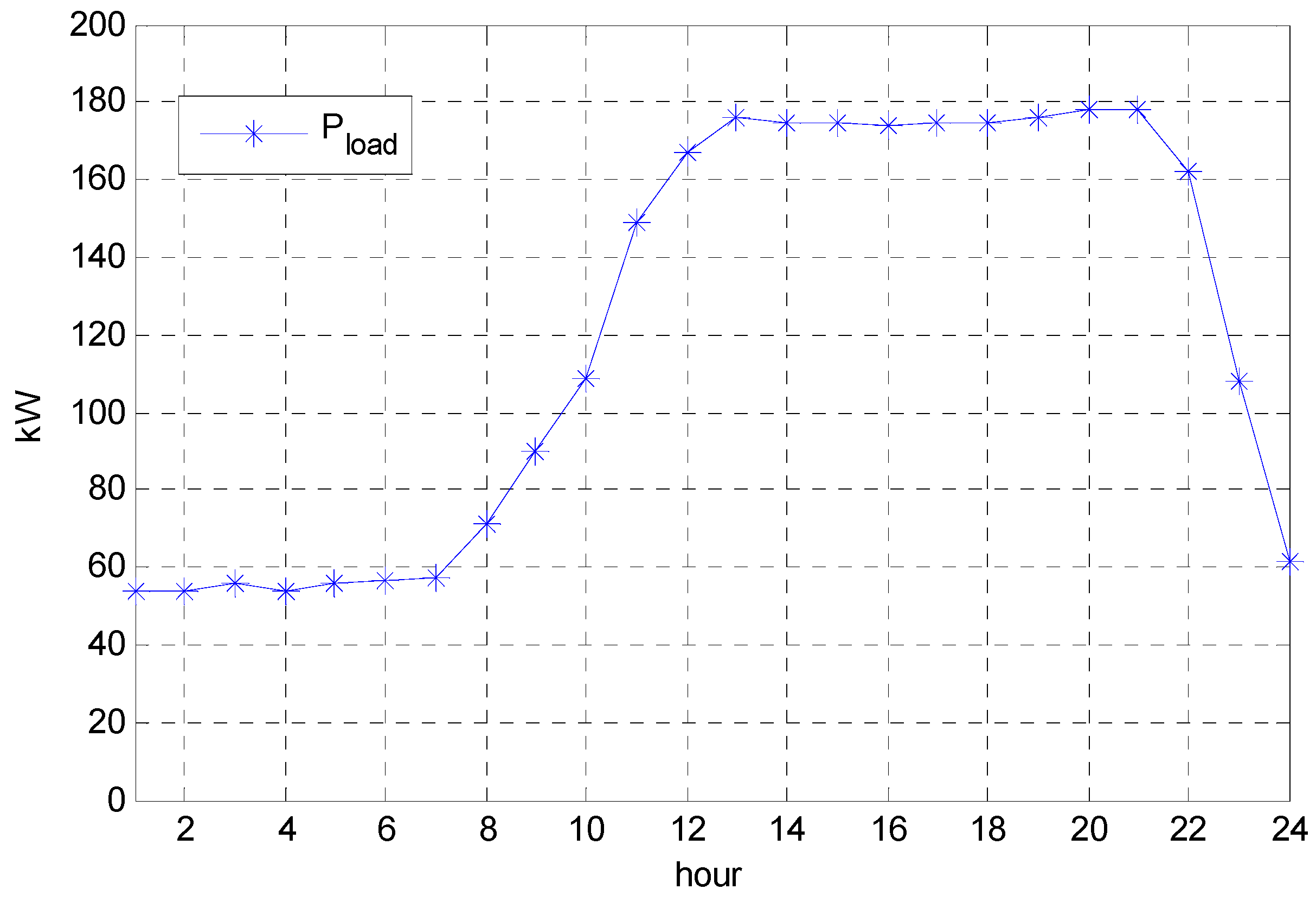
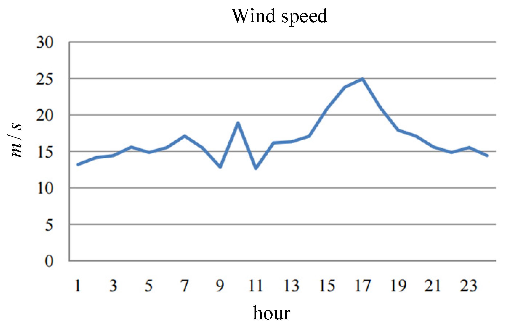
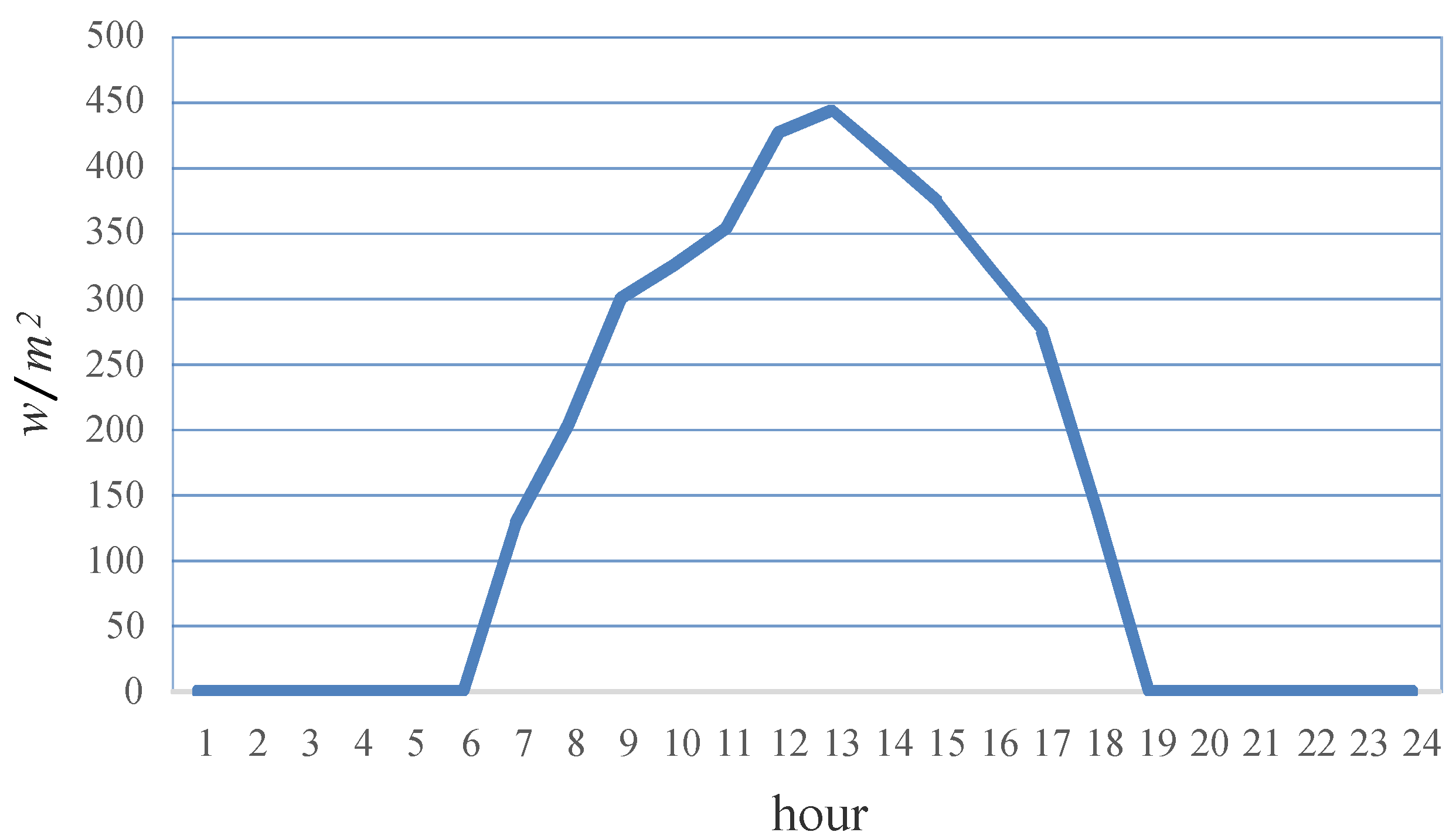
34]. The configuration of the MG system consists of a set of DG units, including three MTs, a WT, a PV and battery storage. The system is exchanged with the utility from the point of common coupling (PCC). The total load demand, the forecasted wind speed of the WT and the forecasted global radiation of the PV in a typical day is shown in
Figure 6,
Figure 7 and
Figure 8. It should be noted that a time period of one day with an hourly time step is considered in this study. All DGs produced the active power at the unity power factor.
Figure 5.
The diagram of a typical low-voltage MG system.
Figure 5.
The diagram of a typical low-voltage MG system.
Figure 6.
Load demand in a typical day.
Figure 6.
Load demand in a typical day.
Figure 7.
The forecasted wind speed of the WT in a typical day.
Figure 7.
The forecasted wind speed of the WT in a typical day.
Figure 8.
The forecasted global radiation of the PV in a typical day.
Figure 8.
The forecasted global radiation of the PV in a typical day.
5.1. Results at Different Scenarios
In order to analyze and compare the performance of the MG system in the different scenarios, two scenarios were simulated; a grid-connected situation and a stand-alone scenario. In a grid-connected scenario, the cost-benefit power trading between the MG system and the utility can be used at any time. In a stand-alone scenario, demand side management considered the power balance, which means to meet load demand by using DGs, WT, PV and battery storage. In both scenarios, there is a high penetration level of DGs with a larger power fluctuation.
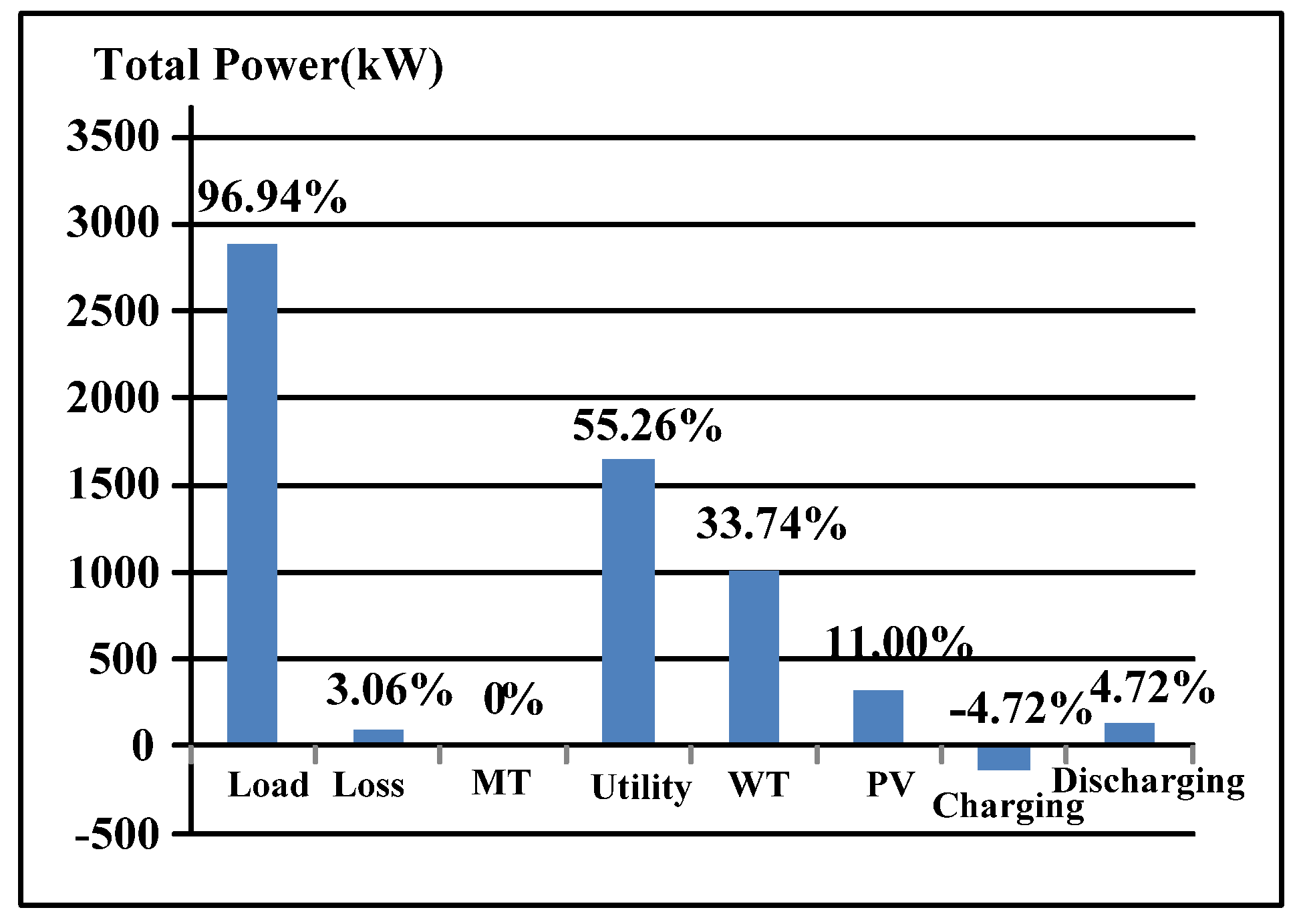
Figure 9 shows the generation supply scheme in the grid-connected scenario. The generation supplied by the DG’s units and utility units is 44.74% and 55.26% of total generation, and the loss is 3.06%. The MG is self-sufficient to meet the load demand, and the power from the WT and PV meet about 45.89% of the load demand. If the system supplied all power from the utility, the total cost is about NT$8305.235. The power from the PV and WT meet most load demand; the cost can be cut down to NT$5521.03. With the cooperation of the battery and other MTs, the cost is reduced to NT$5037.031 through the control sequence determined by optimizing dispatch. It is noted that the production cost of MTs is greater than that of the electricity purchased from the utility.
Figure 9.
The generation supply scheme in the grid-connected scenario.
Figure 9.
The generation supply scheme in the grid-connected scenario.
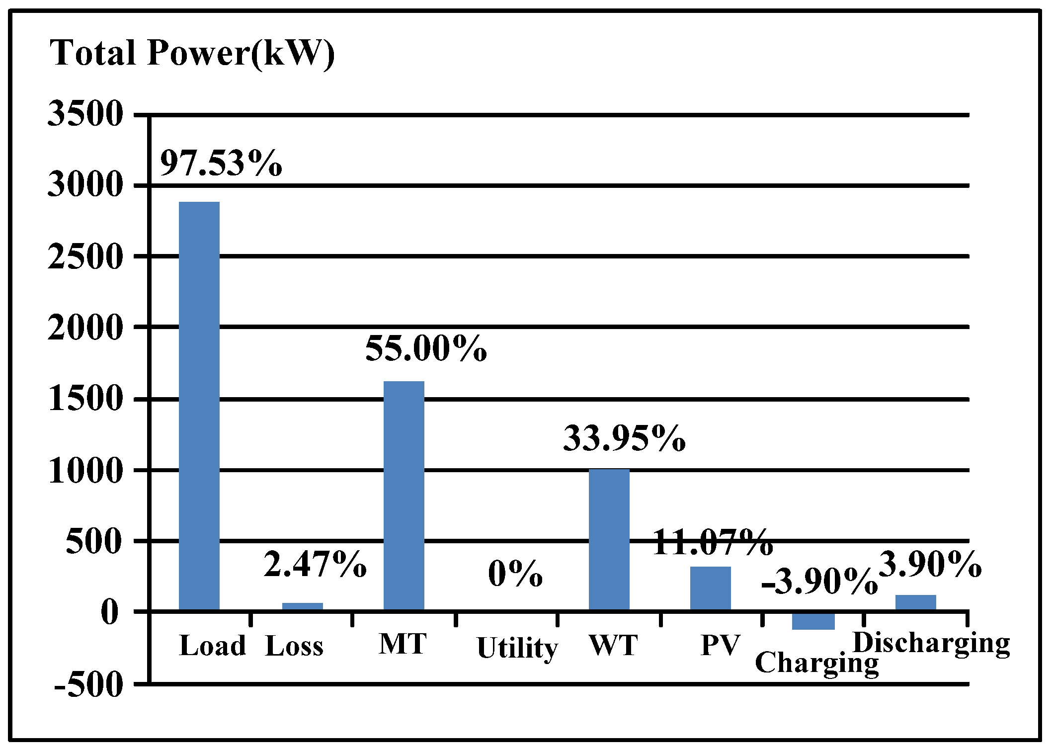
Figure 10 shows the generation supply scheme in the stand-alone scenario. The generation supplied by MT units, the WT and the PV is 55.0%, 33.95% and 11.07% of total generation, respectively. The loss is reduced from 3.06% to 2.47%. Since the power from the utility is broken down in the stand-alone scenario, the MTs must produce more power to meet the load demand. In the stand-alone scenario, half of the electricity is generated by MTs.
Figure 10.
The generation supply scheme in the stand-alone scenario.
Figure 10.
The generation supply scheme in the stand-alone scenario.
Table 1 shows the simulation results with different scenarios. 100 test runs are conducted for each scenario. From
Table 1, it can be seen that the proposed algorithm offers good performance in terms of searching solution, number of generations to convergence and the average execution time. The average execution time for two cases is only 0.78 and 2.45 s, respectively. It is obvious that the EBCO can solve the problem efficiently and often achieve a fast and global or near global optimal solution.
Table 1.
Simulation results of the test systems.
Table 1.
Simulation results of the test systems.
| Item | Grid-Connected Scenario | Stand-Alone Scenario |
|---|
| Best (NT$) | 5037.031 | 15,925.274 |
| Worst (NT$) | 5048.385 | 15,951.841 |
| Average (NT$) | 5041.457 | 15,936.813 |
| Average number of generations to converge | 150 | 173 |
| Number of trials reaching optimum | 63 | 46 |
| Average execution time (s) | 0.78 | 2.42 |
5.2. Convergence Test
Table 2 shows the comparisons of EP [
26], GA [
27], PSO [
25], BCO [
30] and EBCO during different scenarios. The tests are carried out on a P-IV, Core 2 Duo 2.4 Hz, 2.0 GHz CPU and 4 GB DRAM memory. From
Table 2, the improvement of the EBCO over other algorithms is clear.
Figure 11 and
Figure 12 illustrate the convergence characteristics of EP, GA, PSO, BCO and EBCO in the grid-connected scenario and stand-alone scenario. This also shows the capacity of EBCO to explore a more likely global optimum.
Table 2.
Comparison of the evolutionary programming (EP), genetic algorithm (GA), particle swarm optimization (PSO), bee colony optimization (BCO) and enhanced bee colony optimization (EBCO) algorithms.
Table 2.
Comparison of the evolutionary programming (EP), genetic algorithm (GA), particle swarm optimization (PSO), bee colony optimization (BCO) and enhanced bee colony optimization (EBCO) algorithms.
| Algorithms | Grid-Connected Scenario (NT$) | Stand-Alone Scenario (NT$) |
|---|
| EP | 5049.711 | 17,153.754 |
| GA | 5045.813 | 16,958.279 |
| PSO | 5038.196 | 16,224.526 |
| BCO | 5038.209 | 16,122.949 |
| EBCO | 5037.030 | 15,925.270 |
Figure 11.
The convergence characteristics of EP, GA, PSO, BCO and EBCO in the grid-connected scenario.
Figure 11.
The convergence characteristics of EP, GA, PSO, BCO and EBCO in the grid-connected scenario.
Figure 12.
The convergence characteristics of EP, GA, PSO, BCO and EBCO in the stand-alone scenario.
Figure 12.
The convergence characteristics of EP, GA, PSO, BCO and EBCO in the stand-alone scenario.
5.3. Robustness Test
All mentioned algorithms were also tested in the grid-connected scenario and stand-alone scenario with the results shown in
Table 3 and
Table 4. Each algorithm was executed by 100 trials with the same initial parents. It can be seen that EBCO improves the searching performance, with the best probability of guaranteeing a global optimum. From
Table 3 and
Table 4, the EBCO algorithm demonstrates better accuracy, while the number of trials reaching the optimum is greater than those in EP, GA, PSO and BCO. Although the average execution time is also much lesser than that of GA and slightly higher than those of EP, PSO and BCO, the average number of generations to converge is only 150. The practical execution time of EBCO is thus lower than those of other algorithms.
Table 3.
Robustness test for the EP, GA, PSO, BCO and EBCO algorithms in the grid-connected scenario.
Table 3.
Robustness test for the EP, GA, PSO, BCO and EBCO algorithms in the grid-connected scenario.
| Algorithm | Maximal Converged Cost (NT$) | Minimal Converged Cost (NT$) | Average Converged Cost (NT$) | Average Number of Generations to Converge | Number of Trials Reaching Optimum | Average Execution Time (s) |
|---|
| EP | 5074.095 | 5049.711 | 5060.149 | 191 | 4 | 0.56 |
| GA | 5067.188 | 5045.813 | 5054.248 | 193 | 6 | 1.53 |
| PSO | 5053.567 | 5038.209 | 5047.794 | 190 | 45 | 0.67 |
| BCO | 5051.554 | 5038.196 | 5046.624 | 169 | 42 | 0.72 |
| EBCO | 5048.385 | 5037.030 | 5041.457 | 150 | 64 | 0.78 |
Table 4.
Robustness test for the EP, GA, PSO, BCO and EBCO algorithms in the stand-alone scenario.
Table 4.
Robustness test for the EP, GA, PSO, BCO and EBCO algorithms in the stand-alone scenario.
| Algorithm | Maximal Converged Cost (NT$) | Minimal Converged Cost (NT$) | Average Converged Cost (NT$) | Average Number of Generations to Converge | Number of Trials Reaching Optimum | Average Execution Time (s) |
|---|
| EP | 17,382.375 | 17,153.754 | 17,266.188 | 197 | 1 | 1.68 |
| GA | 17,186.573 | 16,958.279 | 17,010.570 | 198 | 2 | 5.94 |
| PSO | 16,391.596 | 16,224.526 | 16,286.286 | 191 | 26 | 2.18 |
| BCO | 16,279.849 | 16,122.949 | 16,164.635 | 187 | 31 | 2.23 |
| EBCO | 15,951.841 | 15,925.270 | 15,936.813 | 173 | 46 | 2.42 |


