Abstract
Nuclear and other large-scale energy-producing plants must include systems that guarantee the safe discharge of residual heat from the industrial process into the atmosphere. This function is usually performed by one or several cooling towers. The amount of heat released by a cooling tower into the external environment can be quantified by using a numerical simulation model of the physical processes occurring in the respective tower, augmented by experimentally measured data that accounts for external conditions such as outlet air temperature, outlet water temperature, and outlet air relative humidity. The model’s responses of interest depend on many model parameters including correlations, boundary conditions, and material properties. Changes in these model parameters induce changes in the computed quantities of interest (called “model responses”), which are quantified by the sensitivities (i.e., functional derivatives) of the model responses with respect to the model parameters. These sensitivities are computed in this work by applying the general adjoint sensitivity analysis methodology (ASAM) for nonlinear systems. These sensitivities are subsequently used for: (i) Ranking the parameters in their importance to contributing to response uncertainties; (ii) Propagating the uncertainties (covariances) in these model parameters to quantify the uncertainties (covariances) in the model responses; (iii) Performing model validation and predictive modeling. The comprehensive predictive modeling methodology used in this work, which includes assimilation of experimental measurements and calibration of model parameters, is applied to the cooling tower model under unsaturated conditions. The predicted response uncertainties (standard deviations) thus obtained are smaller than both the computed and the measured standards deviations for the respective responses, even for responses where no experimental data were available.
1. Introduction
Nuclear and other energy-producing large-scale industrial installations must include systems that guarantee the safe discharge of residual heat from the industrial process into the atmosphere. In the case of nuclear power plants, the residual heat is discharged into the atmosphere by using cooling towers. The amount of heat released into the external environment can be quantified by using a numerical simulation model of the physical processes that take place within the respective cooling tower, complemented by experimentally measured data that characterize external conditions such as outlet air temperature, outlet water temperature and outlet air relative humidity. Based on the flow regime occurring in the fill section, the cooling towers are generally divided in two categories: cross-flow towers and counter-flow towers. A model for the steady-state simulation of both cross-flow and counter-flow wet cooling towers has been presented in [1]. The natural draft cooling tower model presented in [1] was validated against experimental data in [2,3] under partially and totally saturated conditions. This work also analyses a natural draft cooling tower, but, in contradistinction with the work in [2,3], the draft cooling tower analyzed in this work operates always under unsaturated conditions. Thus, just as in [2,3], the cooling tower analyzed in this work is operated with the tower’s fan turned off, causing the air mass flow rate to be an unknown state variable to be determined by solving the underlying set of governing equations. In contradistinction to [2,3], however, the unsaturated operating conditions analyzed in this work are modeled by governing equations that differ from the ones presented in [2,3].
The work in [2,3] used a considerably more accurate and efficient numerical method than was used in [1], thereby overcoming all of the non-convergence issues that had plagued some of the computations in [1]. The accurate and efficient numerical method introduced in [2,3] is also used in this work for computing the following quantities: (i) The water mass flow rates at the exit of each control volume along the height of the fill section of the cooling tower; (ii) The water temperatures at the exit of each control volume along the height of the fill section of the cooling tower; (iii) The air temperatures at the exit of each control volume along the height of the fill section of the cooling tower; (iv) The humidity ratios at the exit of each control volume along the height of the fill section of the cooling tower; (v) The air relative humidity at the exit of each control volume; and (vi) the air mass flow rate at the outlet of the cooling tower.
This work is organized as follows: Section 2 presents the mathematical model of a mechanical draft counter-flow cooling tower operating under unsaturated conditions, along with the numerical solution for the quantities (state functions) mentioned above in items (i) through (vi). Section 3 presents the development of the adjoint sensitivity model for the counter-flow cooling tower operating under unsaturated conditions using the general adjoint sensitivity analysis methodology (ASAM) for nonlinear systems [4,5,6]. Using a single adjoint computation enables the efficient and exact computation of the sensitivities (functional derivatives) of the model responses to all of the 47 model parameters, thus alleviating the need for repeated forward model computations in conjunction with finite difference methods. Sensitivities are subsequently used for ranking the contributions of the single model parameters to the model responses variations, computing the propagated uncertainties of the model responses, and for the application of the “predictive modeling for coupled multi-physics systems” (PM_CMPS) methodology [7], aimed at yielding best-estimate predicted nominal values and uncertainties for model parameters and responses.
Section 4 presents the results of applying the PM_CMPS methodology, which simultaneously combines all of the available computed information and experimentally measured data for the buoyancy-operated counter-flow cooling tower operating under unsaturated conditions. The best-estimate results predicted by the PM_CMPS methodology reveal that the predicted values of the standard deviations for all the model responses, even those for which no experimental data have been recorded, are smaller than either the computed or the measured standards deviations for the respective responses. After discussing the significance of these predicted results, this work concludes by indicating possible further generalizations of the adjoint sensitivity analysis and PM_CMPS methodologies.
2. Mathematical Model of a Mechanical Draft Counter-Flow Cooling Tower Operating under Unsaturated Conditions
The experimental measurement used for this study have been performed at Savannah River National Laboratory (SRNL) for F-Area Cooling Towers in the period going from April, 2004 to August, 2004; this data collection comprises a total of 8079 benchmark data sets [8], each one containing the following (four) measured quantities: (i) Exhaust air temperature according to the “Tidbit” sensor, which will be denoted in the following as ; (ii) Exhaust air temperature according to the “Hobo” sensor, which will be denoted in the following as ; (iii) Outlet water temperature, which will be denoted in the following as ; (iv) Exhaust air relative humidity, which will be referred to as . For a data set to be intended as unsaturated is required that the value of the exhaust air relative humidity , computed by making use of the SNRL simulation code CTTool [1], is smaller than 100%, while the threshold is set on correspondence of the saturation line . With this standard set, 6717 data sets among the total 8079 measured have matched the requirement above and have been therefore identified as “unsaturated”, leading to include them in the present study. Histogram plots and analyses of the statistical moments of the selected 6717 data sets have been gathered in Appendix A. The state functions chosen for the analysis of the cooling tower mathematical model hereby considered have been selected according to the quantities comprised in the experimentally measured data sets. A numerical method, which has been presented in detail in [2], has been implemented to improve both the accuracy and the efficiency in the solution of the constitutive equations system governing the counter-flow cooling tower model.
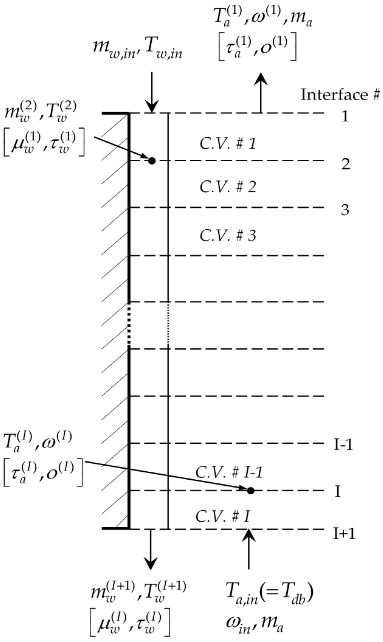
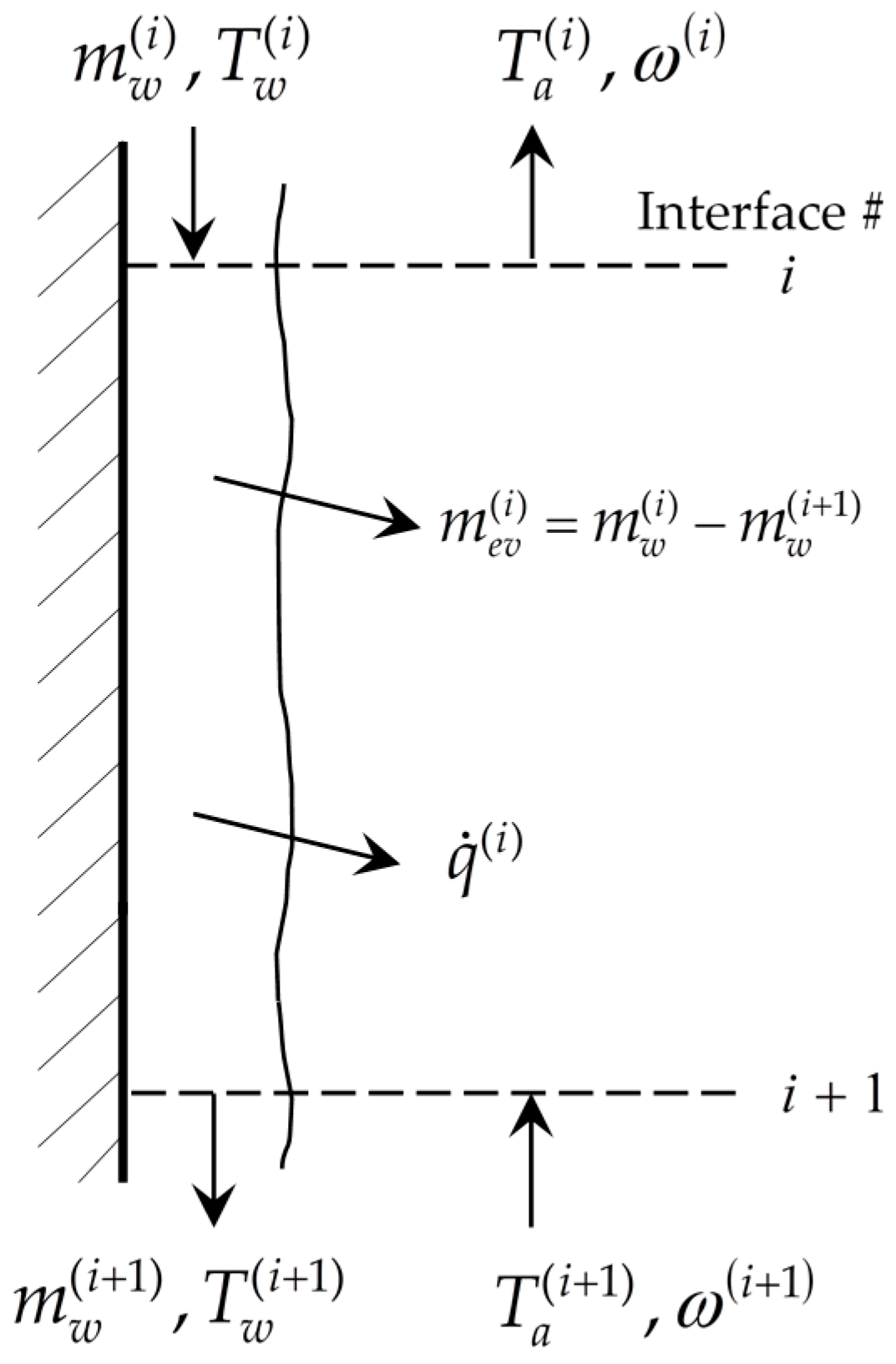
The cooling tower model analyzed in this work has been originally presented in [1] and has been thoroughly described in [2], from which Figure 1, Figure 2 and Figure 3 have been taken. Natural draft air enters the tower just below the fill section, through which it passes flowing upwards along the height of the tower finally exiting at the top, through an exhaust comprising a fan. Inlet water enters the tower below the drift eliminator, and is sprayed downwards over the fill section, leading to the creation of a uniform film flow through the fill.
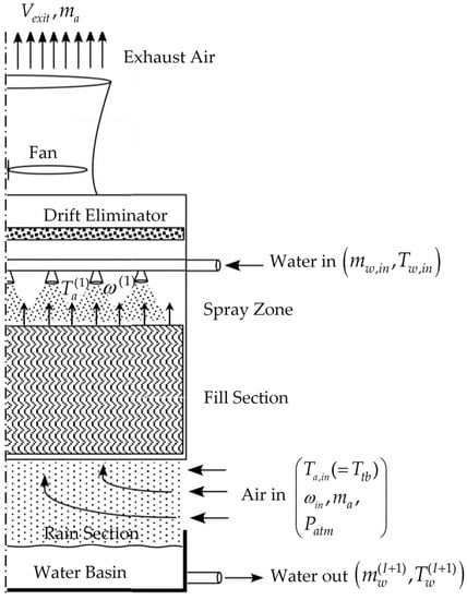
Figure 1.
Flow through a counter-flow cooling tower.
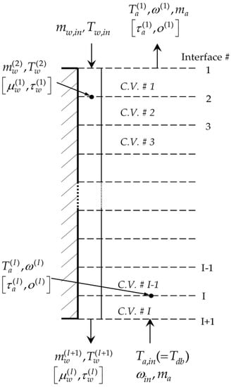
Figure 2.
Fill section nodalization comprising 49 control volumes ; both the forward state functions and the adjoint state functions selected are shown in the picture.
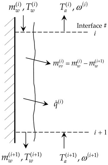
Figure 3.
Heat and mass transfer phenomena at the interface between downward water film and upward air within a single control volume of the cooling tower’s fill section.
The magnitude of the heat and mass transfer processes occurring in the counter-flow cooling tower of interest can be mathematically determined by obtaining the solution of the nonlinear system comprising the following balance equations: (A) Liquid continuity; (B) Liquid energy balance; (C) Water vapor continuity; (D) Air/water vapor energy balance; (E) Mechanical energy balance. In the derivation process of these equations, the cooling tower model has undergone several assumptions, such as:
- air and water stream temperatures are uniform at any cross section;
- the cross-sectional area of the cooling tower is assumed to be uniform;
- the heat and mass transfer only occur in the direction normal to flows;
- the heat and mass transfer through tower walls to the environment is neglected;
- the heat transfer from the cooling tower fan and motor assembly to the air is neglected;
- the air and water vapor is considered a mixture of ideal gasses;
- the flow between flat plates is unsaturated through the fill section.
It is worth specifying that this work applies to cooling towers of moderate size, for which it is possible to neglect the occurrence of the heat and mass transfer phenomena in the rain section. Figure 2 displays the vertical nodalization chosen for the fill section. Figure 3 offers a more detailed description of the heat and mass transfer processes occurring at the interface between the water film and the air flow within a single control volume.
As reminded above, when the cooling tower is operated in natural draft/wind-aided mode the mass flowrate of dry air becomes an additional unknown. Even with the fan off though, hot water flowing through the cooling tower will cause air to continue to flow through the tower due to buoyancy, with possible flow enhancements caused by the wind pressure at the air inlet to the cooling tower. The state functions underlying the cooling tower model (cf., Figure 1, Figure 2 and Figure 3) are as follows:
- the water mass flow rates, denoted as , at the exit of each control volume, i, along the height of the fill section of the cooling tower;
- the water temperatures, denoted as , at the exit of each control volume, i, along the height of the fill section of the cooling tower;
- the air temperatures, denoted as , at the exit of each control volume, i, along the height of the fill section of the cooling tower;
- the humidity ratios, denoted as , at the exit of each control volume, i, along the height of the fill section of the cooling tower.
- the air mass flow rates, denoted as , constant along the height of the fill section of the cooling tower.
Here and in the following, the above state functions are assumed to be components of the following (column) vectors:
In this paper’s notation, the dagger is used to denote “transposition”, and all vectors in this work are column vectors. Because of the aforementioned similarities with the partially saturated case in [2], the constitutive equation system governing the cooling tower model of interest is closely comparable with the one provided in Equations (2)–(15) in [2]. For this unsaturated analysis, the governing equations within the total of I = 49 control volumes represented in Figure 2 are as follows [1]:
- Liquid Continuity Equations:
- (i)
- Control Volume i = 1:
- (ii)
- Control Volumes i = 2,..., I − 1:
- (iii)
- Control Volume i = I:
- Liquid Energy Balance Equations:
- (i)
- Control Volume i = 1:
- (ii)
- Control Volumes i = 2,..., I − 1:
- (iii)
- Control Volume i = I:
- Water Vapor Continuity Equations:
- (i)
- Control Volume i = 1:
- (ii)
- Control Volumes i = 2,..., I − 1:
- (iii)
- Control Volume i = I:
- The Air/Water Vapor Energy Balance Equations:
- (i)
- Control Volume i = 1:
- (ii)
- Control Volumes i = 2,..., I − 1:
- (iii)
- Control Volume i = I:
- The Mechanical Energy Balance Equation:
The vector , which appears in Equations (2)–(14), comprises as its components the 47 model parameters, which will be denoted in the following as , i.e.,
where represents the total number of model parameters. These model parameters value and standard deviations have been experimentally derived, causing their statistical distributions not to be completely known; the first four statistical moments (means, variance/covariance, skewness, and kurtosis) of each of these parameter distributions have nevertheless been quantified, as presented in Appendix B.
As discussed in [2], the numerical method used in the original work [1] to solve Equations (2)–(14) failed to achieve convergence for all the considered data sets, and for this reason it was substituted with a more accurate and efficient one, based on Newton’s method together with the GMRES linear iterative solver for sparse matrices [9] comprised in the NSPCG package [10]. This method has been thoroughly described in [2], Section 2.1.
The Jacobian matrix of derivatives of Equations (2)–(14) with respect to the state functions is denoted as:
The majority of the components of this block matrix remain unaltered from the Jacobian matrix in [2], Equation (20), whose components are detailed in [2], Appendix C; the components which are caused by the unsaturated operating conditions to be different from the study in [2] are separately detailed in Appendix C of this paper. The above matrix is a non-symmetric sparse matrix of order 197 by 197; the diagonal storage method used in NSPCG to relevantly reduce the matrix size, together with the approximation introduced by setting the column vectors and the row vectors to zero, are discussed in [2], Section 2.1.
As detailed in Appendix A, each of these data sets comprises measurements of the following quantities: (i) Outlet air temperature measured with the “Tidbit” sensor; (ii) Outlet air temperature measured with the “Hobo” sensor; (iii) Outlet water temperature; (iv) Outlet air relative humidity.
Accordingly to the aforementioned quantities contained in the benchmark data sets, the following responses of interest have been chosen for this work:
- (a)
- the vector of water mass flow rates at the exit of each control volume i, ;
- (b)
- the vector of water temperatures at the exit of each control volume i, ;
- (c)
- the vector of air temperatures at the exit of each control volume i, ;
- (d)
- the vector , having as components the air relative humidity at the exit of each control volume i, ;
- (e)
- the scalar , representing the air mass flow rate along the height of the cooling tower the value of the air mass flowrate.
It is important to note that the water mass flow rates , the water temperatures , the air temperatures and the air mass flow rate are computed by solving Equations (2)–(14), while the air relative humidity value, , is obtained through the following expression:
For the unperturbed base case, all model parameters () are used in solving Equations (2)–(14) with their nominal values, which are listed in Appendix B. It is worth specifying that the nominal values for parameters through (i.e., the dry bulb air temperature, dew point temperature, inlet water temperature, atmospheric pressure and wind speed) are statistically computed by averaging the values of the respective quantities in the 6717 data sets considered for this study.
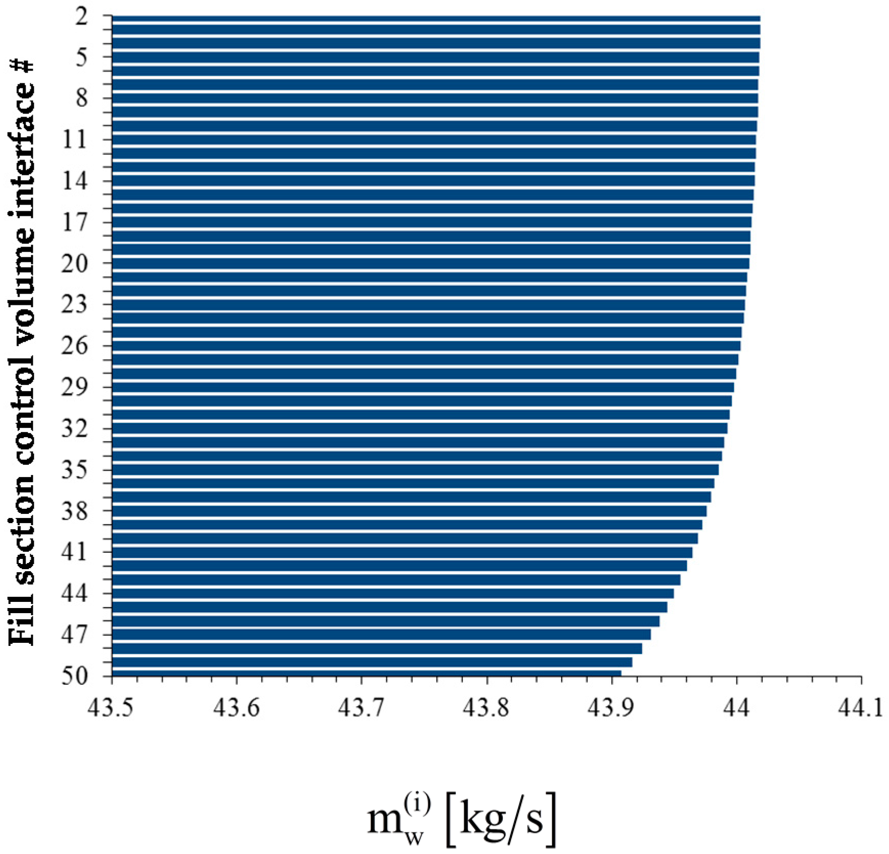
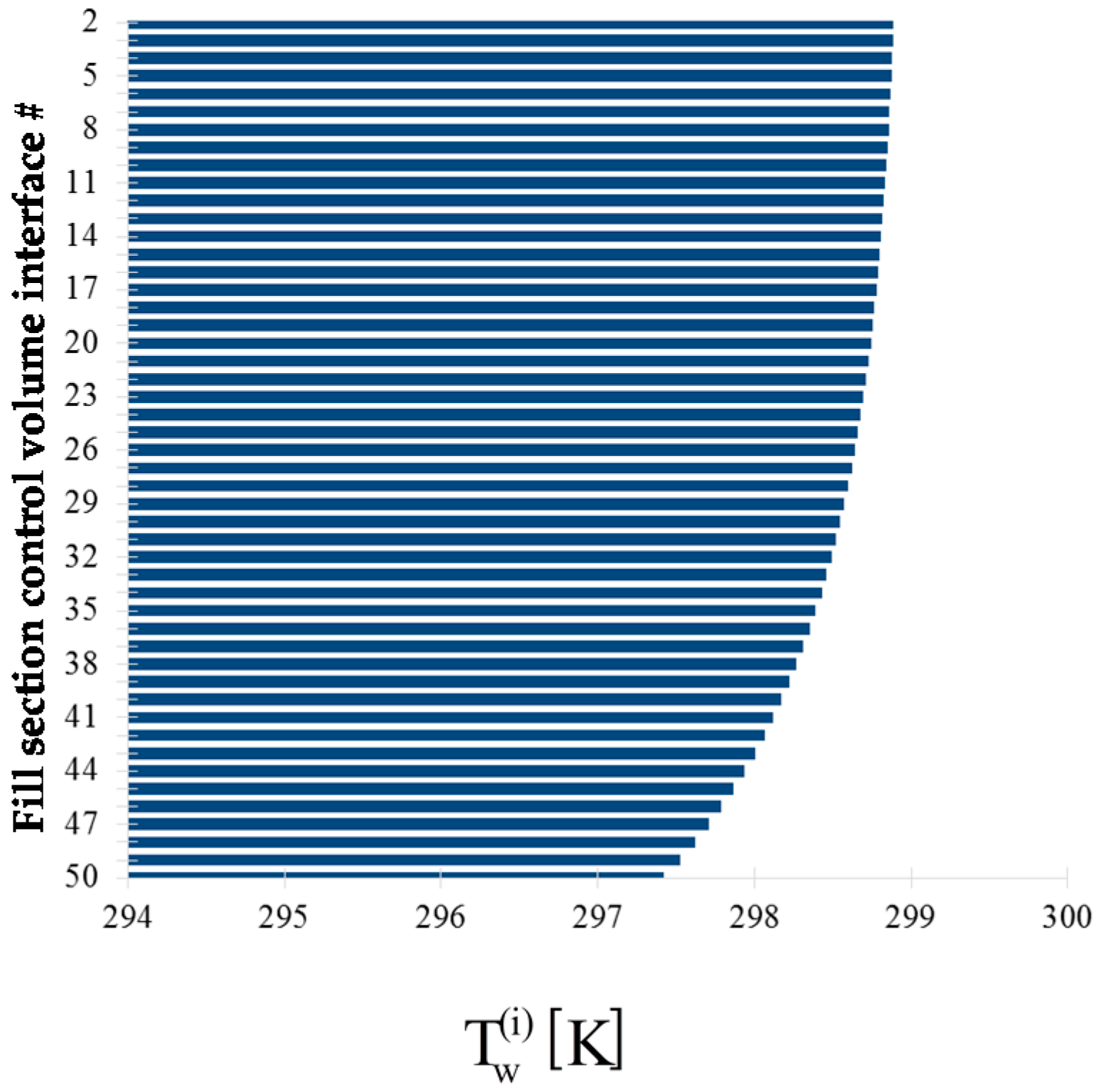
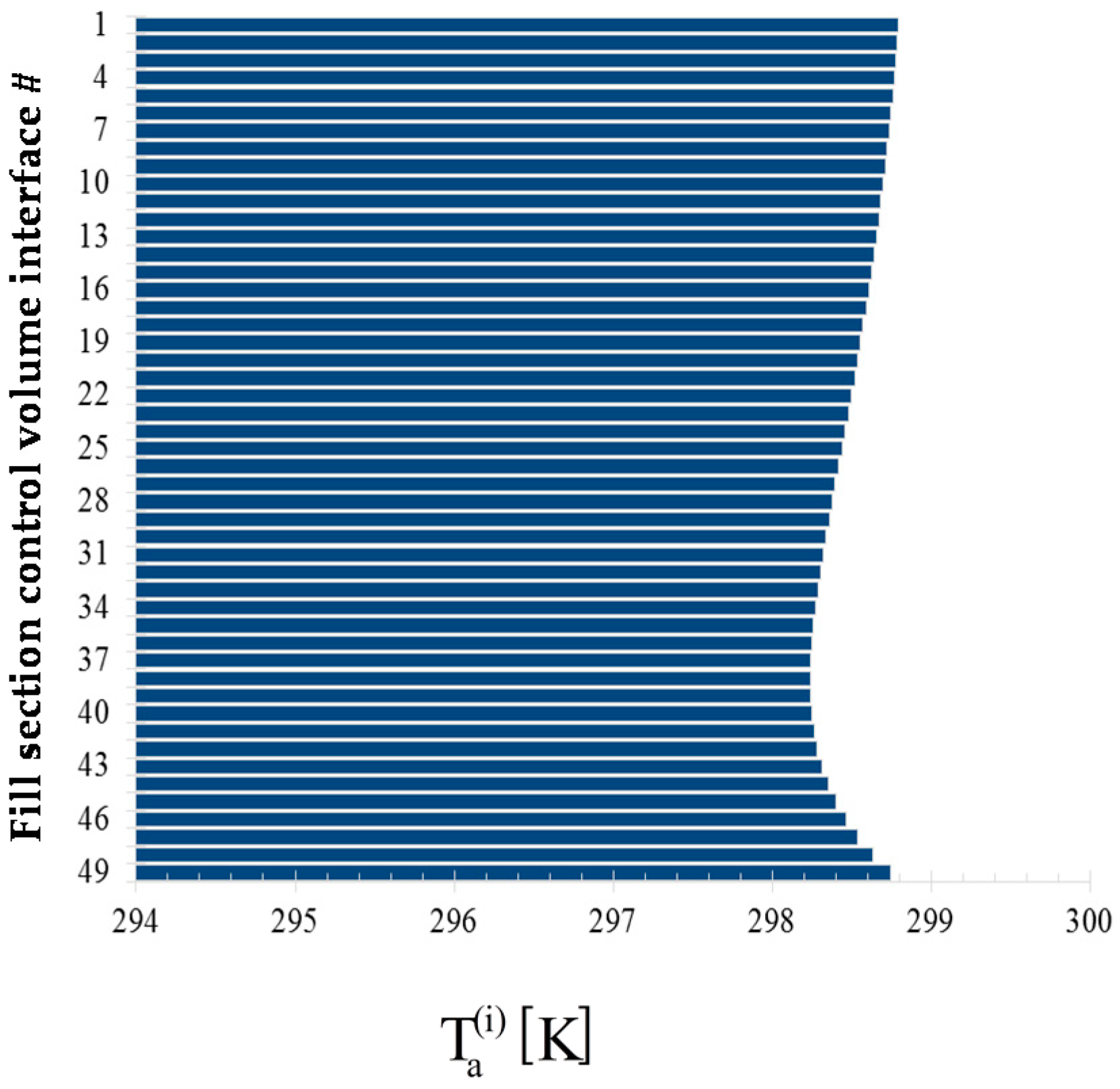
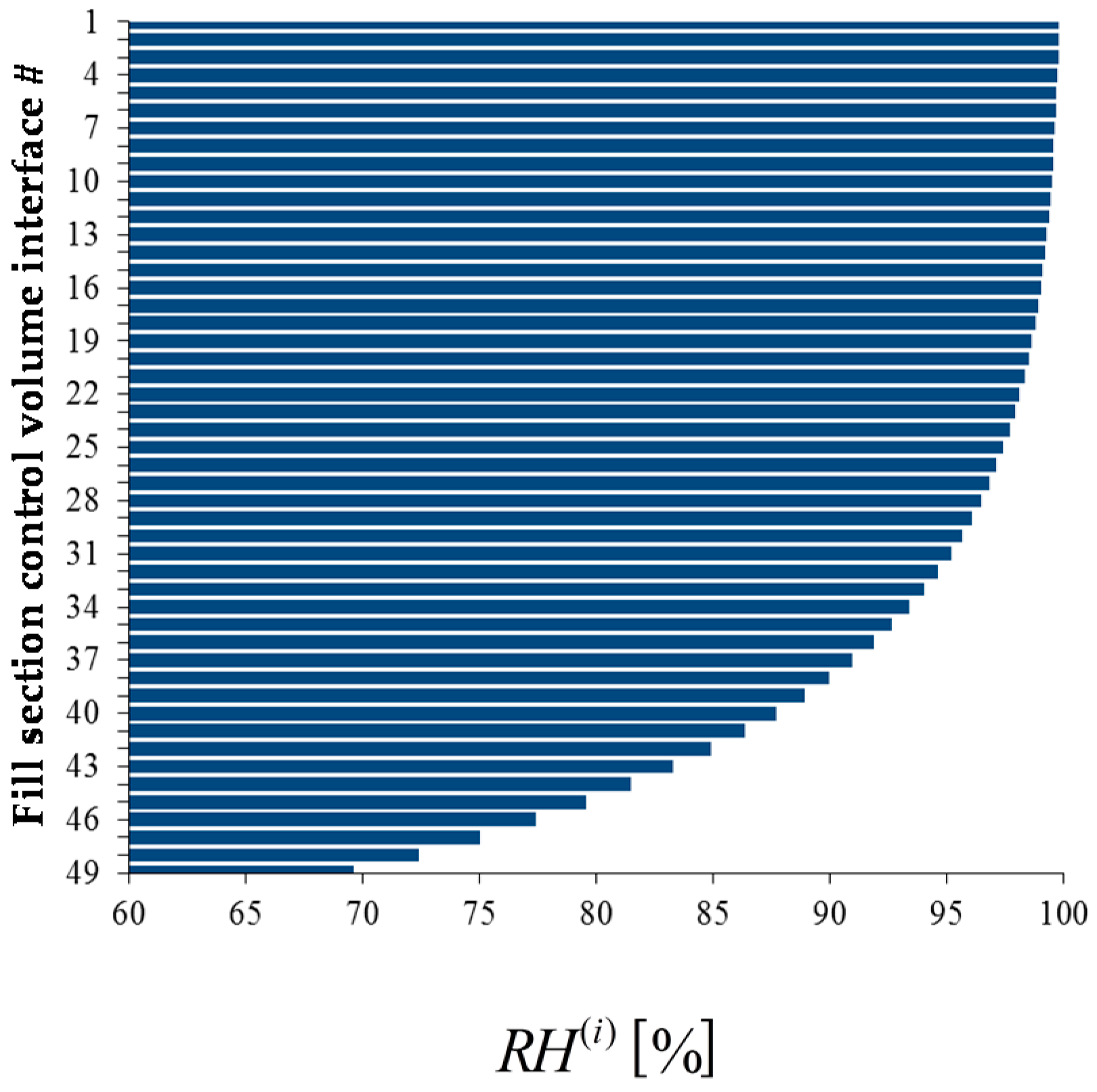
The bar plots displayed below in Figure 4, Figure 5, Figure 6 and Figure 7 show, at the exit of each of the 49 control volumes, the values of the water mass flow rates , the water temperatures , the air temperatures , and the air relative humidity, , respectively.
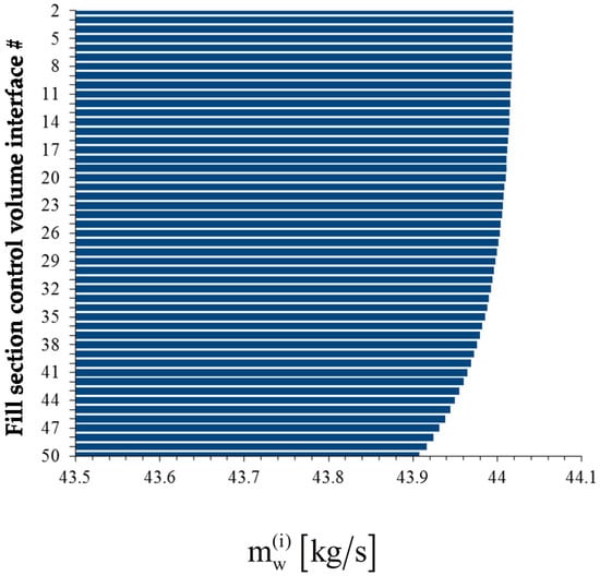
Figure 4.
Bar plot of the water mass flow rates , , at the exit of each control volume along the height of the fill section of the cooling tower.
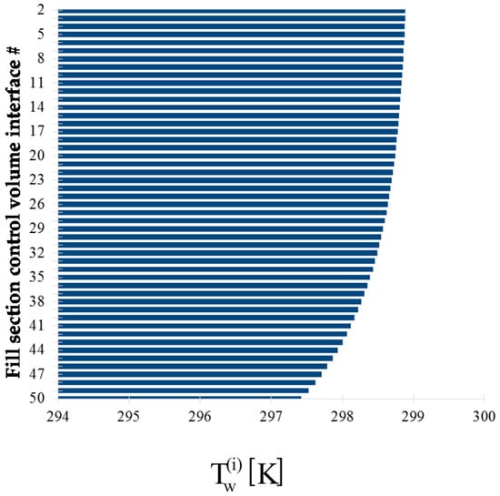
Figure 5.
Bar plot of the outlet water temperature , , at the exit of each control volume along the height of the fill section of the cooling tower.
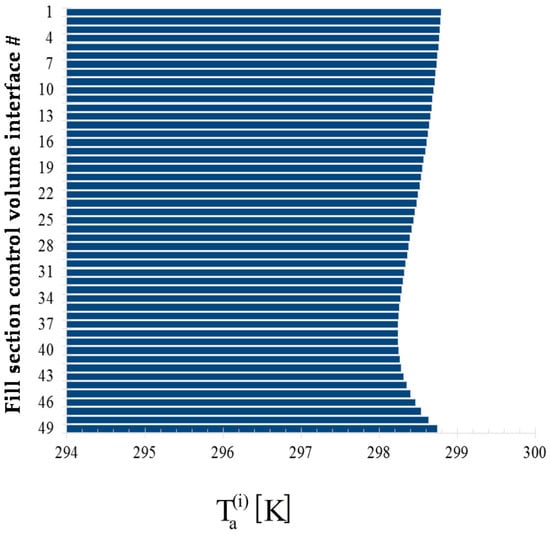
Figure 6.
Bar plot of the outlet air temperature , , at the exit of each control volume along the height of the fill section of the cooling.
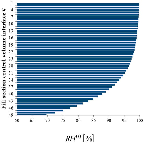
Figure 7.
Bar plot of the outlet air relative humidity , , at the exit of each control volume along the height of the fill section of the cooling.
3. Development of the Cooling Tower Adjoint Sensitivity Model
The development of the cooling tower adjoint sensitivity model follows the same path as in [2], Section 3.1, where the topic is discussed more in detail. The total sensitivity of a model response , with respect to arbitrary variations in the model’s parameters and state functions around the nominal values of the parameters and state functions, is obtained by means of the G-differential of the model’s response to these changes. This G-differential is referred to as , and introducing the adjoint sensitivity functions it becomes:
where the “indirect effect” term, , is obtained as:
and where the vector is required to be the solution of the following adjoint sensitivity system:
The vectors in Equation (20) comprise the functional derivatives of the model responses with respect to the state functions, i.e.,:
and where is defined as follows:
while the vectors in Equation (19) comprise the derivatives of the model’s equations with respect to model parameters, i.e.,:
and where is defined as follows:
It is worth reminding that the adjoint sensitivity system in Equation (20) is independent of parameter variations. This feature allows the selected adjoint functions to be computed by solving the adjoint sensitivity system just once.
Dimensional analysis allows determining the units of the adjoint functions from Equation (19). Namely, the units for the adjoint functions must satisfy the following relations:
where denotes the unit of the response R, while the units for the respective equations are as follows:
Table 1 below lists the units of the adjoint functions for five responses: , , , and , respectively, in which, denotes exit air temperature; denotes exit water temperature; denotes exit air relative humidity; denotes exit water mass flow rate; and denotes air mass flow rate.

Table 1.
Units of the adjoint functions for different responses.
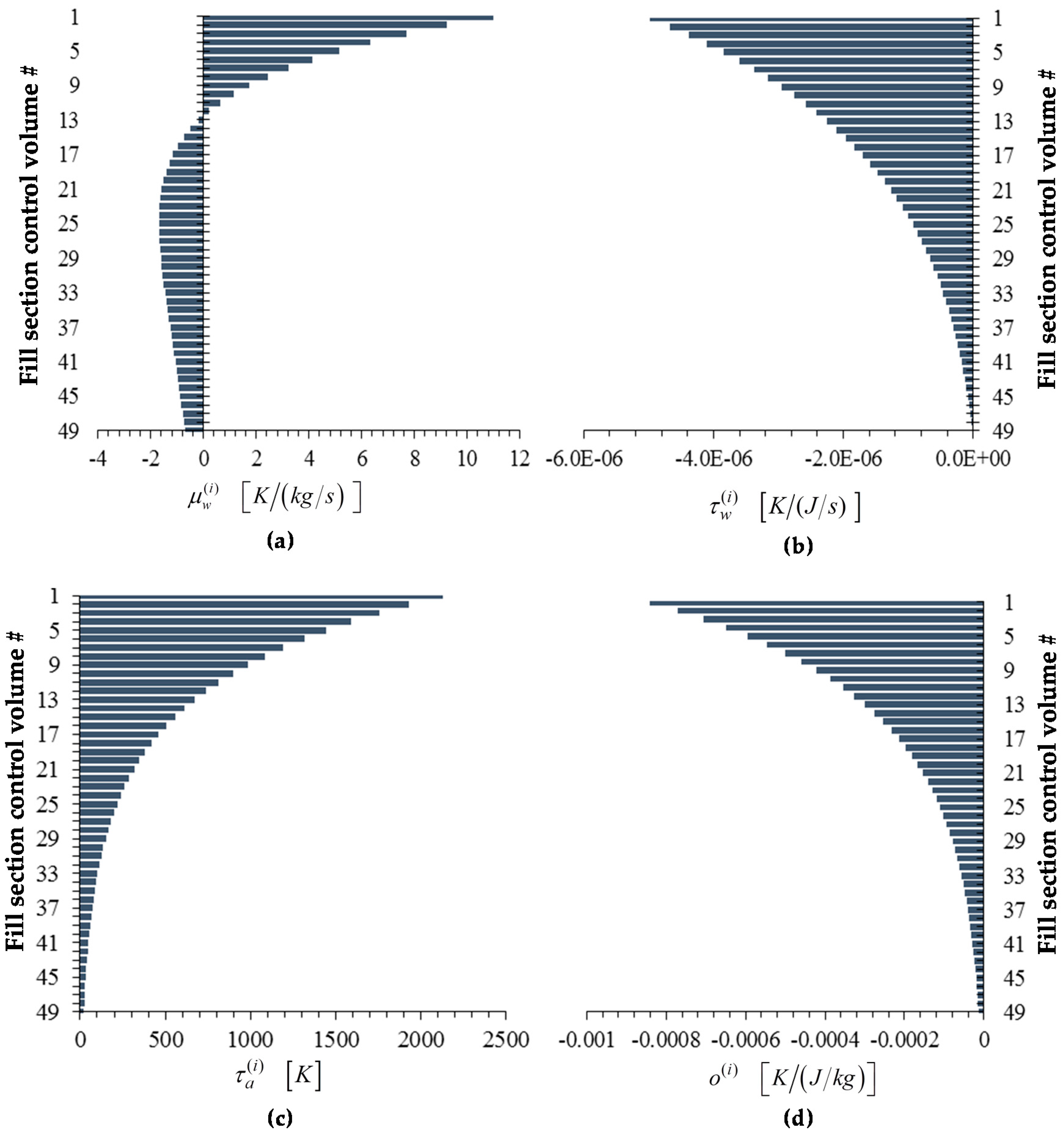
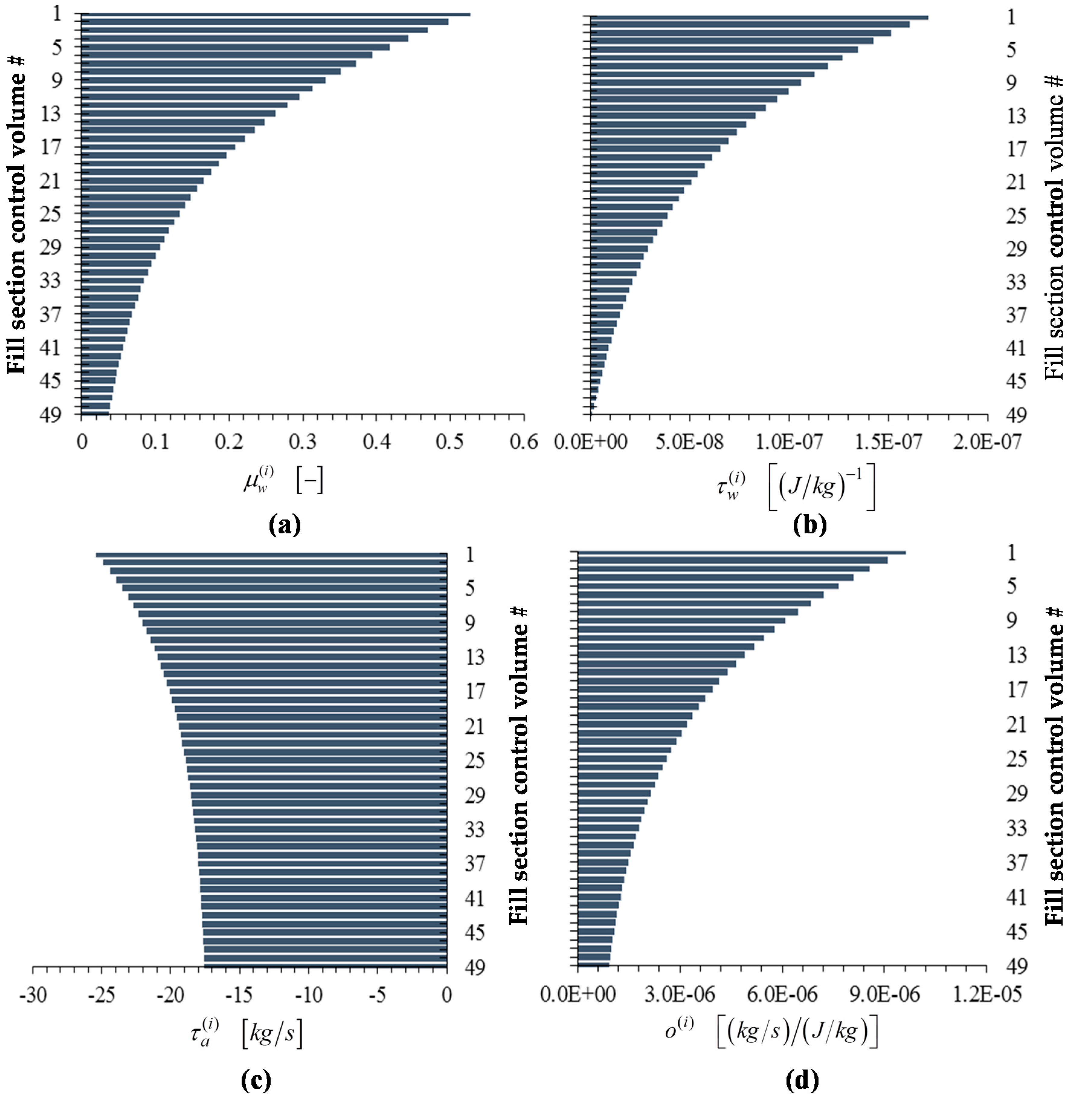
Figure 8, Figure 9, Figure 10, Figure 11 and Figure 12 below display the bar plots of the adjoint functions corresponding to the five measured responses of interest, namely: (i) The exit air temperature ; (ii) The outlet (exit) water temperature ; (iii) The exit air humidity ratio ; (iv) The outlet (exit) water mass flow rate ; and (v) the air mass flow rate .

Figure 8.
Bar plots of adjoint functions for the response as functions of the height of the cooling tower’s fill section: (a) ; (b) ; (c) ; (d) . For the response , the value of the adjoint function is
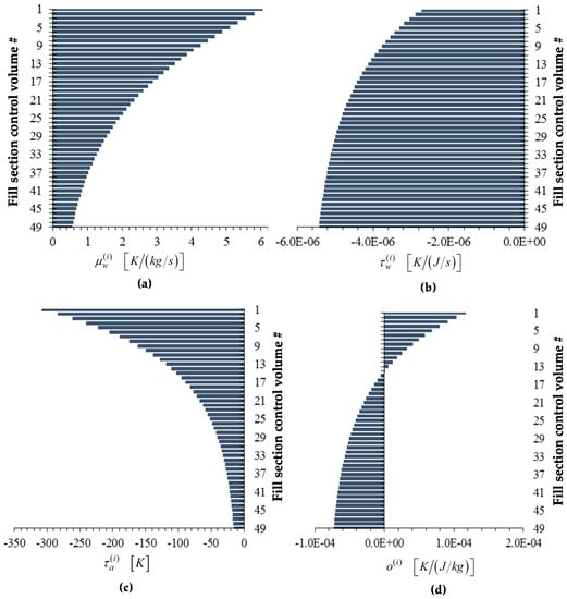
Figure 9.
Bar plots of adjoint functions for the response as functions of the height of the cooling tower’s fill section: (a) ; (b) ; (c) ; (d) . For the response , the value of the adjoint function is
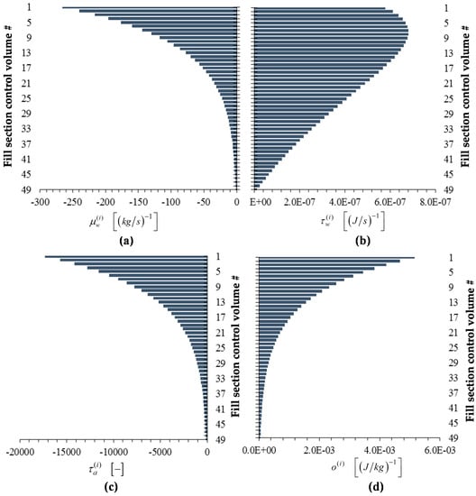
Figure 10.
Bar plots of adjoint functions for the response as functions of the height of the cooling tower’s fill section: (a) ; (b) ; (c) ; (d) . For the response , the value of the adjoint function is
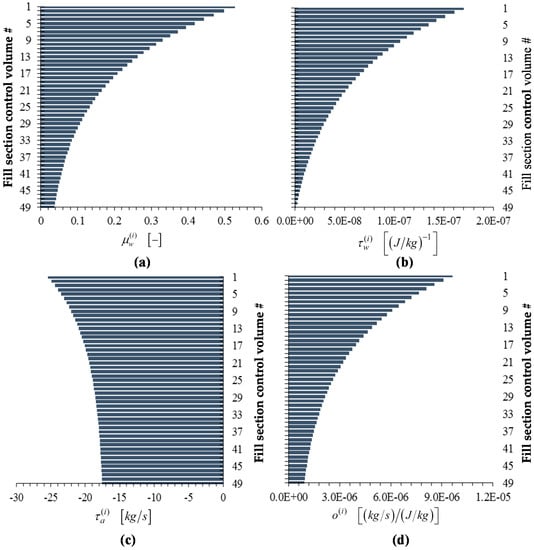
Figure 11.
Bar plots of adjoint functions for the response , as functions of the height of the cooling tower’s fill section: (a) ; (b) ; (c) ; (d) . For the response , the value of the adjoint function is
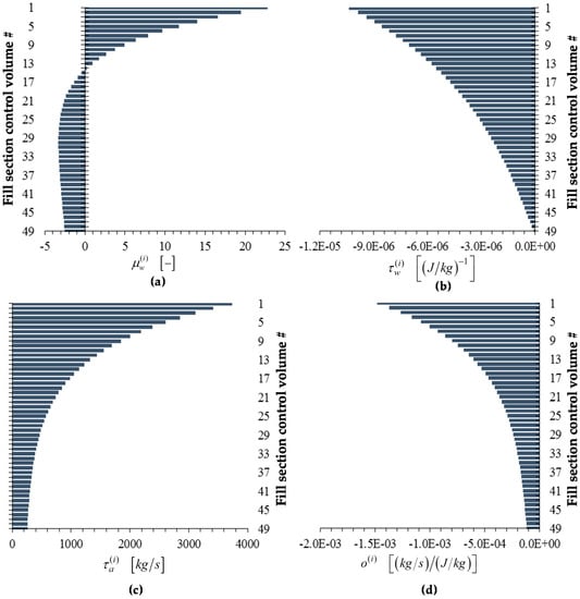
Figure 12.
Bar plots of adjoint functions for the response , as functions of the height of the cooling tower’s fill section: (a) ; (b) ; (c) ; (d) . For the response , the value of the adjoint function is
Let denote the “absolute sensitivity” of the response with respect to the parameter , and is defined as:
An independent method to compute absolute response sensitivities is by making use of perturbative finite difference methods, such as:
- considering an arbitrarily small perturbation to the model parameter ;
- re-computing the perturbed response , where denotes the unperturbed parameter value;
- using the finite difference formula
- using the approximate equality between Equations (27) and (28) to obtain independently the respective values of the adjoint function(s) being verified.
The independent verification methodology discussed in steps (1)–(4) above will be clearly illustrated in Appendix D, where the adjoint functions depicted in Figure 8, Figure 9, Figure 10, Figure 11 and Figure 12 will be verified.
3.1. Sensitivity Analysis Results and Rankings
As has been discussed above, there are a total of 8079 measured benchmark data sets for the cooling tower model operated in “fan-off” regime. As it has also been mentioned, 6717 benchmark data sets (out of the total of 8079 data sets) are considered to correspond to the “unsaturated conditions” which are analyzed in this work. The nominal values for boundary and atmospheric conditions used in this work were obtained from the statistics of these 6717 benchmark data sets corresponding to “unsaturated conditions”. In turn, these “unsaturated” boundary and atmospheric conditions were used to obtain the sensitivity results reported in this Subsection. Section 3.1.1, Section 3.1.2, Section 3.1.3, Section 3.1.4 and Section 3.1.5, below, provide the numerical values and rankings, in descending order, of the relative sensitivities computed using the adjoint sensitivity analysis methodology for the five model responses , , , , and .
Note that the relative sensitivity of a response to a parameter is defined as . Thus, the relative sensitivities are unit-less and are very useful in ranking the parameters to highlight their relative importance for the respective response. Thus, a relative sensitivity of 1.00 indicates that a change of 1% in the respective parameter will induce a 1% change in a response that is linear in the respective sensitivity. The higher the relative sensitivity, the more important the respective parameter to the respective response.
3.1.1. Sensitivity Analysis Results and Rankings for the Outlet Air Temperature,
Table 2 lists the sensitivities, computed using Equations (18) and (19), of the air outlet temperature with respect to all of the model’s parameters. The parameters have been ranked according to the descending order of their relative sensitivities.

Table 2.
Ranked relative sensitivities of the outlet air temperature, .
As the results in Table 2 indicate, the first parameter (i.e., ) has a relative sensitivity around 90%, and is therefore the most important for the air outlet temperature response, , since that means that a 1% change in would induce a 0.91% change in . The next four parameters (i.e., , , , ) have relative sensitivities between 1% and 6%, and are therefore somewhat important. Parameters #6 through #9 (i.e., , , , ) have relative sensitivities between 0.1% and 0.8%. The remaining 38 parameters are relatively unimportant for this response, having relative sensitivities smaller than 1% of the largest relative sensitivity (with respect to ) for this response. Positive sensitivities imply that a positive change in the respective parameter would cause an increase in the response, while negative sensitivities imply that a positive change in the respective parameter would cause a decrease in the response.
3.1.2. Sensitivity Analysis Results and Rankings for the Outlet Water Temperature,
The results and ranking of the relative sensitivities of the outlet water temperature with respect to the most important nine parameters for this response are listed in Table 3. The largest sensitivity of is to the parameter , and has the value of 0.5055; this means that a 1% increase in would induce a 0.5055% increase in . The sensitivities to the remaining 38 model parameters have not been listed since they are smaller than 1% of the largest sensitivity (with respect to ) for this response.

Table 3.
Most important relative sensitivities of the outlet water temperature, .
3.1.3. Sensitivity Analysis Results and Rankings for the Outlet Water Mass Flow Rate,
The results and ranking of the relative sensitivities of the outlet water mass flow rate with respect to the most important 12 parameters for this response are listed in Table 4. This response is most sensitive to (a 1% increase in this parameter would cause a 1.01% increase in the response) and the second largest sensitivity is to the parameter (a 1% increase in this parameter would cause a 0.214% decrease in the response). The sensitivities to the remaining 35 model parameters have not been listed since they are smaller than 1% of the largest sensitivity (with respect to ) for this response.

Table 4.
Most important relative sensitivities of the outlet water mass flow rate, .
3.1.4. Sensitivity Analysis Results and Rankings for the Outlet Air Relative Humidity,
The results and ranking of the relative sensitivities of the outlet air relative humidity with respect to the most important 29 parameters for this response are listed in Table 5. The first three sensitivities of this response are the most relevant; in particular, an increase of 1% in or would cause an increase in the response of 0.27% or 0.25%, respectively. On the other hand, an increase of 1% in would cause a decrease of 0.32% in the response. The sensitivities to the remaining 18 model parameters have not been listed since they are smaller than 1% of the largest sensitivity (with respect to ) for this response.

Table 5.
Most important relative sensitivities of the outlet air relative humidity, .
3.1.5. Relative Sensitivities of the Air Mass Flow Rate,
The results and ranking of the relative sensitivities of the air mass flow rate with respect to the most important 14 parameters for this response are listed in Table 6. The first three sensitivities of this response are very large (relative sensitivities larger than unity are customarily considered to be very significant). In particular, an increase of 1% in or would cause a decrease in the response of 38.51% or 38.49%, respectively. On the other hand, an increase of 1% in would cause an increase of 36% in the response. The sensitivities to the remaining 33 model parameters have not been listed since they are smaller than 1% of the largest sensitivity (with respect to ) for this response.

Table 6.
Most important relative sensitivities of the air mass flow rate, .
Overall, the air mass flow rate, , displays the largest sensitivities, so this response is the most sensitive to parameter variations. The other responses, namely the outlet air temperature, the outlet water temperature, the outlet water mass flow rate and the outlet air relative humidity display sensitivities of comparable magnitude.
3.2. Cross-Comparison of Sensitivity Results
In Table 7, Table 8, Table 9, Table 10 and Table 11, the ranked relative sensitivities for each response are compared side-by-side between three operating conditions, i.e., the two subcases discussed in [2] (partially saturated subcase I, completely saturated subcase II) and the unsaturated case analyzed in this paper. Among the three operating conditions, the “unsaturated case” is defined as a working condition in which air is unsaturated from the inlet to outlet of the cooling tower; while in the saturated subcase II, on the contrary, air is saturated from inlet to outlet of the cooling tower; the saturated subcase I is the combination of the these two cases, i.e., air in the lower portion of the fill section of the cooling tower is in unsaturated conditions, reaching saturation at some point along the height of the tower and remaining saturated in the upper part of the cooling tower. Cross-comparison of sensitivity results reveals the sensitivity variations between the three operating conditions.

Table 7.
Cross-comparison of the top five relative sensitivities for the response of air outlet temperature, .

Table 8.
Cross-comparison of the top five relative sensitivities for the response of water outlet temperature, .

Table 9.
Cross-comparison of the top five relative sensitivities for the response of water outlet mass flow rate, .

Table 10.
Cross-comparison of the top five relative sensitivities for the response of air outlet rel. humidity, .

Table 11.
Cross-comparison of the top five relative sensitivities for the response of air mass flow rate, .
The relative sensitivities and corresponding parameters listed in Table 7 are extracted from Tables 1 and 6 in [3], and Table 2 in this paper. As shown in Table 7, for all three operating conditions, the first most sensitive parameters of the response of air outlet temperature, , is the same (i.e., ). The 2nd and 3rd most sensitive parameter are inverted in the unsaturated case with respect to the two subcases of the saturated case, but with values very close between the two parameters. The parameters that ranks in 4th place for this response is the same for all cases (i.e., ). The 5th parameter is for Subcases I and II and for the unsaturated case.
For the first parameter (i.e., ), the unsaturated case displays the largest sensitivity for this response; subcase II has the smallest sensitivity; while subcase I has an intermediate value of sensitivity between the two. This is expected since subcase I is a mixed case between the unsaturated case and the saturated subcase II, as explained above. For all the remaining parameters in the table the situation is reversed, with Subcase II showing the largest sensitivity values and the unsaturated case presenting the smallest ones, with Subcase I still in the middle. Generally, the sensitivity magnitude of subcase I is slightly closer to that of subcase II. This can be explained by the fact that air remains unsaturated less than half of the height of the fill section, and flows in saturated conditions for more than half of the height of the fill section, as analyzed in [2].
The relative sensitivities and corresponding parameters listed in Table 8 are extracted from Tables 2 and 7 in [3], and Table 3 in this paper. As shown in Table 8, for the response of water outlet temperature, , both the unsaturated case and subcase I are most sensitive to the parameter , whereas subcase II is most sensitive to the parameter . As a comparison, the response of water outlet temperature to the parameter ranks in 3rd place, with a value comparable to the other two cases. The next two most sensitive parameters that rank from 2nd to 3rd places of this response are also different between the operating conditions: for both the unsaturated case and subcase I, parameters and rank in 2nd and 3rd places, respectively; however, for subcase II, parameters that take the 2nd and 3rd places are and , respectively. The parameters that take the 4th and 5th places are also different between the operating conditions, as shown in the table. Overall, for the response of water outlet temperature, , the sensitivity behavior of subcase I is more similar to that of the unsaturated case.
The relative sensitivities and corresponding parameters listed in Table 9 are extracted from Tables 3 and 8 in [3], and Table 4 in this paper. As shown in Table 9, for all three operating conditions, the first two most sensitive parameters of the response of water outlet mass flow rate, , are the same (i.e., and , respectively). In addition, for each of the first two parameters, all three operating conditions have comparable sensitivity magnitudes. This indicates that the sensitivities of the first two parameters are insensitive to the operating condition change. The third most sensitive parameter of this response is different between the operating conditions: for both the unsaturated case and subcase I, this parameter is ; whereas for subcase 2, this parameter is . Similarly, the parameters that take the 4th and 5th places are also different between the operating conditions, as shown in the table.
The relative sensitivities and corresponding parameters listed in Table 10 are extracted from Tables 4 and 9 in [3], and Table 5 in this paper. As shown in Table 10, for Subcases I and II, the first three most sensitive parameters of the response of air outlet relative humidity, , are the same (i.e., , and , respectively); the order is different for the unsaturated case. The next two most sensitive parameters that rank the 4th and 5th places of this response are different between the operating conditions.
For each of the first three parameters, all three operating conditions are sensitive to the parameter changes. In which, subcase II is the most sensitive case; and the unsaturated case is the least sensitive case comparatively. For instance, 1% change in , or will cause around 0.2% change in for the unsaturated case, around 2% change in for subcase I; and nearly 15% change in for subcase II, respectively. Overall, for the response of air outlet relative humidity, , the sensitivity behavior of subcase I is also more similar to that of subcase II, as also the signs of most of the sensitivity values, inverted in the unsaturated case with respect to Subcase I and II, show in Table 10.
The relative sensitivities and corresponding parameters listed in Table 11 are extracted from Tables 5 and 10 in [3], and Table 6 in this paper. As shown in Table 11, for all the operating conditions, the first three most sensitive parameters of the response of air mass flow rate, , are the same (i.e., , and , respectively) with the order of the first two being swapped for the unsaturated case. is the 4th more sensitive parameter in all operating conditions, and with values comparable between the three cases; the parameters ranking in 5th place are different for the three operating conditions.
For each of the first three parameters, all three operating conditions are sensitive to the parameter changes. Differently from the response , subcase II is this time the least sensitive case, while the unsaturated case is the most sensitive case comparatively. For instance, 1% change in , or will cause around 38% change in for the unsaturated case, around 24% change in for subcase I; and nearly 22% change in for subcase II, respectively. Overall, for the response of air mass flow rate, , the sensitivity behavior of subcase I is also more similar to that of subcase II.
3.3. Experimental Data Assimilation, Model Calibration and Best-Estimate Predicted Results with Reduced Predicted Uncertainties
This subsection presents the results of applying the Predictive Modeling of Coupled Multi-Physics Systems (PM_CMPS) methodology [4] to the counter-flow cooling tower model.
The a priori covariance matrix, , of the measured responses (namely: the outlet air temperature, ; the outlet water temperature, , and the outlet air relative humidity, ), cf. Equation (A4), is reproduced below:
The a priori response-parameter covariance matrix, , cf. Equation (A5), is reproduced below:
where the measured correlated parameters are: , and
The a priori parameter covariance matrix, , is:
The a priori covariance matrix of the computed responses, , is given below:
3.3.1. Model Calibration: Predicted Best-Estimated Parameter Values with Reduced Predicted Standard Deviations
The best-estimate nominal parameter values have been computed as follows:
in conjunction with the a priori matrices given in Equations (29)–(32) and the sensitivities presented in Table 1, Table 2, Table 3, Table 4 and Table 5. The resulting best-estimate nominal values are listed in Table 12, below. The corresponding best-estimate absolute standard deviations for these parameters are also presented in this table. These values are the square-roots of the diagonal elements of the matrix . For comparison, the original nominal parameter values and original absolute standard deviations are also listed. As the results in Table 12 indicate, the predicted best-estimate standard deviations are all smaller or at most equal to (i.e., left unaffected) the original standard deviations. The parameters are affected proportionally to the magnitudes of their corresponding sensitivities: the parameters experiencing the largest reductions in their predicted standard deviations are those having the largest sensitivities.

Table 12.
Best-estimated nominal parameter values and their standard deviations.
3.3.2. Predicted Best-Estimated Response Values with Reduced Predicted Standard Deviations
The predicted response covariance matrix, , is as follows:
The non-zero elements with the largest magnitudes of best-estimate response-parameter correlation matrix, , are as follows:
The notation used in Equation (35) is as follows: , ; , .
The resulting best-estimate predicted nominal values are summarized in Table 13. To facilitate comparison, the corresponding measured and computed nominal values are also presented in this table. Note that there are no direct measurements for the outlet water flow rate, . For this response, therefore, the predicted best-estimate nominal value has been obtained by a forward re-computation using the best-estimate nominal parameter values listed in Table 12, while the predicted best estimate standard deviation for this response has been obtained as follows:

Table 13.
Computed, measured, and optimal best-estimate nominal values and standard deviations for the outlet air temperature, outlet water temperature, outlet air relative humidity, outlet water mass flow rate and air mass flow rate responses.
The results presented in Table 13 indicate that the predicted standard deviations are smaller than either the computed or the experimentally measured ones. This is indeed the consequence of using the PM_CMPS methodology in conjunction with consistent (as opposed to discrepant) computational and experimental information. Often, however, the information is inconsistent, usually due to the presence of unrecognized errors. Solutions for addressing such situations have been proposed in [10]. It is also important to note that the PM_CMPS methodology has improved (i.e., reduced, albeit not by a significant amount) the predicted standard deviation for the outlet water flow rate response, for which no measurements were available. This improvement stems from the global characteristics of the PM_CMPS methodology, which combines all of the available simultaneously on phase-space, as opposed to combining it sequentially, as is the case with the current state-of-the-art data assimilation procedures [11,12].
4. Discussion
The original numerical method presented in [1] for the model solution has been replaced in this work with a considerably more accurate and efficient one which guarantees convergence of the computations for all of the available data sets. The adjoint model of the cooling tower has been implemented to compute exactly and efficiently the sensitivities of the model responses to all the 47 model parameters. The adjoint sensitivity model yields the adjoint state functions which are used to compute the sensitivities of each model response to all of the 47 model parameters by means of just one adjoint model computation. These adjoint state functions have been computed and their numerical accuracy has been independently verified. The response sensitivities to all model parameters have been computed for the following responses: (i) the outlet air temperature; (ii) the outlet water temperature; (iii) the outlet water mass flow rate; (iv) the air outlet relative humidity; and (v) air mass flow rate. Thes sensitivities have been subsequently used within the “predictive modeling for coupled multi-physics systems” (PM_CMPS) methodology [4] to obtain: (a) optimal best-estimate prediction for the model parameter values; (b) optimal best-estimate nominal values of the model responses; (c) reduced predicted standard deviations for the best-estimate calibrated model parameter values; and (d) reduced predicted standard deviations for the best-estimate predicted response values.
The results presented in this work show that the PM_CMPS methodology reduces the predicted standard deviation to values that are smaller than both the standard deviations of the measured and the computed response, respectively, even for responses, such as for the air mass flow rate, for which no experimentally measured values are available. This reduction stems from the fact that the PM_CMPS methodology simultaneously combines all the available data in the phase-space; customary data assimilation methodologies [11,12] only allow a sequential combination of the available information. All in all, the application of the PM_CMPS methodology has produced and improved, calibrated and validated model for simulating the functioning of a buoyancy-operated cooling tower under unsaturated conditions. Ongoing work aims at using second-order sensitivities, to be computed by applying the 2nd-ASAM presented in [13,14]. The availability of second-order response sensitivities will enable the computation of non-Gaussian features, such as skewness and kurtosis, of the response distributions of interest.
Acknowledgments
This work has been sponsored by the US Department of Energy under a contract with the University of South Carolina.
Author Contributions
Federico Di Rocco performed all of the numerical calculations in this paper. Dan Gabriel Cacuci conceived and directed the research reported herein, and wrote the paper.
Conflicts of Interest
The authors declare no conflict of interest. The founding sponsors had no role in the design of the study; in the collection, analyses, or interpretation of data; in the writing of the manuscript, and in the decision to publish the results.
Appendix A. Statistical Analysis of Experimentally Measured Responses for SRNL F-Area Cooling Towers
Histogram plots of the 6717 measurement sets considered in this work (each set containing measurements of , , , and ), together with statistical analyses thereof are presented in the remainder of this Appendix.
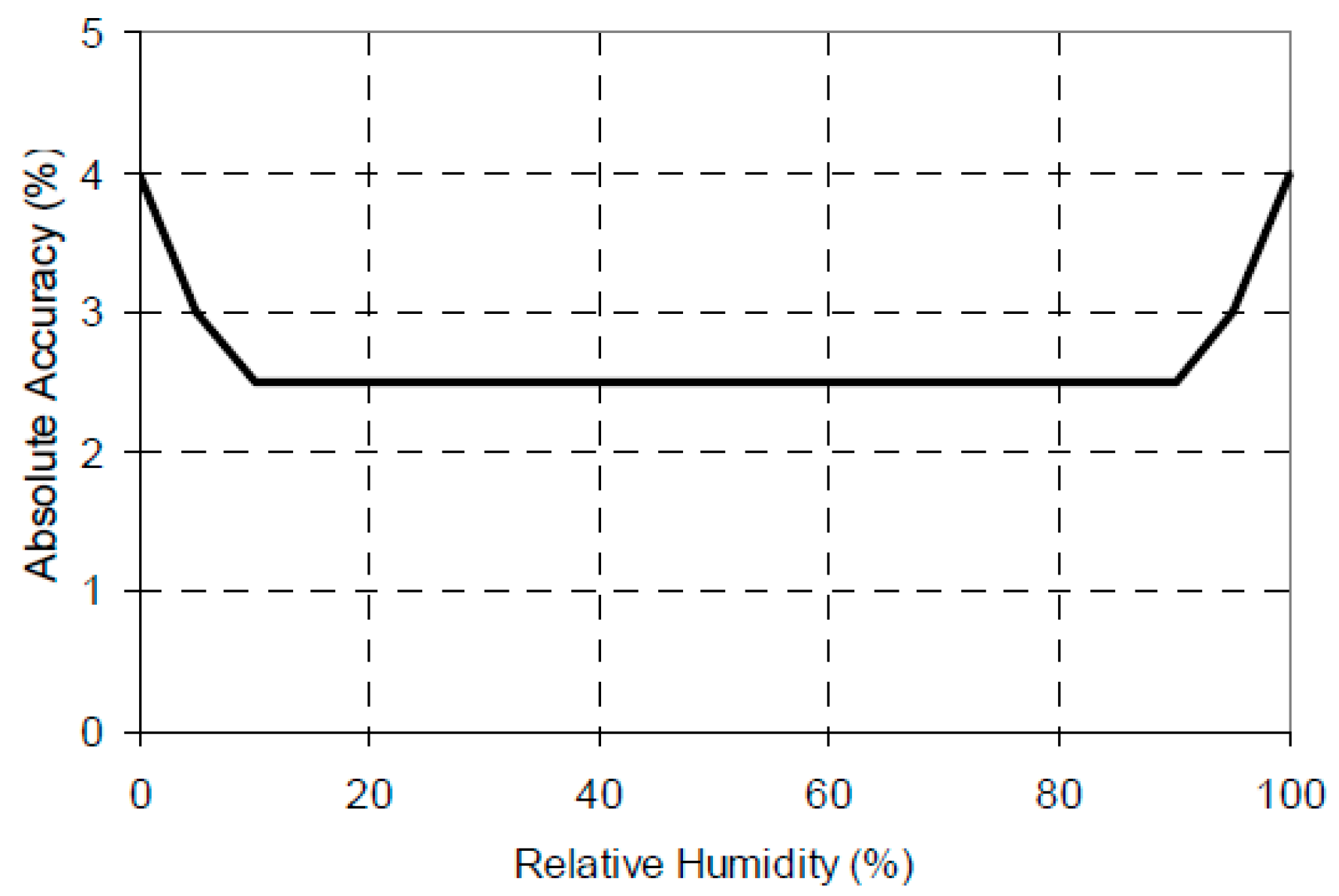
The measured outlet (exit) air relative humidity, , was obtained using Hobo humidity sensors. The accuracy of these sensors is depicted in Figure A1, which indicates the following tolerances (standard deviations): ±2.5% for relative humidity from 10% to 90%; between ±2.5% and ±3.5% for relative humidity from 90% to 95%; and ±3.5%–±4.0% from 95% to 100%. However, when exposed to relative humidity above 95%, the maximum sensor error may temporally increase by an additional 1%, so that the error can reach values between ±4.5% and ±5.0% for relative humidity from 95% to 100%.
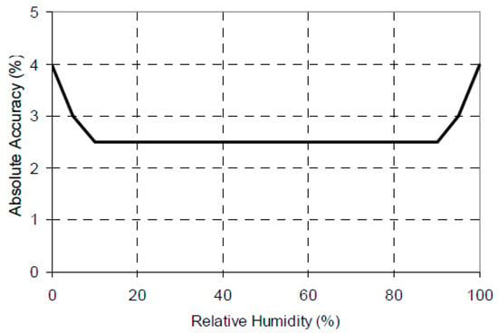
Figure A1.
Humidity sensor accuracy plot (adopted from the specification of HOBO Pro v2).
Figure A1.
Humidity sensor accuracy plot (adopted from the specification of HOBO Pro v2).
As shown in this Figure A2, although the computed relative humidity for each of the 6717 data sets is less than 100%, the measured relative humidity actually spans the range from 33.0% to 104.1%; in this range, 4925 data sets have their respective less than 100% while the other 1792 data sets have their respective over 100%. This situation is nevertheless consistent with the range of the sensors when their tolerances (standard deviations) are taken into account, which would make it possible for a measurement with = 105% to be nevertheless “unsaturated”. Consequently, all the 6717 benchmark data sets plotted in Figure A1, were considered as “unsaturated”, since their respective was less than 105%.
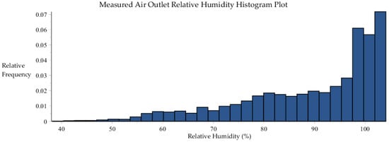
Figure A2.
Histogram plot of the measured air outlet relative humidity, within the 6717 data sets collected by SRNL from F-Area cooling towers.
Figure A2.
Histogram plot of the measured air outlet relative humidity, within the 6717 data sets collected by SRNL from F-Area cooling towers.

The statistical properties of the (measured air outlet relative humidity) distribution shown in Figure A2 have been computed using standard packages, and are presented in Table A1. These statistical properties will be needed for the uncertainty quantification and predictive modeling computations presented in the main body of this work.

Table A1.
Statistics of the air outlet relative humidity distribution [%].
| Minimum | Maximum | Range | Mean | Std. Dev. | Variance | Skewness | Kurtosis |
|---|---|---|---|---|---|---|---|
| 38.2 | 104.1 | 65.9 | 89.61 | 13.63 | 185.72 | −1.01 | 3.22 |
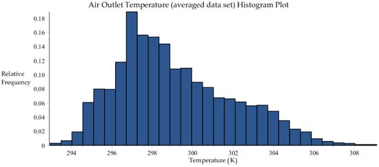
The histogram plots and their corresponding statistical characteristics of the 6717 data sets for the other measurements, namely for: the outlet air temperature [] measured using the “Tidbit” sensors; the outlet air temperature [] measured using the “Hobo” sensors; and the outlet water temperature [] are reported below in Figure A3, Figure A4, Figure A5 and Figure A6, and Table A2, Table A3, Table A4 and Table A5, respectively.
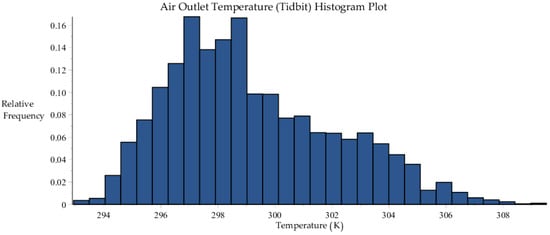
Figure A3.
Histogram plot of the air outlet temperature measured using “Tidbit” sensors, within the 6717 data sets collected by SRNL from F-Area cooling towers.
Figure A3.
Histogram plot of the air outlet temperature measured using “Tidbit” sensors, within the 6717 data sets collected by SRNL from F-Area cooling towers.


Figure A4.
Histogram plot of the air outlet temperature measured using “Hobo” sensors, within the 6717 data sets collected by SRNL from F-Area cooling towers.
Figure A4.
Histogram plot of the air outlet temperature measured using “Hobo” sensors, within the 6717 data sets collected by SRNL from F-Area cooling towers.
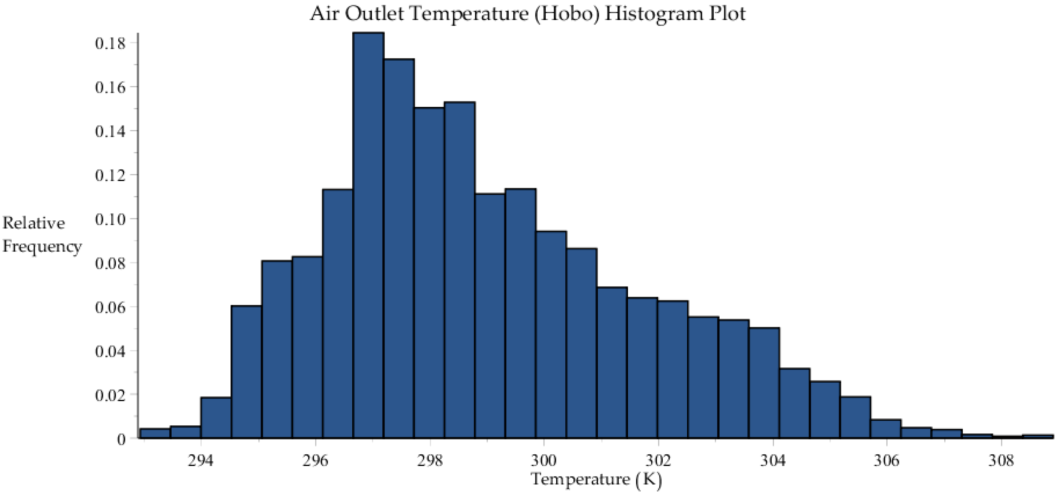

Figure A5.
Histogram plot of water outlet temperature measurements, within the 7688 data sets collected by SRNL from F-Area cooling towers.
Figure A5.
Histogram plot of water outlet temperature measurements, within the 7688 data sets collected by SRNL from F-Area cooling towers.
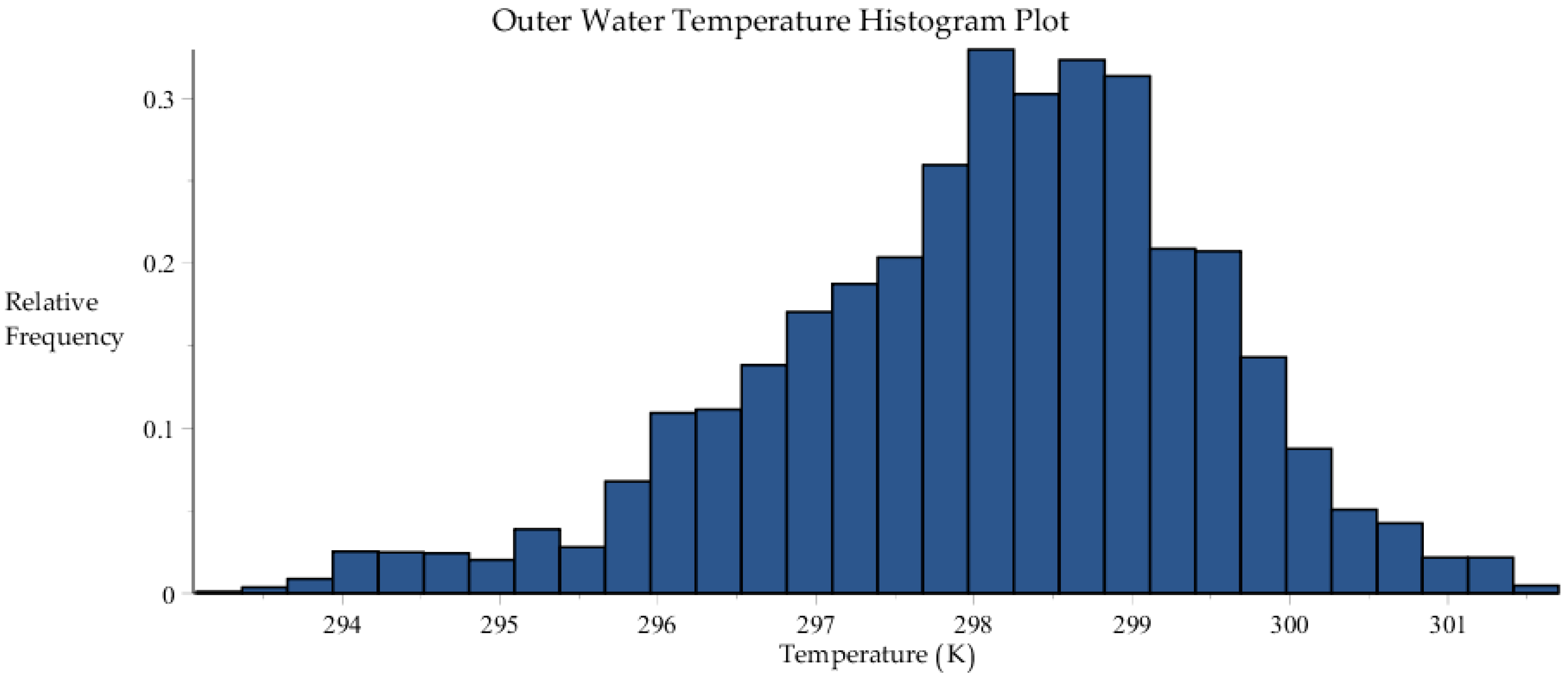

Table A2.
Statistics of the air outlet temperature distribution [K], measured using “Tidbit” sensors.
| Minimum | Maximum | Range | Mean | Std. Dev. | Variance | Skewness | Kurtosis |
|---|---|---|---|---|---|---|---|
| 292.94 | 309.52 | 16.58 | 299.21 | 2.92 | 8.55 | 0.59 | 2.71 |

Table A3.
Air outlet temperature distribution statistics [K], measured using “Hobo” sensors.
| Minimum | Maximum | Range | Mean | Std. Dev. | Variance | Skewness | Kurtosis |
|---|---|---|---|---|---|---|---|
| 292.93 | 308.90 | 15.97 | 299.00 | 2.77 | 7.68 | 0.58 | 2.75 |

Table A4.
Water outlet temperature distribution statistics [K].
| Minimum | Maximum | Range | Mean | Std. Dev. | Variance | Skewness | Kurtosis |
|---|---|---|---|---|---|---|---|
| 293.08 | 301.70 | 8.62 | 298.10 | 1.39 | 1.94 | −0.51 | 3.31 |

Table A5.
Statistics of the averaged air outlet temperature distribution [K].
| Minimum | Maximum | Range | Mean | Std. Dev. | Variance | Skewness | Kurtosis |
|---|---|---|---|---|---|---|---|
| 292.93 | 309.10 | 16.17 | 299.11 | 2.84 | 8.09 | 0.58 | 2.71 |
Ordering the above-mentioned four measured responses as follows: (i) outlet air temperature ; (ii) outlet air temperature ; (iii) outlet water temperature ; and (iv) outlet air relative humidity , yields the following “measured response covariance matrix”, denoted as :
For the purposes of uncertainty quantification, data assimilation, model calibration and predictive modeling, the temperatures measurements provided by the “Tidbit” and “Hobo” sensors can be combined into an “averaged” data set of measured air outlet temperatures, which will be denoted as . The histogram plot and corresponding statistical characteristics of this averaged air outlet temperature are presented in Figure A6 and Table A5, respectively.
Computing the covariance matrix, denoted as , for all of the relevant experimental data for the averaged outlet air temperature , the outlet water temperature , and the outlet air relative humidity , yields the following result:
A comparison between the results in Equations (A1) and (A2) makes clear that the elimination of the second column and row in Equation (A1) yields a 3-by-3 matrix which has entries basically equivalent to the covariance matrix shown in Equation (A2). Therefore, this means that the temperature distributions measured by the “Tidbit” and “Hobo” sensors do not need to be dealt with as separate data sets for the purposes of uncertainty quantification and predictive modeling.
The standard deviation of the humidity sensor utilized for the measurements ( for the response ) have been already considered by including in the category of the “unsaturated” data sets those that have their respective measured relative humidity, , up to 105.0%. In addition to that, the respective uncertainties of the temperature sensors (standard deviations, for both responses and ) must also be taken into consideration for the 6717 data sets. The measuring methods and devices are not dependent with respect to each other, therefore the data standard deviation , stemming from the statistical analysis of the 6717 benchmark data sets, and the sensor standard deviation, , stemming from the instrument’s uncertainty, must stack according to the well-known formula of “addition of the variances of uncorrelated variates”, i.e.,:
Coupling the above relation with the result presented in Equation (A2) will lead to incremented values of the variances on the diagonal of the respective “measured covariance matrix”; this new form of the covariance matrix which will be denoted as . The obtained result is:
In the predictive modeling formalism (which includes uncertainty quantification, data assimilation, and model calibration) the covariance matrix between the measured parameters and responses is required as an input. In the case of interest, all the parameters and responses can be considered as uncorrelated, except for the measured responses considered in this Appendix and the measured parameters listed in Appendix B. The “parameter-response” covariance matrix in Equation (A5), indicated as , refers to the above mentioned parameters (namely: dry-bulb air temperature, ; dew-point air temperature, , inlet water temperature, , atmospheric pressure, , and wind speed ) and responses (i.e., average outlet air temperature, outlet water temperature, and outlet air relative humidity):
Appendix B. Model Parameters for the SRNL F-Area Cooling Towers
The mean values and standard deviations for the independent model parameters presented in Table B1, below, have been derived in collaboration with Dr. Sebastian Aleman of SRNL (private communications, 2016).

Table B1.
Parameters for SRNL F-area cooling towers.
| Index of | Independent Scalar Parameters | C++ String | Math. Notation | Nominal Value(s) | Absolute Std. Dev. | Rel. Std. Dev. (%) |
| 1 | Air temperature (dry bulb) (K) | tdb | 298.882 | 4.034 | 1.35 | |
| 2 | Dew point temperature (K) | tdp | 292.077 | 2.287 | 0.78 | |
| 3 | Inlet water temperature (K) | twin | 298.893 | 1.687 | 0.56 | |
| 4 | Atmospheric pressure (Pa) | patm | 100,588 | 408.26 | 0.41 | |
| 5 | Wind speed (m/s) | wspd | 1.859 | 0.941 | 50.7 | |
| 6 | Sum of loss coefficients above fill | ksum | 10 | 5 | 50 | |
| 7 | Dynamic viscosity of air at T = 300 K (kg/m·s) | muair | 1.983 × 10⁻⁵ | 9.676 × 10⁻⁷ | 4.88 | |
| 8 | Kinematic viscosity of air at T = 300 K (m2/s) | nuair | 1.568 × 10⁻⁵ | 1.895 × 10⁻⁶ | 12.09 | |
| 9 | Thermal conductivity of air at T = 300 K (W/m·K) | tcair | 0.02624 | 1.584 × 10⁻³ | 6.04 | |
| 10 | Heat transfer coefficient multiplier | mlthtc | 1 | 0.5 | 50 | |
| 11 | Mass transfer coefficient multiplier | mltmtc | 1 | 0.5 | 50 | |
| 12 | Fill section frictional loss multiplier | mltfil | 4 | 2 | 50 | |
| 13 | Pvs(T) parameters | a0 | 25.5943 | 0.01 | 0.04 | |
| 14 | a1 | −5229.89 | 4.4 | 0.08 | ||
| 15 | Cpa(T) parameters | A(1) | 1030.5 | 0.2940 | 0.03 | |
| 16 | A(2) | −0.19975 | 0.0020 | 1.00 | ||
| 17 | A(3) | 3.9734 × 10⁻⁴ | 3.345 × 10⁻⁶ | 0.84 | ||
| 18 | Dav(T) parameters | A(1) | 7.06085 × 10⁻⁹ | 0 | 0 | |
| 19 | A(2) | 2.65322 | 0.003 | 0.11 | ||
| 20 | A(3) | −6.1681 × 10⁻³ | 2.3 × 10⁻⁵ | 0.37 | ||
| 21 | A(4) | 6.55266 × 10⁻⁶ | 3.8 × 10⁻⁸ | 0.58 | ||
| 22 | hf(T) parameters | a0f | −1,143,423.78 | 543 | 0.05 | |
| 23 | a1f | 4186.50768 | 1.8 | 0.04 | ||
| 24 | hg(T) parameters | a0g | 2,005,743.99 | 1046 | 0.05 | |
| 25 | a1g | 1815.437 | 3.5 | 0.19 | ||
| 26 | Nu parameters | - | 8.235 | 2.059 | 25 | |
| 27 | - | 0.00314987 | 0.001 | 31.75 | ||
| 28 | - | 0.9902987 | 0.327 | 33.02 | ||
| 29 | - | 0.023 | 0.0088 | 38.26 | ||
| 30 | Cooling tower deck width in x-dir. (m) | dkxw | 8.5 | 0.085 | 1 | |
| 31 | Cooling tower deck width in y-dir. (m) | dkyw | 8.5 | 0.085 | 1 | |
| 32 | Cooling tower deck height above ground (m) | dkht | 10 | 0.1 | 1 | |
| 33 | Fan shroud height (m) | fsht | 3.0 | 0.03 | 1 | |
| 34 | Fan shroud inner diameter (m) | fsid | 4.1 | 0.041 | 1 | |
| 35 | Fill section height (m) | flht | 2.013 | 0.02013 | 1 | |
| 36 | Rain section height (m) | rsht | 1.633 | 0.01633 | 1 | |
| 37 | Basin section height (m) | bsht | 1.168 | 0.01168 | 1 | |
| 38 | Drift eliminator thickness (m) | detk | 0.1524 | 0.001524 | 1 | |
| 39 | Fill section equivalent diameter (m) | deqv | 0.0381 | 0.000381 | 1 | |
| 40 | Fill section flow area (m2) | flfa | 67.29 | 6.729 | 10 | |
| 41 | Fill section surface area (m2) | flsa | 14,221 | 3555.3 | 25 | |
| 42 | Prandlt number of air at T = 80 °C | Pr | 0.708 | 0.005 | 0.71 | |
| 43 | Wetted fraction of fill surface area | wtsa | 1 | 0 | 0 | |
| Index of | Boundary Parameters | C++ String | Math. Notation | Nominal Value | Absolute Std. Dev. | Rel. Std. Dev. (%) |
| 44 | Inlet water mass flowrate (kg/s) | mfwin | 44.0193 | 2.201 | 5 | |
| 45 | Inlet air temperature (K) | tain | set to | 4.034 | 1.35 | |
| 46 | Inlet air humidity ratio (Dependent Scalar Parameter) | hrin | 0.01379 | 0.00192 | 13.80 | |
| Index of | Special Dependent Parameters | C++ String | Math. Notation | Nominal Value | Absolute Std. Dev. | Rel. Std. Dev. (%) |
| 47 | Schmidt number | Sc | 0.5999 | 0.0159 | 2.66 |
The above independent model parameters are used for computing various dependent model parameters and thermal material properties, as shown in Table B2 and Table B3, below.

Table B2.
Dependent scalar model parameters.
| Dependent Scalar Parameters | Math. Notation | Defining Equation or Correlation |
|---|---|---|
| Mass diffusivity of water vapor in air (m2/s) | ||
| Heat transfer coefficient (W/m2·K) | ||
| Mass transfer coefficient (m/s) | ||
| Heat transfer term (W/K) | ||
| Mass transfer term (m3/s) | ||
| Density of dry air (kg/m3) | ||
| Air velocity in the fill section (m/s) | ||
| Fill falling-film surface area per vertical section (m2) | ||
| Rain section inlet flow area (m2) | ||
| Height for natural convection (m) | ||
| Height above fill section (m) | ||
| Fill section control volume height (m) | ||
| Fill section length, including drift eliminator (m) | ||
| Fan shroud inner radius (m) | ||
| Fan shroud flow area (m2) |

Table B3.
Thermal Properties (Dependent Scalar Model Parameters).
| Thermal Properties (Functions of State Variables) | Math. Notation | Defining Equation or Correlation |
|---|---|---|
| hf(Tw) = saturated liquid enthalpy (J/kg) | ||
| Hg(Tw) = saturated vapor enthalpy (J/kg) | ||
| Hg(Ta) = saturated vapor enthalpy (J/kg) | ||
| Cp(T) = specific heat of dry air (J/kg K) | ||
| Pvs(Tw) = saturation pressure (Pa) | ||
| Pvs(Ta) = saturation pressure (Pa) |
Note 1: The measurements of parameters – (i.e., the dry bulb air temperature, dew point temperature, inlet water temperature, atmospheric pressure and wind speed) were taken at the SRNL site, where the F-area cooling towers are located. Out of the 8079 total benchmark data sets [8], 6717 data sets have been considered in this study, since “unsaturated”; through these data sets the statistical properties (means, variance and covariance, skewness and kurtosis) for these model parameters have been derived, as shown in Figure B1, Figure B2, Figure B3, Figure B4 and Figure B5 and Table B4, Table B5, Table B6, Table B7 and Table B8.
Figure B1.
Histogram plot of dry-bulb air temperature data collected by SRNL from F-Area cooling towers.
Figure B1.
Histogram plot of dry-bulb air temperature data collected by SRNL from F-Area cooling towers.
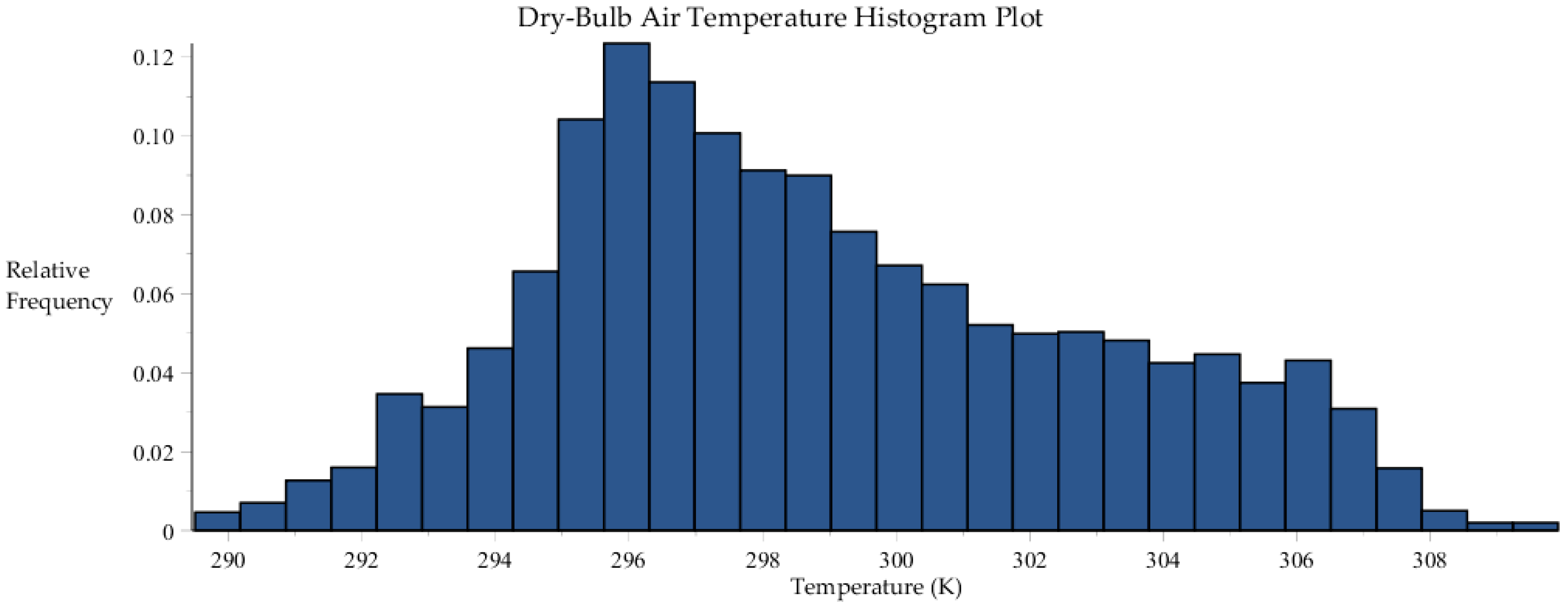

Figure B2.
Histogram plot of dew-point air temperature data collected by SRNL from F-Area cooling towers.
Figure B2.
Histogram plot of dew-point air temperature data collected by SRNL from F-Area cooling towers.
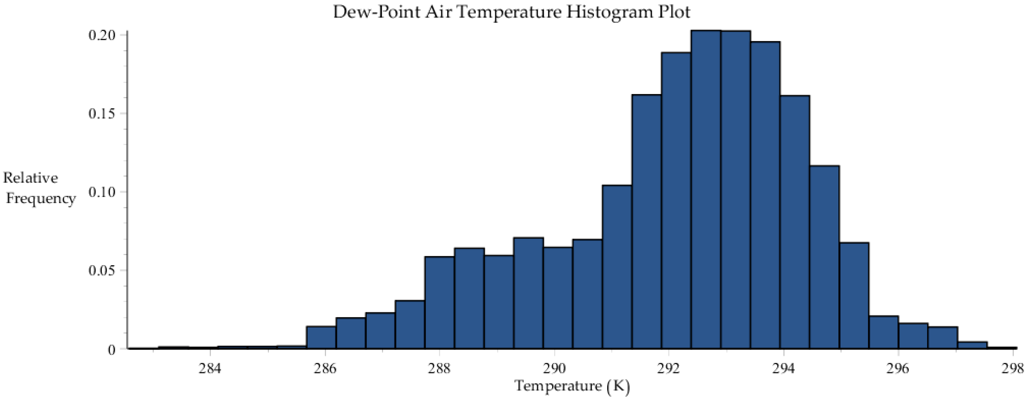
Figure B3.
Histogram plot of inlet water temperature data collected by SRNL from F-Area cooling towers.
Figure B3.
Histogram plot of inlet water temperature data collected by SRNL from F-Area cooling towers.
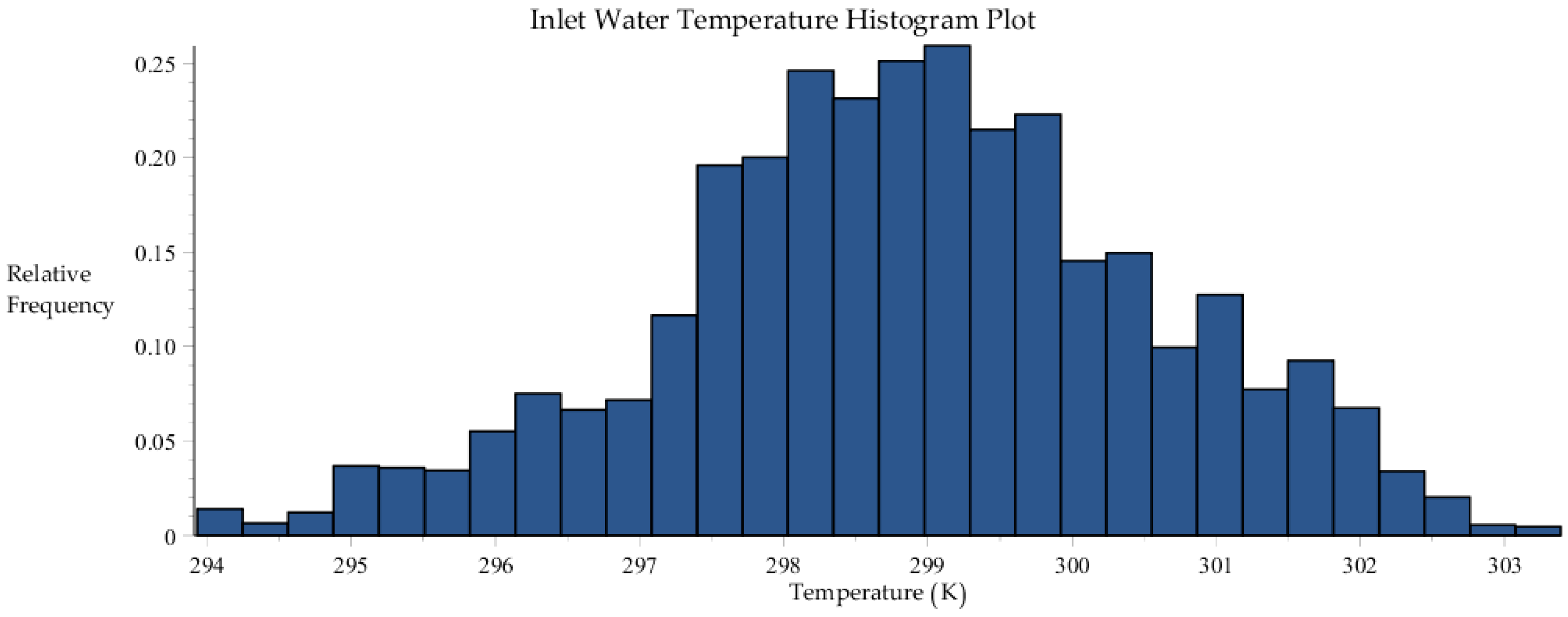
Figure B4.
Histogram plot of atmospheric pressure data collected by SRNL from F-Area cooling towers.
Figure B4.
Histogram plot of atmospheric pressure data collected by SRNL from F-Area cooling towers.

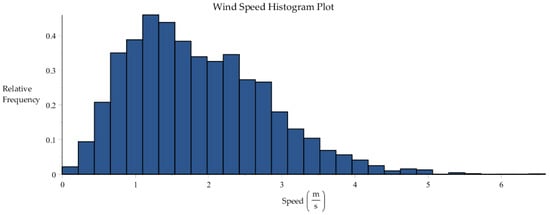
Figure B5.
Histogram plot of wind speed data collected by SRNL from F-Area cooling towers.
Figure B5.
Histogram plot of wind speed data collected by SRNL from F-Area cooling towers.


Table B4.
Statistics of the dry-bulb temperature (set to air inlet temperature) distribution [K].
| Minimum | Maximum | Range | Mean | Std. Dev. | Variance | Skewness | Kurtosis |
|---|---|---|---|---|---|---|---|
| 289.50 | 309.91 | 20.41 | 298.88 | 4.03 | 16.27 | 0.36 | 2.38 |

Table B5.
Statistics of the dew-point temperature distribution [K].
| Minimum | Maximum | Range | Mean | Std. Dev. | Variance | Skewness | Kurtosis |
|---|---|---|---|---|---|---|---|
| 282.58 | 298.06 | 15.48 | 292.08 | 2.29 | 5.23 | −0.66 | 3.11 |

Table B6.
Statistics of the inlet water temperature distribution [K].
| Minimum | Maximum | Range | Mean | Std. Dev. | Variance | Skewness | Kurtosis |
|---|---|---|---|---|---|---|---|
| 293.93 | 303.39 | 9.46 | 298.89 | 1.69 | 2.85 | −0.16 | 2.91 |

Table B7.
Statistics of the atmospheric pressure distribution [Pa].
| Minimum | Maximum | Range | Mean | Std. Dev. | Variance | Skewness | Kurtosis |
|---|---|---|---|---|---|---|---|
| 99617 | 101,677 | 2060 | 100588 | 408.6 | 166,678 | 0.079 | 2.57 |

Table B8.
Statistics of the wind speed distribution [m/s].
| Minimum | Maximum | Range | Mean | Std. Dev. | Variance | Skewness | Kurtosis |
|---|---|---|---|---|---|---|---|
| 0.00 | 6.60 | 6.60 | 1.859 | 0.94 | 0.89 | 0.71 | 3.42 |
The 5-by-5 covariance matrix for the above experimental data has also been computed and is provided below, with the four model parameters ordered as follows: dry-bulb air temperature , dew-point air temperature , inlet water temperature , atmospheric air pressure , and wind speed .
The covariance matrix (above) neglects the uncertainty associated with sensor readings throughout the data collection period. When combining uncertainties by adding variances, the contribution from the sensors is 0.04 K for each of the first three parameters, which accounts for a maximum of ca. 1% of the total variance (for the inlet water temperature, specifically). The uncertainty in the atmospheric pressure sensor is at this time unknown. For these reasons, their contribution to overall uncertainty is considered insignificant at this time.
Appendix C. Derivative Matrix (Jacobian) of the Model Equations with Respect to the State Functions
As mentioned in Section 2, the Jacobian matrix presents similarities with the Jacobian matrix detailed in [2], Equation (C1). More precisely, the sub-matrices whose elements represents the derivatives of Equations (6)–(14) with respect to the vector valued state function remain the same as in [2]; for reasons of brevity, they have not been reported in this paper. On the other side, the sub-matrices whose elements represents the derivatives of Equations (2)–(4) with respect to the vector valued state function , are different from their respective formulations in [2], and therefore they will be hereby detailed with the following notation:
The derivatives of the “liquid continuity equations” (cf., Equations (2)–(4)) with respect to are as follows:
For subsequent use, the above quantities are considered to be the components of the matrix defined as follows:
The derivatives of the “liquid continuity equations” (cf. Equations (2)–(4)) with respect to are as follows:
For subsequent use, the above quantities are considered to be the components of the matrix defined as follows:
The derivatives of the “liquid continuity equations” (cf. Equations (2)–(4)) with respect to are as follows:
For subsequent use, the above quantities are considered to be the components of the matrix defined as follows:
The derivatives of the “liquid continuity equations” (cf. Equations (2)–(4)) with respect to are as follows:
For subsequent use, the above quantities are considered to be the components of the matrix defined as follows:
The derivatives of the “liquid continuity equations” (cf. Equations (2)–(4)) with respect to are as follow follows:
- (1)
- For
- (2)
- For
- (3)
- For
For subsequent use, the above quantities are considered to be the components of the column vector defined as follows:
Appendix D. Derivatives of Cooling Tower Model Equations With Respect to Model Parameters
The differences between the governing equations for this study and for subcase I in [2] concern only the “liquid continuity equations”. Other governing equations (i.e., liquid energy balance equations; water vapor continuity equations; and the air/water vapor energy balance equations) are the same for both cases.
For this reason, the derivatives of Equations (6)–(14) with respect to the model parameters remain the same as in [3], Equation (A3); for reasons of brevity, they have not been reported in this paper. On the other side, the derivatives of Equations (2)–(4) with respect to the model parameters are different from their respective formulations in [3], and therefore they will be hereby detailed with the following notation:
For the sake of brevity, only the nonzero derivatives have been reported in this appendix.
The derivatives of the “liquid continuity equations” (cf. Equations (2)–(4)) with respect to the parameter are as follows:
where:
The derivatives of the “liquid continuity equations” (cf. Equations (2)–(4)) with respect to the parameter are as follows:
The derivatives of the “liquid continuity equations” (cf. Equations (2)–(4)) with respect to the parameter are as follows:
where:
The derivatives of the “liquid continuity equations” (cf. Equations (2)–(4)) with respect to the parameter are as follows:
where:
The derivatives of the “liquid continuity equations” (cf. Equations (A1)–(A4)) with respect to the parameter are as follows:
where:
The derivatives of the “liquid continuity equations” (cf. Equations (2)–(4)) with respect to the parameter are as follows:
where:
The derivatives of the “liquid continuity equations” (cf. Equations (2)–(4)) with respect to the parameter are as follows:
where:
The derivatives of the “liquid continuity equations” (cf. Equations (2)–(4)) with respect to the parameter are as follows:
where was defined previously in Equation (D3), and
The derivatives of the “liquid continuity equations” (cf. Equations (2)–(4)) with respect to the parameter are as follows:
where was defined previously in Equation (D3), and
The derivatives of the “liquid continuity equations” (cf. Equations (2)–(4)) with respect to the parameter are as follows:
where was defined previously in Equation (D3), and
The derivatives of the “liquid continuity equations” (cf. Equations (2)–(4)) with respect to the parameter are as follows:
where was defined previously in Equation (D3), and
The derivatives of the “liquid continuity equations” (cf. Equations (2)–(4)) with respect to the parameter are as follows:
where
The derivatives of the “liquid continuity equations” (cf. Equations (2)–(4)) with respect to the parameter are as follows:
where was defined previously in Equation (D25), and
The derivatives of the “liquid continuity equations” (cf. Equations (2)–(4)) with respect to the parameter are as follows:
where was defined previously in Equation (D25), and
The derivatives of the “liquid continuity equations” (cf. Equations (2)–(4)) with respect to the parameter are as follows:
where was defined previously in Equation (D25), and
The derivatives of the “liquid continuity equations” (cf. Equations (2)–(4)) with respect to the parameter are as follows:
where
The derivatives of the “liquid continuity equations” (cf. Equations (2)–(4)) with respect to the parameter are as follows:
where
The derivatives of the “liquid continuity equations” (cf. Equations (2)–(4)) with respect to the parameter are as follows:
where
The derivatives of the “liquid continuity equations” (cf. Equations (2)–(4)) with respect to the parameter are as follows:
where
The derivatives of the “liquid continuity equations” (cf. Equations (2)–(4)) with respect to the parameter are as follows:
where
The derivatives of the “liquid continuity equations” (cf. Equations (2)–(4)) with respect to the parameter are as follows:
The derivatives of the “liquid continuity equations” (cf. Equations (2)–(4)) with respect to the parameter are as follows:
where
Appendix E. Verification of the Model Adjoint Functions
This appendix provides a complete display of the procedure followed to verify the numerical accuracy of the adjoint functions computed. Five specific adjoint functions have been selected for each of the five responses of the model in such a way that, once those have been verified, all the other adjoint functions would be consequently verified as well. For clarity reasons, the adjoint functions have been grouped based on the response they refer to.
Appendix E.1. Verification of the Adjoint Functions for the Outlet Air Temperature Response
When , the quantities defined in Equations (21)–(22) all vanish except for a single component, namely: Thus, the adjoint functions corresponding to the outlet air temperature response are computed by solving the adjoint sensitivity system given in Equation (20) using as the only non-zero source term; for this case, the solution of Equation (20) has been depicted in Figure 8.
(a) Verification of the adjoint function
Note that the value of the adjoint function obtained by solving the adjoint sensitivity system given in Equation (20) is , as indicated in Figure 8. Now select a variation in the wind speed , and note that Equation (27) yields the following expression for the sensitivity of the response to :
Re-writing Equation (E1) in the form
indicates that the value of the adjoint function could be computed independently if the sensitivity were available, since the quantity is known. To first-order in the parameter perturbation, the finite-difference formula given in Equation (28) can be used to compute the approximate sensitivity ; subsequently, this value can be used in conjunction with Equation (E2) to compute a “finite-difference sensitivity” value, denoted as , for the respective adjoint, which would be accurate up to second-order in the respective parameter perturbation:
Numerically, the wind speed has the nominal (“base-case”) value of . The corresponding nominal value of the response is . Consider next a perturbation , for which the perturbed value of the inlet air temperature becomes . Re-computing the perturbed response by solving Equations (2)–(14) with the value of yields the “perturbed response” value . Using now the nominal and perturbed response values together with the parameter perturbation in the finite-difference expression given in Equation (28) yields the corresponding “finite-difference-computed sensitivity” . Using this value together with the nominal values of the other quantities appearing in the expression on the right side of Equation (E3) yields . This result compares well with the value obtained by solving the adjoint sensitivity system given in Equation (20), cf., below Figure 8.
The same parameter perturbation was utilized to perform the same verification procedure for the adjoint function with respect to the other four responses; Table E1 displays the obtained results, which compare well with the values in the bar plots in Figure 9, Figure 10, Figure 11 and Figure 12.

Table E1.
Verification Table for adjoint function with respect to the responses and
| Response of Interest | ||||||
| Base case | 1.859 | 298.7979 | −0.27219 | −0.12489 | −0.12651 | |
| Perturbed case | 1.84041 | 298.8029 | ||||
| Response of Interest | ||||||
| Base case | 1.859 | 297.4225 | −0.95514 | −0.43824 | −0.43692 | |
| Perturbed case | 1.84041 | 297.4402 | ||||
| Response of Interest | ||||||
| Base case | 1.859 | 99.79724 | −0.71122 | −0.32632 | -0.33332 | |
| Perturbed case | 1.84041 | 99.81046 | ||||
| Response of Interest | ||||||
| Base case | 1.859 | 43.90797 | −0.073996 | −0.033951 | −0.033873 | |
| Perturbed case | 1.84041 | 43.90934 | ||||
| Response of Interest | ||||||
| Base case | 1.859 | 15.83980 | 11.63149 | 5.33677 | 5.34064 | |
| Perturbed case | 1.84041 | 15.62357 | ||||
(b) Verification of the adjoint function
Note that the value of the adjoint function obtained by solving the adjoint sensitivity system given in Equation (20) is , as indicated in Figure 8. Now select a variation in the inlet air temperature , and note that Equation (27) yields the following expression for the sensitivity of the response to :
Re-writing Equation (E4) in the form
indicates that the value of the adjoint function could be computed independently if the sensitivity were available, since the quantities and are known. To first-order in the parameter perturbation, the finite-difference formula given in Equation (28) can be used to compute the approximate sensitivity ; subsequently, this value can be used in conjunction with Equation (E5) to compute a “finite-difference sensitivity” value, denoted as , for the respective adjoint, which would be accurate up to second-order in the respective parameter perturbation:
Numerically, the inlet air temperature has the nominal (“base-case”) value of . The corresponding nominal value of the response is . Consider next a perturbation , for which the perturbed value of the inlet air temperature becomes . Re-computing the perturbed response by solving Equastions (2)–(14) with the value of yields the “perturbed response” value . Using now the nominal and perturbed response values together with the parameter perturbation in the finite-difference expression given in Equation (28) yields the corresponding “finite-difference-computed sensitivity” . Using this value together with the nominal values of the other quantities appearing in the expression on the right side of Equation (E6) yields . This result compares well with the value obtained by solving the adjoint sensitivity system given in Equation (20), cf., Figure 8. When solving this adjoint sensitivity system, the computation of depends on the previously computed adjoint functions ; hence, the forgoing verification of the computational accuracy of also provides an indirect verification that the functions were also computed accurately.
The same parameter perturbation was utilized to perform the same verification procedure for the adjoint function with respect to the other four responses; Table E2 displays the obtained results, which compare well with the values in the bar plots in Figure 9, Figure 10, Figure 11 and Figure 12.

Table E2.
Verification Table for adjoint function with respect to the responses and
| Response of Interest | ||||||
| Base case | 298.882 | 298.7979 | 0.06555 | −1.39 × 10⁻⁵ | −1.31 × 10⁻⁵ | |
| Perturbed case | 298.852 | 298.7960 | ||||
| Response of Interest | ||||||
| Base case | 298.882 | 297.4225 | 0.25125 | −7.21 × 10⁻⁵ | −7.28 × 10⁻⁵ | |
| Perturbed case | 298.852 | 297.4149 | ||||
| Response of Interest | ||||||
| Base case | 298.882 | 99.79724 | 0.09039 | 4.32 × 10⁻⁵ | 5.02 × 10⁻⁵ | |
| Perturbed case | 298.852 | 99.79453 | ||||
| Response of Interest | ||||||
| Base case | 298.882 | 43.90797 | 0.012694 | 9.91 × 10⁻⁷ | 9.18 × 10⁻⁷ | |
| Perturbed case | 298.852 | 43.90758 | ||||
| Response of Interest | ||||||
| Base case | 298.882 | 15.83890 | −2.03711 | −1.22 × 10⁻⁴ | −1.18 × 10⁻⁴ | |
| Perturbed case | 298.852 | 15.90091 | ||||
(c) Verification of the Adjoint Function
Note that the value of the adjoint function obtained by solving the adjoint sensitivity system given in Equation (20) is , as indicated in Figure 8. Now select a variation in the inlet air humidity ratio , and note that Equation (27) yields the following expression for the sensitivity of the response to :
Re-writing Equation (E7) in the form
indicates that the value of the adjoint function could be computed independently if the sensitivity were available, since the has been verified in (the previous) Appendix E.1 (b) and the quantity is known. To first-order in the parameter perturbation, the finite-difference formula given in Equation (28) can be used to compute the approximate sensitivity ; subsequently, this value can be used in conjunction with Equation (E8) to compute a “finite-difference sensitivity” value, denoted as , for the respective adjoint, which would be accurate up to second-order in the respective parameter perturbation:
Numerically, the inlet air humidity ratio has the nominal (“base-case”) value of . The corresponding nominal value of the response is . Consider next a perturbation , for which the perturbed value of the inlet air humidity ratio becomes . Re-computing the perturbed response by solving Eqsuations (2)–(14) with the value of yields the “perturbed response” value . Using now the nominal and perturbed response values together with the parameter perturbation in the finite-difference expression given in Equation (28) yields the corresponding “finite-difference-computed sensitivity” . Using this value together with the nominal values of the other quantities appearing in the expression on the right side of Equation (E9) yields . This result compares well with the value obtained by solving the adjoint sensitivity system given in Equation (20), cf. Figure 8. When solving this adjoint sensitivity system, the computation of depends on the previously computed adjoint functions ; hence, the forgoing verification of the computational accuracy of also provides an indirect verification that the functions were also computed accurately.
The same parameter perturbation was utilized to perform the same verification procedure for the adjoint function with respect to the other four responses; Table E3 displays the obtained results, which compare well with the values in the bar plots in Figure 9, Figure 10, Figure 11 and Figure 12.

Table E3.
Verification Table for adjoint function with respect to the responses and
| Response of Interest | ||||||
| Base case | 0.0137976 | 298.7979 | 11.878 | 21.569 | 21.555 | |
| Perturbed case | 0.0137803 | 298.7977 | ||||
| Response of interest | ||||||
| Base case | 0.0137976 | 297.4225 | 201.180 | −15.593 | −15.799 | |
| Perturbed case | 0.0137803 | 297.4190 | ||||
| Response of interest | ||||||
| Base case | 0.0137976 | 99.79724 | 24.4676 | −152.46 | −152.50 | |
| Perturbed case | 0.0137803 | 99.79681 | ||||
| Response of interest | ||||||
| Base case | 0.0137976 | 43.90797 | 15.1936 | −17.533 | −17.549 | |
| Perturbed case | 0.0137803 | 43.90770 | ||||
| Response of interest | ||||||
| Base case | 0.0137976 | 15.83890 | 43.92139 | 256.109 | 256.059 | |
| Perturbed case | 0.0137803 | 15.83903 | ||||
(d) Verification of the adjoint functions
Note that the values of the adjoint function obtained by solving the adjoint sensitivity system given in Equation (20) is as follows: , as indicated in Figure 8. Now select a variation in the inlet water temperature , and note that Equation (27) yields the following expression for the sensitivity of the response to :
Re-writing Equation (E10) in the form
indicates that the value of the adjoint function could be computed independently if the sensitivity were available, since the quantity is known. To first-order in the parameter perturbation, the finite-difference formula given in Equation (28) can be used to compute the approximate sensitivity ; subsequently, this value can be used in conjunction with Equation (E11) to compute a “finite-difference sensitivity” value, denoted as , for the respective adjoint, which would be accurate up to second-order in the respective parameter perturbation:
Numerically, the inlet water temperature, , has the nominal (“base-case”) value of . As before, the corresponding nominal value of the response is . Consider now a perturbation , for which the perturbed value of the inlet air temperature becomes . Re-computing the perturbed response by solving Equations (2)–(14) with the value of yields the “perturbed response” value . Using now the nominal and perturbed response values together with the parameter perturbation in the finite-difference expression given in Equation (28) yields the corresponding “finite-difference-computed sensitivity” . Using this value together with the nominal values of the other quantities appearing in the expression on the right side of Equation (E12) yields . This result compares well with the value obtained by solving the adjoint sensitivity system given in Equation (20), cf. Figure 8.
The same parameter perturbation was utilized to perform the same verification procedure for the adjoint function with respect to the other four responses; Table E4 displays the obtained results, which compare well with the values in the bar plots in Figure 9, Figure 10, Figure 11 and Figure 12.

Table E4.
Verification Table for adjoint function with respect to the responses and
| Response of Interest | ||||||
| Base case | 298.893 | 298.7979 | 0.91889 | −4.99 × 10⁻⁶ | −4.98 × 10⁻⁶ | |
| Perturbed case | 298.873 | 298.7795 | ||||
| Response of interest | ||||||
| Base case | 298.893 | 297.4225 | 0.50358 | −2.73 × 10⁻⁶ | −2.73 × 10⁻⁶ | |
| Perturbed case | 298.873 | 297.4124 | ||||
| Response of interest | ||||||
| Base case | 298.893 | 99.79724 | −0.10693 | 5.77 × 10⁻⁷ | 5.78 × 10⁻⁷ | |
| Perturbed case | 298.873 | 99.7994 | ||||
| Response of interest | ||||||
| Base case | 298.893 | 43.90797 | −0.031364 | 1.70 × 10⁻⁷ | 1.70 × 10⁻⁷ | |
| Perturbed case | 298.873 | 43.90859 | ||||
| Response of interest | ||||||
| Base case | 298.893 | 15.83980 | 1.91042 | −1.037 × 10⁻⁵ | −1.035 × 10⁻⁵ | |
| Perturbed case | 298.873 | 15.80159 | ||||
(e) Verification of the adjoint function
Note that the values of the adjoint function obtained by solving the adjoint sensitivity system given in Equation (20) is as follows: , as indicated in Figure 8. Now select a variation in the inlet water mass flow rate , and note that Equation (27) yields the following expression for the sensitivity of the response to :
Since the adjoint functions and have been already verified as described in Appendix E.1 (b) and Appendix E.1 (c), it follows that the computed values of adjoint functions can also be considered as being accurate, since they constitute the starting point for solving the adjoint sensitivity system in Equation (20); was proved being accurate in Appendix E.1 (d).
Re-writing Equation (E13) in the form
indicates that the value of the adjoint function could be computed independently if the sensitivity were available, since all the other quantities are known. To first-order in the parameter perturbation, the finite-difference formula given in Equation (28) can be used to compute the approximate sensitivity ; subsequently, this value can be used in conjunction with Equation (E14) to compute a “finite-difference sensitivity” value, denoted as , for the respective adjoint, which would be accurate up to second-order in the respective parameter perturbation:
Numerically, the inlet water mass flow rate, , has the nominal (“base-case”) value of . As before, the corresponding nominal value of the response is . Consider now a perturbation , for which the perturbed value of the inlet air temperature becomes . Re-computing the perturbed response by solving Equations (2)–(14) with the value of yields the “perturbed response” value . Using now the nominal and perturbed response values together with the parameter perturbation in the finite-difference expression given in Equation (28) yields the corresponding “finite-difference-computed sensitivity” . Using this value together with the nominal values of the other quantities appearing in the expression on the right side of Equation (E15) yields . This result compares well with the value obtained by solving the adjoint sensitivity system given in Equation (20), cf. Figure 8.
The same parameter perturbation was utilized to perform the same verification procedure for the adjoint function with respect to the other four responses; Table E5 displays the obtained results, which compare well with the values in the bar plots in Figure 9, Figure 10, Figure 11 and Figure 12.

Table E5.
Verification Table for adjoint function with respect to the responses and
| Response of Interest | ||||||
| Base case | 44.0193 | 298.7979 | 0.00328 | 10.977 | 10.301 | |
| Perturbed case | 43.9893 | 298.7978 | ||||
| Response of Interest | ||||||
| Base case | 44.0193 | 297.4225 | 0.03142 | 6.0444 | 6.0443 | |
| Perturbed case | 43.9893 | 297.4215 | ||||
| Response of Interest | ||||||
| Base case | 44.0193 | 99.79724 | −0.001267 | −265.511 | −265.511 | |
| Perturbed case | 43.9893 | 99.79728 | ||||
| Response of interest | ||||||
| Base case | 44.0193 | 43.90797 | 0.99986 | 0.52753 | 0.52753 | |
| Perturbed case | 43.9893 | 43.87797 | ||||
| Response of Interest | ||||||
| Base case | 44.0193 | 15.83980 | 0.010543 | 22.807 | 22.807 | |
| Perturbed case | 43.9893 | 15.83948 | ||||
References
- Aleman, S.E.; Garrett, A.J. Operational Cooling Tower Model (CTTool v1.0); SRNL-STI-2015-00039, Revision 0; Savannah River National Laboratory: Savannah River Site, SC, USA, 2015. [Google Scholar]
- Cacuci, D.G.; Di Rocco, F. Predictive modeling of a buoyancy-operated cooling tower operating under saturated Conditions. I: Adjoint sensitivity model. Nucl. Sci. Eng. 2016, in press. [Google Scholar]
- Di Rocco, F.; Cacuci, D.G.; Badea, M.C. Predictive modeling of a buoyancy-operated cooling tower operating under saturated Conditions. II: Optimal best-estimate results with reduced predicted uncertainties. Nucl. Sci. Eng. 2016, in press. [Google Scholar]
- Cacuci, D.G. Sensitivity theory for nonlinear systems: I. Nonlinear functional analysis approach. J. Math. Phys. 1981, 22, 2794–2802. [Google Scholar] [CrossRef]
- Cacuci, D.G. Sensitivity and Uncertainty Analysis: Theory; Chapman & Hall/CRC: Boca Raton, FL, USA, 2003. [Google Scholar]
- Cacuci, D.G.; Ionescu-Bujor, M.; Navon, I.M. Sensitivity and Uncertainty Analysis: Applications to Large Scale Systems; Chapman & Hall/CRC: Boca Raton, FL, USA, 2005. [Google Scholar]
- Cacuci, D.G. Predictive modeling of coupled multi-physics systems: I. theory. Ann. Nucl. Energy 2014, 70, 266–278. [Google Scholar] [CrossRef]
- Garrett, A.J.; Parker, M.J.; Villa-Aleman, E. 2004 Savannah River site Cooling Tower Collection; SRNL-DOD-2005-07; Atmospheric Technologies Group, Savannah River National Laboratory: Aiken, SC, USA, 2005. [Google Scholar]
- Saad, Y.; Schultz, M.H. GMRES: A generalized minimal residual algorithm for solving nonsymmetric linear systems. SIAM J. Sci. Stat. Comput. 1986, 7, 856–869. [Google Scholar] [CrossRef]
- Oppe, T.C.; Joubert, W.D.; Kincaid, D.R. A Package for Solving Large Sparse Linear Systems by Various Iterative Methods; NSPCG User’s Guide, Version 1.0; Center for Numerical Analysis, the University of Texas at Austin: Austin, TX, USA, 1988. [Google Scholar]
- Faragó, I.; Havasi, A.; Zlatev, Z. Advanced Numerical Methods for Complex Environmental Models: Needs and Availability; Bentham Science Publishers: Oak Park, IL, USA, 2014. [Google Scholar]
- Cacuci, D.G.; Navon, I.M.; Ionescu-Bujor, M. Computational Methods for Data Evaluation and Assimilation; Chapman & Hall/CRC: Boca Raton, FL, USA, 2014. [Google Scholar]
- Cacuci, D.G. Second-order adjoint sensitivity analysis methodology (2nd-ASAM) for large-scale nonlinear Systems: I. Theory. Nucl. Sci. Eng. 2016, 184, 16–30. [Google Scholar]
- Cacuci, D.G. Second-Order adjoint sensitivity analysis methodology (2nd-ASAM) for large-scale nonlinear Systems: II. Illustrative application to a paradigm nonlinear heat conduction benchmark. Nucl. Sci. Eng. 2016, 184, 31–52. [Google Scholar] [CrossRef]
© 2016 by the authors; licensee MDPI, Basel, Switzerland. This article is an open access article distributed under the terms and conditions of the Creative Commons Attribution (CC-BY) license (http://creativecommons.org/licenses/by/4.0/).

