2.2. The Stochastic Model
The crude oil spot price denoted by
S can be assumed to evolve stochastically in accordance with a mean-reverting process (MR) as per Equation (1):
In this equation
is the long-term equilibrium value towards which the spot price
tends to revert in the long-term,
k is the speed of reversion that determines how the expected value of
approximates in time to the long-term equilibrium value
,
σ is the volatility and
is the increment of a Wiener process with
. Let
λ be the market price of risk, then the behavior in the risk-neutral word (this is the futures market case) is:
Abadie and Chamorro (2013) [
18] show that in the risk-neutral world the expected value under the equivalent martingale measure or risk-neutral measure in the moment
t for the future price with maturity
T is:
A similar Equation (4) can be used with the future with the nearest maturity denoted by
T1 to estimate the future price with maturity
T2:
Equation (4) enables estimates for each day to be drawn up for the values and .
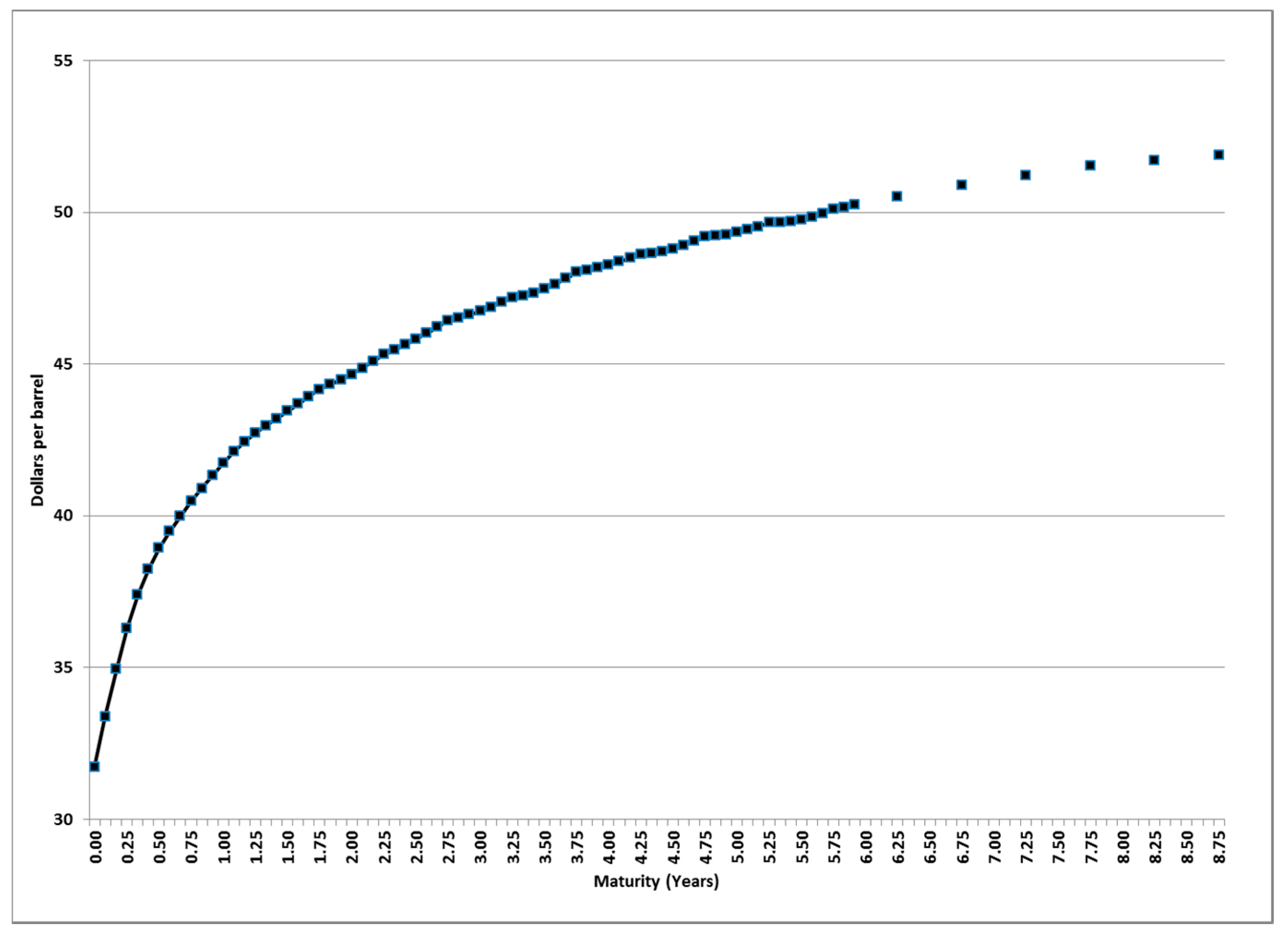
In the long-term there is a long-term equilibrium value given by Equation (5):
Initially we calculate
k + λ and
S* for each day using nonlinear least squares, which results in 2571 values of each parameter. More information about the parameters calculation can be found in
Appendix A. We obtain the time-series
, but there are some outliers, so we refine it using the procedure described in
Appendix B.
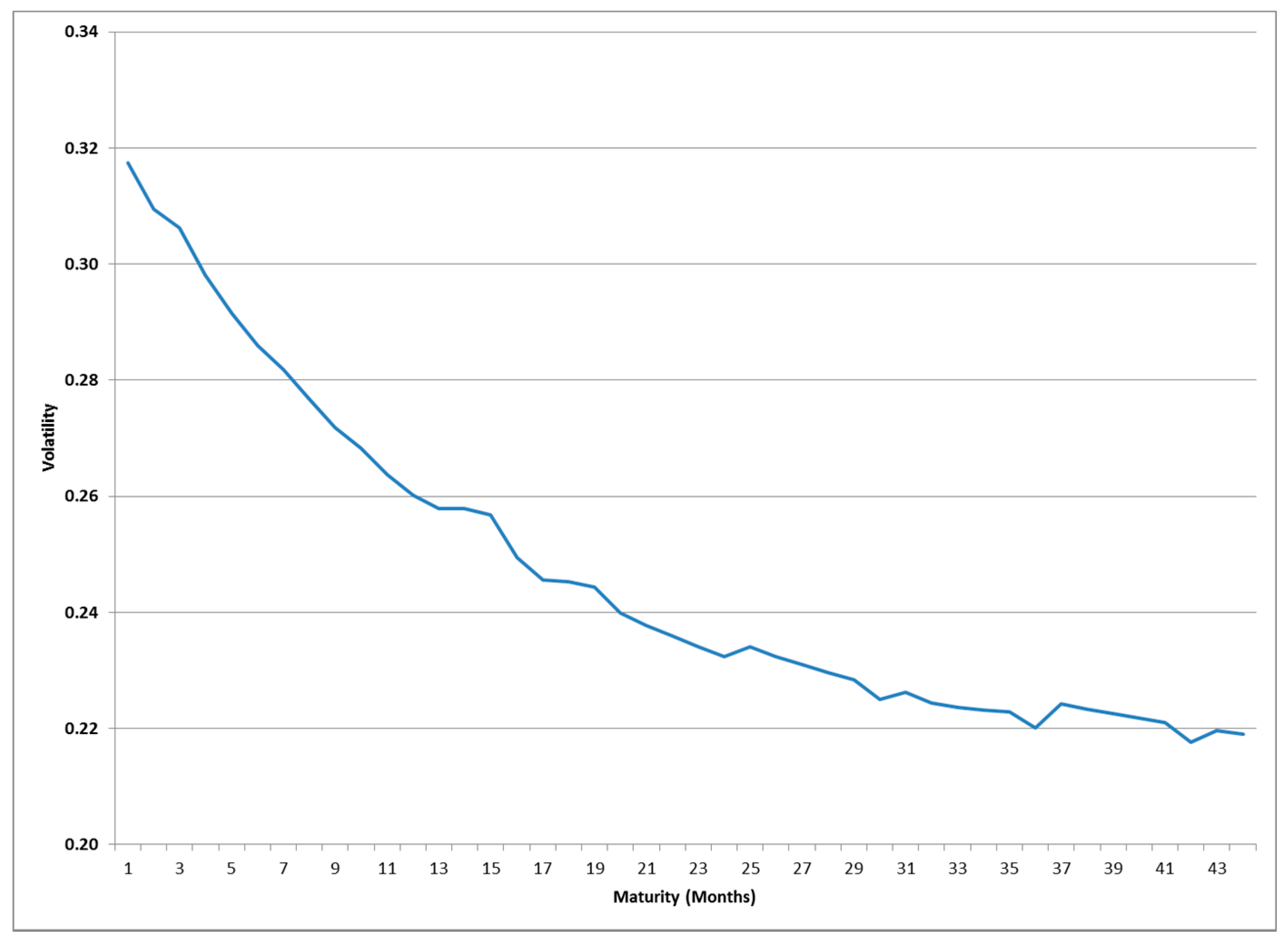
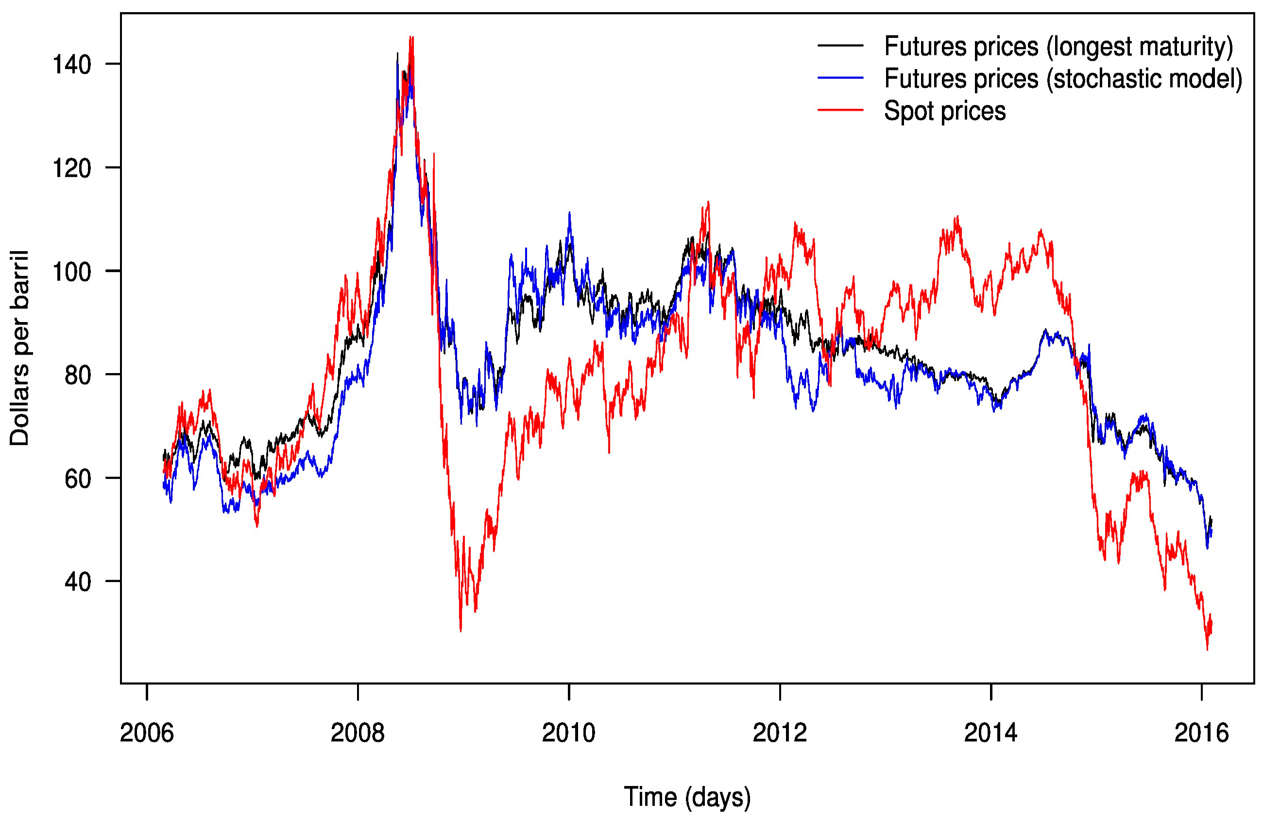
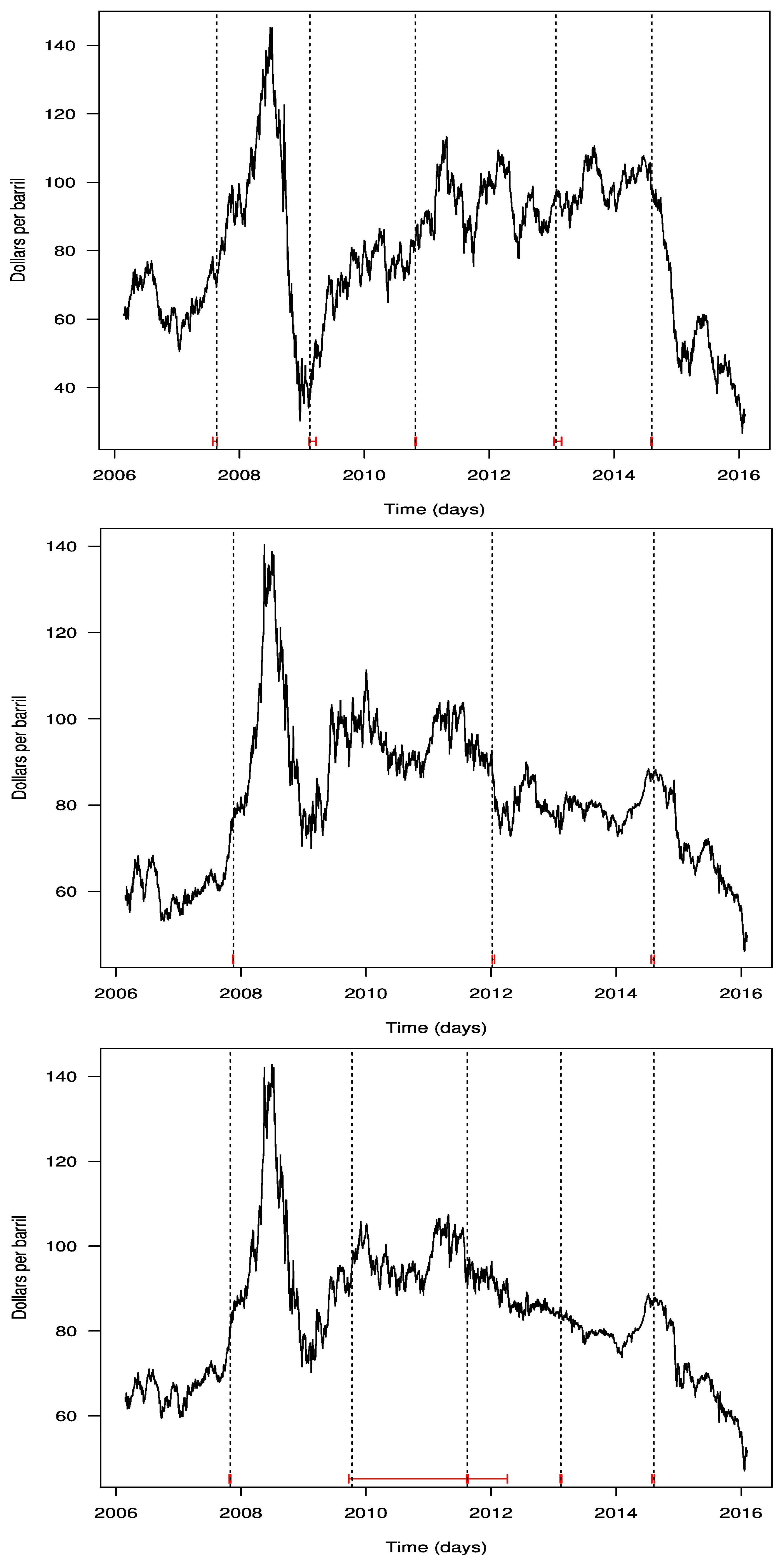
Figure 3 shows the lower volatility of futures contracts with long maturity periods on every day. Since 2008 these futures prices have been higher than spot prices when the latter have fallen considerably, and below them when spot prices have been very high.
Figure 3 also shows a peak of $145 and a rise in oil prices in July 2008. According to Kaufmann and Ullman [
4], this rise was caused by changes in market fundamentals and speculation. These authors conclude that the increase anticipated by prices set in futures markets, exacerbated by speculators, was transmitted to the spot market. On the other hand, in 2015 futures prices were above the spot price, reflecting a situation of contango in the market.
Table 3 reports the descriptive statistics for spot and futures prices obtained as the longest maturities and estimated by a stochastic model, Jarque-Bera test for normality (Jarque and Bera [
19]) as implemented in the R package
tseries (Trapletti and Hornik [
20]) as well as the Augmented Dickey-Fuller (ADF) unit-root test (Dickey and Fuller [
21]) as implemented in the R package
tseries (Trapletti and Hornik [
20]) with structural breaks. A first glance, the skewness shows that in all cases the data sets have a slight asymmetric probability distribution. On the other hand, the kurtosis values show that none of them have a value close to 3 (the theoretical value for a Gaussian probability distribution), except the log returns for the futures prices estimated by a stochastic model. However, the Jarque-Bera test indicates that none of the probability distributions of these time series appear to be normally distributed.
Table 3 also reports the results of ADF unit-root test for the levels of the series as well as the log returns. When the ADF test is applied to the raw data, we fail to reject to reject the null hypothesis for all the time series. Nevertheless, when the test is applied to the log returns, all nulls are rejected consistently. Thus, the test reveals that all the raw data sets are integrated of order one, that is, are non-stationaries whereas the log returns do not contain a unit-root indicating that these series are stationaries.
2.3. The Wavelet Methodology
Discrete Wavelet Transform (DWT) [
13,
14] is a mathematical tool that can handle non-stationary time series and which works in the combined time-and-scale domain. There are various algorithms for computing the DWT. In this paper we use the Maximal Overlap Discrete Wavelet Transform (MODWT) because of its advantages over the classical DWT. To begin with, the MODWT can tackle any sample size N, while the DWT of level J restricts the sample size to a multiple of 2J. Also, more importantly, the MODWT is invariant to circular shifting of the time series under study, while the DWT is not. Furthermore, both the DWT and MODWT can be used to analyze variance based on wavelet and scaling coefficients, but the MODWT wavelet variance estimator of the wavelet coefficients is asymptotically more efficient than the equivalent estimator based on DWT [
13,
14,
22]. The MODWT is used to compute wavelet variances, wavelet correlations (WC) and cross-correlations (WCC) of bivariate time series [
13,
14]. Several applications of the DWT and MODWT can be found in economic and financial literature (see e.g., [
8,
13,
23,
24]) and to a lesser extent in energy studies [
25,
26,
27]. Nevertheless, to date the WCC (via MODWT) has not been widely used to study the correlation and co-movements between spot and long-term futures oil prices (though some exceptions are discussed below).
Yousefi et al. [
9] propose the wavelet analysis approach as a possible vehicle for investigating market efficiency in futures markets for oil (prediction of oil prices). More recently, Naccache [
10], Aguiar-Conraria and Soares [
28], Benhmad (2012) [
25] and Reboredo and Rivera-Castro [
11], among others, address the question of the link between oil prices and the macroeconomy using world data and a time scale decomposition based on the theory of wavelets. However, the first study of the relationship between spot and futures prices of crude oil using wavelet analysis was not performed until 2015 by Chang and Lee [
12]. They investigate the time-varying correlation and the causal relationship between crude oil spot and futures prices using wavelet coherency analysis. Chang and Lee) [
12] find significant dynamic correlations between these variables in the time–frequency domain, in a such way that spot and futures prices contribute to the dynamics of the long-run equilibrium. They recommend that future studies focusing on the behavior of oil prices should consider the characteristics of the time–frequency space and lead–lag dynamic relationships. However, Chang and Lee [
12] use futures contracts with one, two, three, and four months, i.e., futures contracts with a very short-term maturity (around 0.33 years). They do not take into account the causal relationship between oil spot and futures prices. This task was tackled more recently by Alzahrani et al. [
15] in the first combined study that mixes wavelet analysis and non-linear causality. Alzahrani et al. [
15] find consistent bidirectional causality between spot and futures oil markets on different time scales.
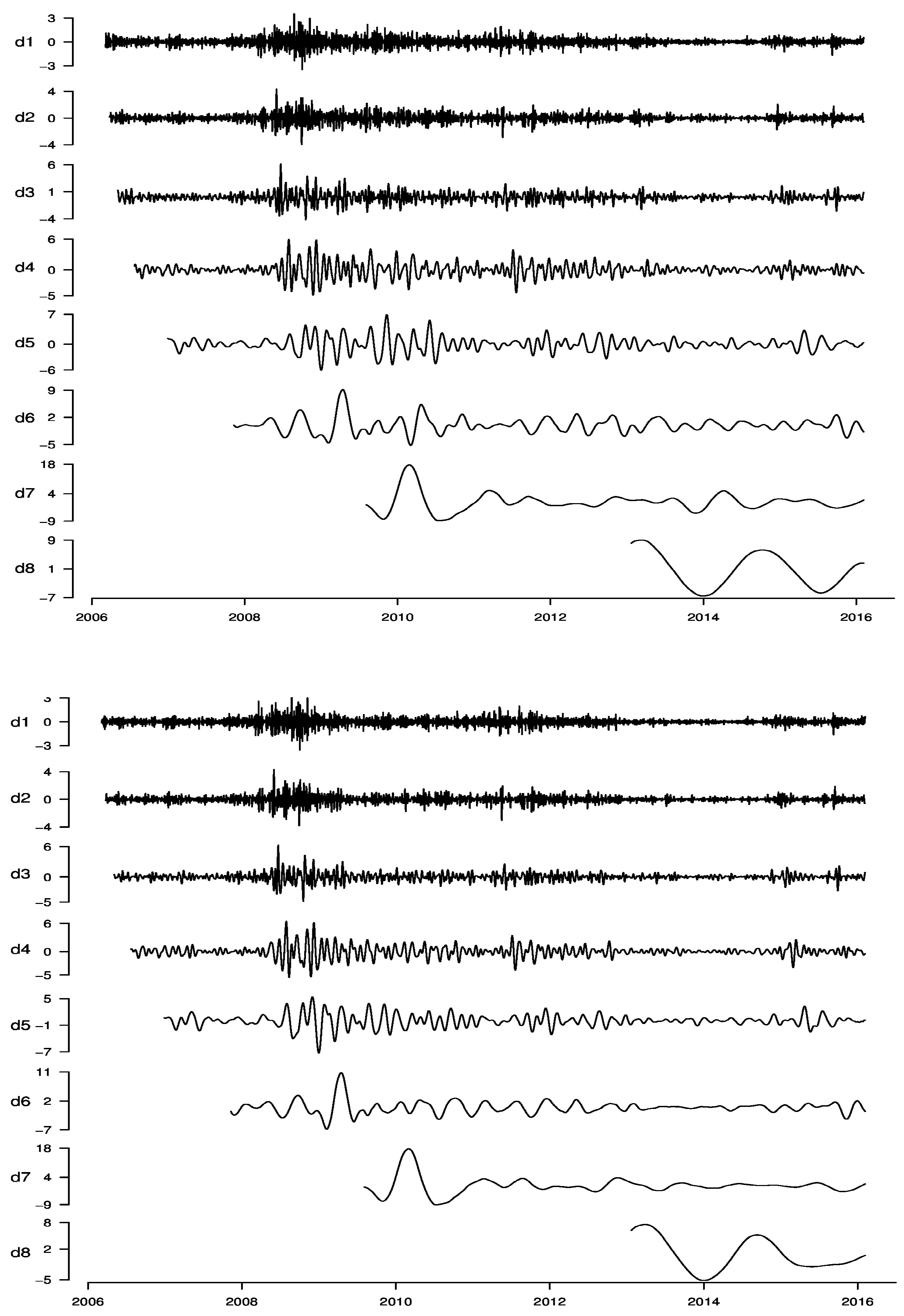
In order to decompose the daily oil time series (
Figure C1;
Appendix C) in this work, we have applied the MODWT with a Daubechies least asymmetric (LA) wavelet filter of length
L = 8, commonly denoted as LA(8) [
13,
29]. The maximum decomposition level
J is given by
[
13,
14], which in this case is
J = 8, so the MODWT produces eight wavelet coefficients and one scaling coefficient, that is,
and
, respectively.
Note that the level of the transform defines the scale of the respective wavelet coefficients
. In particular, for all families of Daubechies compactly supported wavelets the level
j wavelet coefficients are associated with changes at an effective scale of
days (in our case) [
23]. Moreover, the MODWT utilizes approximate ideal bandpass filters with bandpass given by the frequency interval
for scale levels 1
≤ j ≤ J. Inverting the frequency range and multiplying by the appropriate time units ∆
t (one day in our case) gives the equivalent periods of
days for scale levels 1
≤ j ≤ J [
29]. This means that in our case study, with daily data, the scales
,
j = 1, 2, …, 8 (associated with changes of 1, 2, 4, 8, 16, 32, 64 and 128 days) of the wavelet coefficients are associated with day periods of, respectively, 2–4 (includes most intraweek scales), 4–8 (including the weekly scale), 8–16 (fortnightly scale), 16–32 (monthly scale), 32–64 (monthly to quarterly scale), 64–128 (quarterly to biannual scale), 128–256 (biannual scale), and 256–512 days (annual scale).
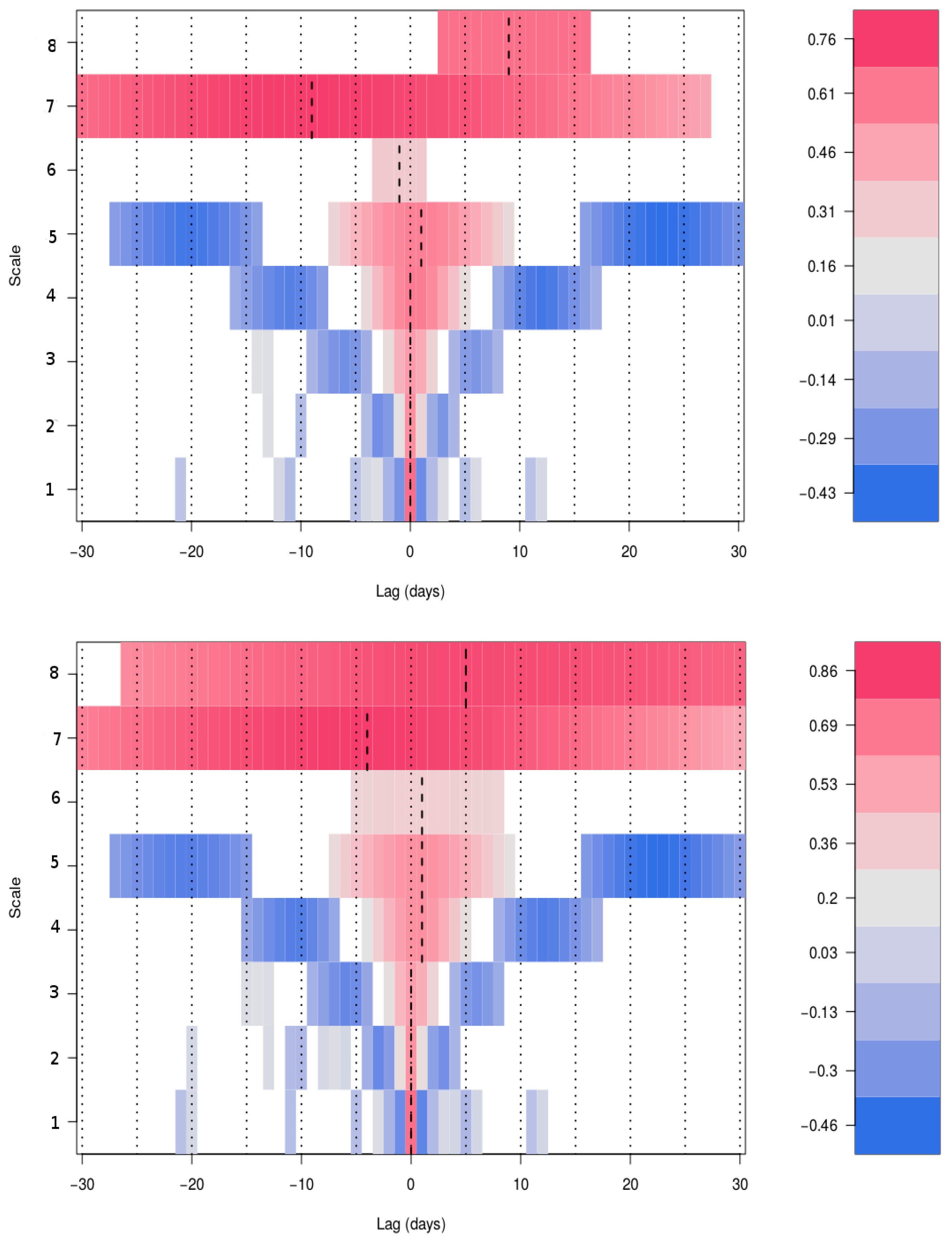
In order to analyze the relationship between spot and long-term futures prices from the crude oil market time series at different time/period horizons, we compute the wavelet cross-correlation (WCC). We follow the methodology for computing the wavelet transform (MODWT) and WCC given by Gencay et al. [
13], as implemented in the R package Waveslim [
30]. To obtain a graphical interpretation of wavelet correlation and cross-correlation analysis, we use the R package W2CWM2C [
17,
31].
The MODWT unbiased estimator of the wavelet correlation for scale
between two time series
X and
Y can be expressed as follows [
13]:
where
is the unbiased estimator of the wavelet covariance between wavelet coefficients
and
, and
and
are the unbiased estimators of the wavelet variances for
X and
Y respectively, associated with scale
. An unbiased estimator of the wavelet variance based on the MODWT is defined [
13] by:
where
is the
jth level MODWT wavelet coefficients for the time series
X,
is the length of scale
wavelet filter, and
is the number of the coefficients not affected by the boundary.
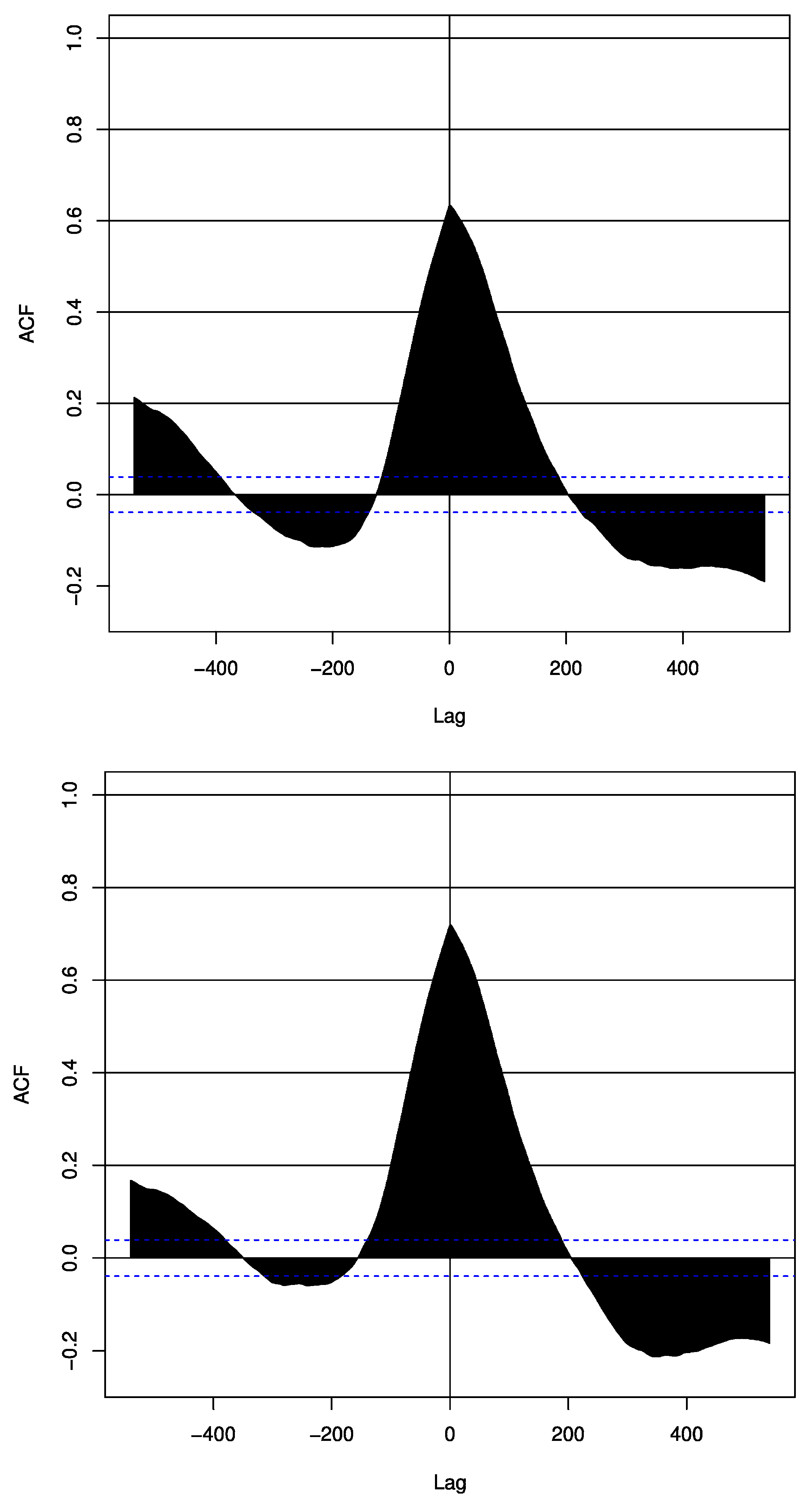
The MODWT unbiased estimator of the wavelet cross-correlation for scale
and lag
τ between two times series
X and
Y is defined by [
13]:
where
is the unbiased estimator of the wavelet cross-covariance, and
and
are the unbiased estimators of the wavelet variances of
X and
Y, respectively. Note that the WCC is roughly analogous to its Fourier counterpart, the magnitude squared coherence, but the WCC is related to bands of scales (frequencies) [
32]. The WCC
, and is used to determine lead/lag relationships between two time series on different scales
.
The confidence interval for the WCC is based on an extension of the classical result on the Fisher’s Z-transformation of the correlation coefficient [
32]. Thus, an approximate 100(1
2p)% confidence interval for the WCC is given by
, where
,
is the 100p% percentage point for the standard normal distribution, and
[
13,
32].
2.4. Nonlinear Causality Tests
Savit [
33] argued that financial and commodity markets are dynamical systems that could manifest nonlinearities, and he also argued that these elude common linear statistical tests (including linear causality tests). Baek and Brock [
34] proposed a nonparametric test for detecting nonlinear causal relationships based on the correlation integral, which is an estimator of spatial dependence across time. Later on, Hiemstra and Jones [
35] provided an improved version of Baek and Brock [
34]. However, despite the test of Hiemstra and Jones [
35] is (probably) the most used nonlinear causality test in economics and finance (there are others nonlinear causality tests developed to analyze this kind of data, but these are not commonly used, e.g., Bell et al. [
36]; Su and White [
37]; among others). However, it tends to over-reject the null hypothesis if it is true (Diks and Panchenko [
16,
38]). For this reason, Diks and Panchenko [
16] proposed a new nonparametric and nonlinear Granger causality test to avoid the over-rejection. In our work, we use the causality test of Diks and Panchenko [
16], as implemented in the C program
GCTtest, which is freely available on the Internet [
39]. In addition, we use the test of Toda and Yamamoto [
40] only to analyze potential causal relationships in raw data. This test is implemented in the R language and it is available freely on the web [
41].


