1. Introduction
In the global perspective of electric energy usage, lighting’s share reaches 19% on a global scale [
1] and 50% on a Europe-only scale [
2]. For that reason, decreasing this consumption is at least as important as the development of new methods of energy generation. This reduction (negawatt power) has a strong influence on the efficiency of an electricity grid structure for two reasons:
It is made on the user side so one avoids power losses during transmissions between generation and lighting installation,
It is carried out during the energy peak hours, in comparison to major renewables such as wind turbines or photovoltaic (PV) panels which are nondeterministic.
The number of streetlights in the European Union was assessed by the European Commission as more than 90 million traditional streetlights (
i.e., non-solid state light sources) in 2013, with over 75% of the installations being older than 25 years [
3], which means that they should be replaced with new fixtures. Solid State Lighting (SSL) technology is crucial for our purposes because it enables a dynamic control of illuminance level. Current SSL market penetration in Europe is very low: the LED (Light-Emitting Diode) market share (in value) reached 6.2% in 2010. Several studies predict that SSL will account for more than 70% of the general European lighting market by 2020 [
1].
The above numbers show that even a small improvement in the unit power efficiency scales to significant values of an overall reduction. To benefit from this potential of available power savings, one can use a range of approaches which may be divided roughly into the following groups:
Retrofit: replacing HID (High-Intensity Discharge) (e.g., mercury-vapor, sodium-vapor, metal-halide) lamps with LEDs.
Design: optimization based on a uniformed street layout, ”customized” optimization relying on accurate coordinates (e.g., GIS (Geographic Information System)-based) of the road and luminaires.
Control: dimming and scheduled dimming, scheduled lighting class reduction, adapting dimming level to an actual environment state, others.
Other, unclassified methods, e.g., improving reflective properties of a road surface.
Due to improvements of the lighting system components based on LED or OLED (Organic Light-Emitting Diode) technology, retrofitting allows us to reduce the energy consumption by at least 40% [
4]. Due to the extremely low onset time of LEDs and the flexibility of photometric solid shaping, they are perfectly suited for a lighting design and for building advanced control systems, contrary to HID light sources. In particular, LEDs can be dimmed so an applied power level can be adjusted precisely to the actual needs determined by a state of an environment (traffic level, outdoor lighting and so on) and constrained by mandatory lighting standards [
5] (a luminous flux intensity is nearly linearly dependent on the power being applied (Some side effects of a fixture’s high dimming is growth of a reactive power. It will not be discussed here, however). A dimming level depends on the road classification (highway, residential area, bike lane) which can additionally change due to the variable traffic intensity. Another factor influencing this classification is the ambient light level.
An intelligent system which controls and optimizes a lighting installation’s behavior is, in a natural way, the element of a distributed electricity smart gird [
6,
7] which can reduce the energy consumption by several percent. Technical problems with lighting design preparation such as a a real-time control system has been considered in [
8], but the basic issue is the preparation of multiple variants (practically counted by hundreds) of each lighting scene, corresponding to different predefined environment conditions. Unfortunately, designers using, for example, the popular DIALux software (or other, similar programs), prepare a project containing 1000 lamps in one week of time. It becomes obvious that creating 100 additional variants of this project is infeasible due to the expected cost and preparation time. Thus, it is crucial to support a designer by providing an AI (Artificial Intelligence) system capable of building such a project in a reasonable time.
One of the first non-standard attempts of making a lighting design [
9,
10] does not consider luminous flux dimming and still has a limitation of high execution time. The niche methods such as increasing reflectance of a road surface in tunnels [
11] will not be discussed here either due to their limited area of application. Instead, the focus will be put on design methods which are not so common as retrofit and control, which is caused by their computational complexity.
An interesting approach to improving energy efficiency is based on rules of thumb giving relations among configuration parameters of an optimal installation such as spacing, fixture inclination angle or mounting height [
12]. For now, however, this approach is intended for discharge lamps only. Moreover, as a rule of thumb, it can produce suboptimal solutions instead of optimal ones.
In this article, the new, computational intelligence-based approach is proposed: it is assumed that lighting system components and their relationships are represented in some formal way so that the computing systems can solve a design problem fully automatically using exact coordinates of luminaires and illuminated areas (roadways, squares, etc.). Thanks to this, a lighting installation being designed is characterized by the high power efficiency (over-illumination is minimized) and, on the other side, all standard-based performance requirements are met.
The presented idea is based on the following requirements:
The proposed formalism has to have the sufficient expressive power to describe all analyzed objects and relationships among them.
It will be possible to build either exact or effective heuristic algorithms capable of finding the best (local) solutions.
The proposed formalism will support application of the above algorithms in parallel computations to achieve a final result in an acceptable time.
The article is structured as follows. In
Section 2, the various aspects of lighting design creation are discussed. Particular attention is paid to constraining requirements (imposed by standards and best practices), control and computational complexity.
Section 3 introduces the hierarchical hypergraph model as being a formal representation of a lighting system and a framework for its analysis is performed with the help of a multi-agent system acting in parallel. The links between a model and physical objects being represented are also described. The scheme of the model application is presented in
Section 4. The case study of a real-life model application can be found in
Section 5. In
Section 6, energy savings obtained for other practical applications are presented. Final conclusions are placed in
Section 7.
2. Roadway Lighting Design Task
In this section, a brief overview of an outdoor lighting design process is given to define the context for future considerations.
The designer’s objectives are threefold: ensuring compliance with mandatory standards, good practices and recommendations [
5,
13], optimizing a design with respect to some measurable criteria like energy-efficiency, investment costs or payback period, and achieving some subjective goals (e.g., aesthetics). Note that those three objectives have to be achieved jointly.
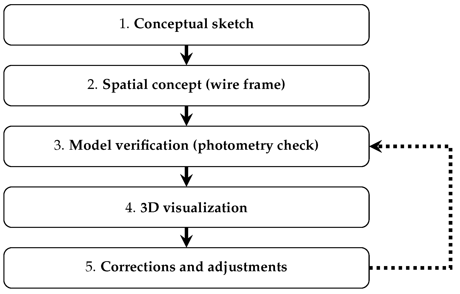
Usually, a human-made preparation of a project is supported by some photometric verification capable software like DIALux. A design process may be structured in the way shown in
Figure 1. Note that the trial-and-error nature of a process is reflected by the loop iterating through steps 3 → 4 → 5. The loop execution is continued until three objectives defined previously are achieved.
Due to the great number of available variants corresponding to such factors as positioning of objects, material selection and so on (see the example shown in
Table 1), a designer has to use, besides his expert knowledge, the trial-and-error design method. Even assuming that the experience in a domain allows for reducing a number of possible scenarios, the search space size and design time still remain large. It also has to be mentioned that lighting situations are simplified in the practice to accelerate the design process. This simplification is achieved by averaging luminaire spacings, road widths, pole setbacks, and so on. In addition, the presence of buildings, trees and other similar objects is neglected.
The schema presented above is characterized by the high work overhead, especially for restrictive optimization criteria, e.g., related to the power consumption (exploitation costs) and a human performance is a bottleneck of this process.
The core requirement which has to be addressed in lighting design is the compliance of a project with mandatory standards for illumination, defined for various areas such as roadways, driveways, intersections, sidewalks
etc. For each of them, an appropriate lighting class is assigned [
14] depending on the traffic characteristics: dominant user types, traffic flow intensity, average speed of vehicles
etc. For each lighting class, the performance requirements are assigned. For example,
Table 2 shows so called ME-lighting classes which establish performance requirements for traffic routes of medium to high driving speeds as defined in the European standard EN 13201-2 [
5]. Similarly, performance requirements are defined for road intersections, conflict areas and others.
The specific field where a lighting design plays a crucial role is lighting control. One of the important approaches to the dynamic (it should not be confused with static methods such as a performance scheduling) street lighting control is adapting a lighting class (and thus an installation’s performance requirements) to the actual traffic intensity reported by sensors. Other factors, e.g., weather conditions or pedestrian traffic, should also be taken into account when adjusting a performance to an environment state—what additionally increases the complexity of a lighting design process.
Let be a discrete, finite set of values of a given environment property, , impacting the class selection, where and . Then, it is obvious that the total number of states (profiles) for which a performance has to be pre-calculated is . Additionally, a presence of objects reflecting or screening a luminous flux (buildings, trees) can be considered.
For simplicity of presentation, we consider the influence of traffic flow intensity on the lighting intensity level only.
Table 3 shows lighting classes for actual flow values (note that a daily flow can be updated every 15 min) and the corresponding relative power usages (For the street examined in the Smart Power Grids project, financed by the Polish National Fund for Environmental Protection and Water Management [
15], it was proved that for a 24-h performance structure ME2-51%, ME3b-25%, ME4a-24%, the power usage reduction at the level of 20% is achieved). Environment state change events are reported to the lighting control system either from a telemetric layer or from other sources such as BTS-based (Base Transceiver Station) monitoring facilities [
16]. Such a control system imposes on a design process the need of a prior preparation of multiple setups of a lighting installation, covering all combinations of lighting classes and ambient light levels—the additional motivation for automating a design process.
It should be stressed that the presence of buildings, trees and other light obstructing objects also influence selection of a lighting class due to the impact on the difficulty of navigational tasks and complexity of visual field [
14].
As an alternative to the approach discussed above based on uniformed street and luminaire layouts, we propose preparation of a project, performed by a software system, relying on the accurate inventory data (poles’ locations and heights, street geometry data, fixture models and so forth) and a set of criteria defined by a human designer. Such a method referred to as the
customized design is shown to yield important energy savings compared to the typical approach [
17].
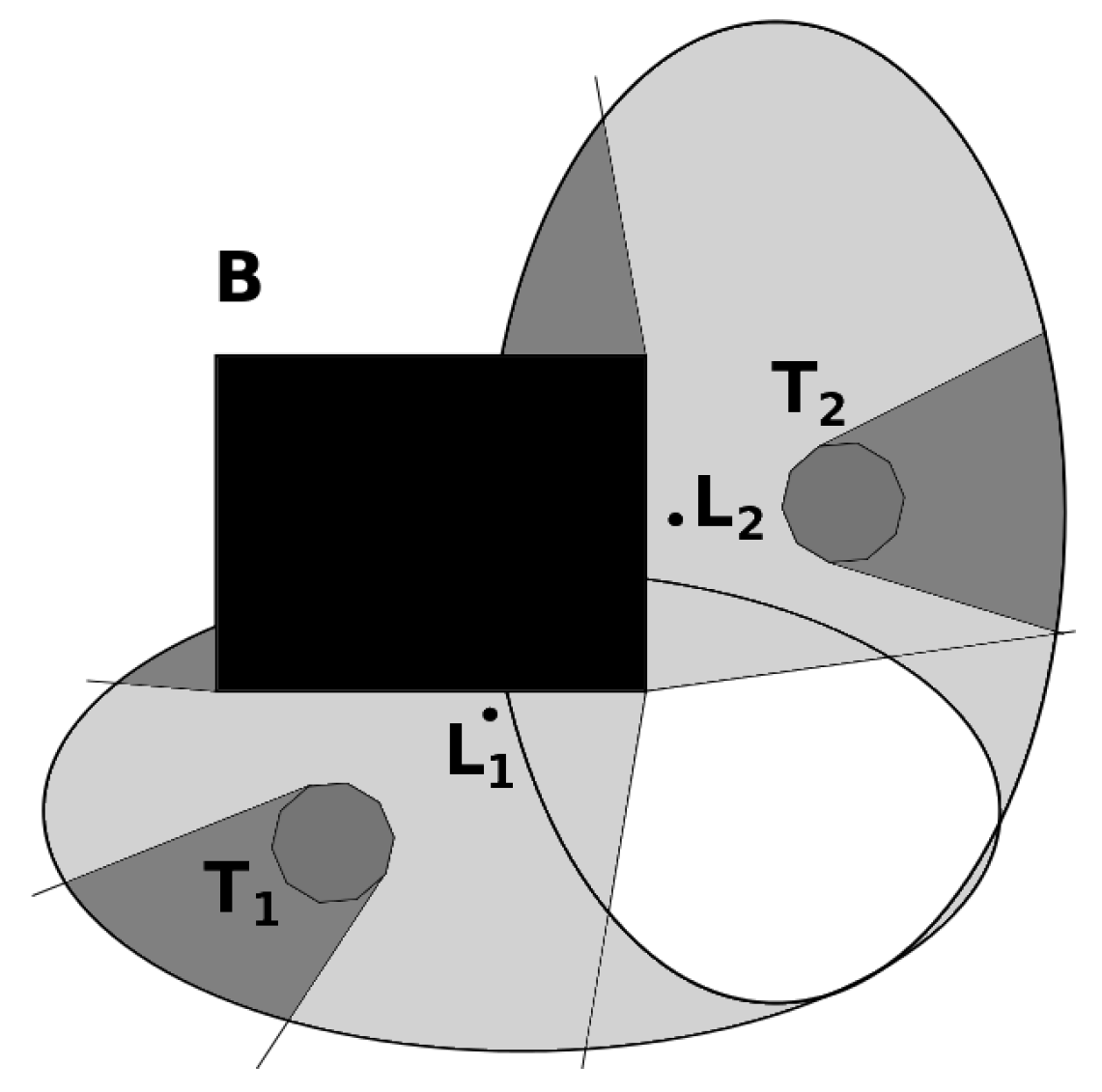
A customized design process starts with a scene containing several types of entities attributed with a complete set of properties required by a designer. The following list contains particular types and sample attributes of entities (see
Figure 2).
Buildings and other massive objects—size, coordinates, reflective properties of the surface (if applicable), main functionality.
Small objects, e.g., street furniture, trees, bushes—location coordinates, geometry, reflective properties of the surface (if applicable).
Areas which can be distinguished on the basis of their functionality: roadways, driveways, intersections, sidewalks, squares, and so on—size, layout, coordinates, reflective properties of the surface, functional properties (traffic flow rate, main user type, max. allowed speed), lighting class.
Luminaires—coordinates, post type/height, spacing, arm length, fixture model, photometric solid (a luminous flux distribution), other fixture’s properties.
It has to be remarked that elliptical shapes of illuminated areas shown in
Figure 2 are the samples only. In fact, such a shape depends on a photometric solid and a fixture’s orientation. Note that during the optimization process both properties (e.g., photometric solid and orientation angles) can be adjusted.
Regarding the above list and assuming that degrees of freedom in the solution search process are given in
Table 1, it may be easily computed that the number of variants to be checked for a new installation design is equal to 12.54 × 10
6.
The basic assumption underlying the design process automatization is that one is able to build a formal model for solving a design problem. Such an assumption is necessary because only a precise problem specification is understandable for computers. The most suitable formalism for this purpose is the graph-based one. It is well suited for design purposes and enabling substantial reduction of a design preparation time. The idea of applying a graph representation for overcoming complexity issues is not new. Kreowski [
18] proves, for example, that the Hamiltonian path problem can be solved in polynomial time using graph multiset transformations (unfortunately, no efficient implementation of the graph multiset formalism is known).
It has to be noted that the proposed workaround to complexity issues can be also applied to other types of lighting such as illumination of tunnels, stadiums
etc. In particular, it applies to indoor lighting design. It is possible because there exists a hypergraph representation of internal spaces [
19]. Such a formalization enables automation of a design process. Bulk optimization of indoor lighting will be considered in future research.
3. Hierarchical Hypergraph Representation
The entire considered scene being designed and consisting of buildings, objects, footpaths, roads and other areas will be described by means of a hierarchical hypergraph representation (see
Figure 3) similar to the concept of a HD-graph (hierarchical distributed) introduced by Taentzer [
20].
The upper level of the hierarchy is modeled as a graph with nodes corresponding to objects and areas enumerated in
Section 2 and edges representing spatial and logical relations among them (
Figure 3a). The upper level representation can be viewed as a coarse grain description of a scene. For a smart lighting system, like this one developed within the Smart Power Grids project (discussed in
Section 5), it contains not only the nodes representing "massive" objects (buildings, areas) but also those corresponding to sensors, control cabinets or relevant network infrastructure components. Another important piece of data contained at this level are traffic intensities for subsequent roads, and influences of particular luminaires on given areas or buildings.
The nodes of an upper-level graph encapsulate hypergraphs belonging to the lower level of the representation (
Figure 3b), modeling 3D objects and any surfaces (areas) as well [
21]. To facilitate further computations, an upper level graph is subject to a decomposition process transforming it into a
slashed graph (
Figure 3c) introduced in Definition 3. A slashed graph is the environment supporting parallel computations performed by a multi-agent system.
In the following subsection, the lower level hypergraph model will be defined.
3.1. Lower Level: Hypergraph Model of Solid
Suppose an object (solid) consisting of faces, physical edges and physical vertices (contrary to graph edges and graph vertices) is given.
Table 4 shows the correspondence between its elements and hypergraph components. Definition 1 introduces a formal hypergraph representation of a solid.
Definition 1. An S-hypergraph (solid hypergraph)
of an object S is a tuple of the form
where
N is a nonempty set of nodes,
is a set of edges,
is a set of hyperedges,
for
is a labeling function for vertices, edges and hyperedges, respectively, with a corresponding set of labels
;
for
is an attributing function for vertices, edges and hyperedges, respectively, with a corresponding set of attributes
.
It is assumed that dimensionless objects like luminaires or sensors can be modeled by appropriately attributed nodes attached to the regular ones, representing faces. For example, the luminaire node is a neighbor of a certain node representing the surface on which this luminaire is located, i.e., .
Note that adding the supplementary edges may be considered here. For example, in the case of a dynamic, smart lighting system, one takes into account a luminaire’s light reflected from a building face. At the level of a graph model, it corresponds to an edge connecting a luminaire node, , with a relevant face node . Contrary to the previous example, the luminaire L does not need to be attached to the face F.
The detailed formalism underlying hypergraph modeling of solids may be found in [
21]. The important capability of the model is representing curved physical edges and faces of solids. It is viable thanks to attributing functions which can store advanced geometric features of objects.
To enable application of hypergraphs to surface modeling, one assigns an infinitesimal height ϵ to a surface A and then proceeds as with a regular solid.
3.2. Upper Level: UL-Graph and Its Slashed Form
Decomposition of a main (central) calculation task, represented as a graph, into the particular subtasks produces a set of the upper level objects. Thanks to their small sizes (no detailed information needs to be stored in a node at this moment), a multi-agent system operates on a lightweight structure which can be enriched instantly in the on-demand mode as soon as any detailed data are required for further computations—for example, when an agent moves to the lower level.
Having the notion of an S-hypergraph defined, one is ready to formalize the upper level of the hierarchical model.
Definition 2. UL-graph (upper level graph) is a triple where V is nonempty set of nodes such that each a node represents some S-hypergraph, is a set of directed edges, is a labeling function, and denote sets of node and edge labels, respectively, and A is a set of edge attributes. The family of UL-graphs will be denoted as .
We set the edge structure to to store all required data in edge attributes. These data include slashing details (e.g., geometric coordinates) but also problem specific information (e.g., architectural details of adjacent buildings). In particular, some attributes hold detailed information describing binary relations between faces of two hypergraphs hosted by relevant . The UL-graph definition can be also extended, e.g., by introducing an attributing function for nodes, but such an extension does not impact further considerations so it will not be considered here.
A UL-graph formally describes a lighting scene that enables computer aided searching for an optimal setup of a lighting installation. The high computing complexity of a design process enforces introducing parallel processing. Thus, computations can be completed in a reasonable time.
The concept of a slashed form of a UL-graph
G aims at distributing
G in such a way that coupling among resultant subgraphs, in terms of shared elements, is minimal. Thanks to this, a distributed processing performed for example, by a multi-agent system is not throttled by the communication overhead. To achieve this, graph edges are split in a reversible manner. The detailed analysis of the computational complexity for such a distributed system is presented in [
22].
Definition 3 (Slashed form of
G). Let
. A set
of graphs is defined as follows:
and , where is a set of core nodes, denotes a set of dummy nodes and ,
where are mutually disjoint for ,
such that is the replica of v; ,
is incident to, at most, one dummy node.
An edge incident to a dummy node is called a border edge. The set of all border edges in
is denoted as
. A set
is referred to as a set of core edges of
. Let
, then a set
as defined above is referred to as a slashed form of
G, and denoted
, iff following conditions are satisfied:
(α denotes an isomorphic mapping between graphs) and are disjoint for .
—a bijective mapping such that (i) , (ii) is a replica of and . is called a slashed edge associated with replicated dummy nodes .
(i) for some i, such that or (ii) for some , such that e is a slashed edge associated with v and .
is called a slashed component of G.
Note that f mapping recovers labeling/attributing data of a slashed edge based on labeling/attributing of relevant border edges.
Remarks. (i) To preserve the clarity of images, attributing/labeling of graph edges in figures will be neglected. (ii) A border edge incident with a dummy vertex v will be denoted as . Similarly, a border edge incident with a dummy node indexed with an index will be denoted as . (iii) It is possible to slash a core edge to a pair of border ones in such a way that a dummy node d refers to the same physical entity as x does—in particular, when and d represent points of or space. Thus, using a slashed representation does not generate additional geometric data related to a slashing point.
The possibility of splitting a large graph into several subgraphs allows performing parallel computations in a multi-agent environment (each subgraph is maintained by a single agent) with synchronization protected by moving partition boundaries among subgraphs (see [
23]).
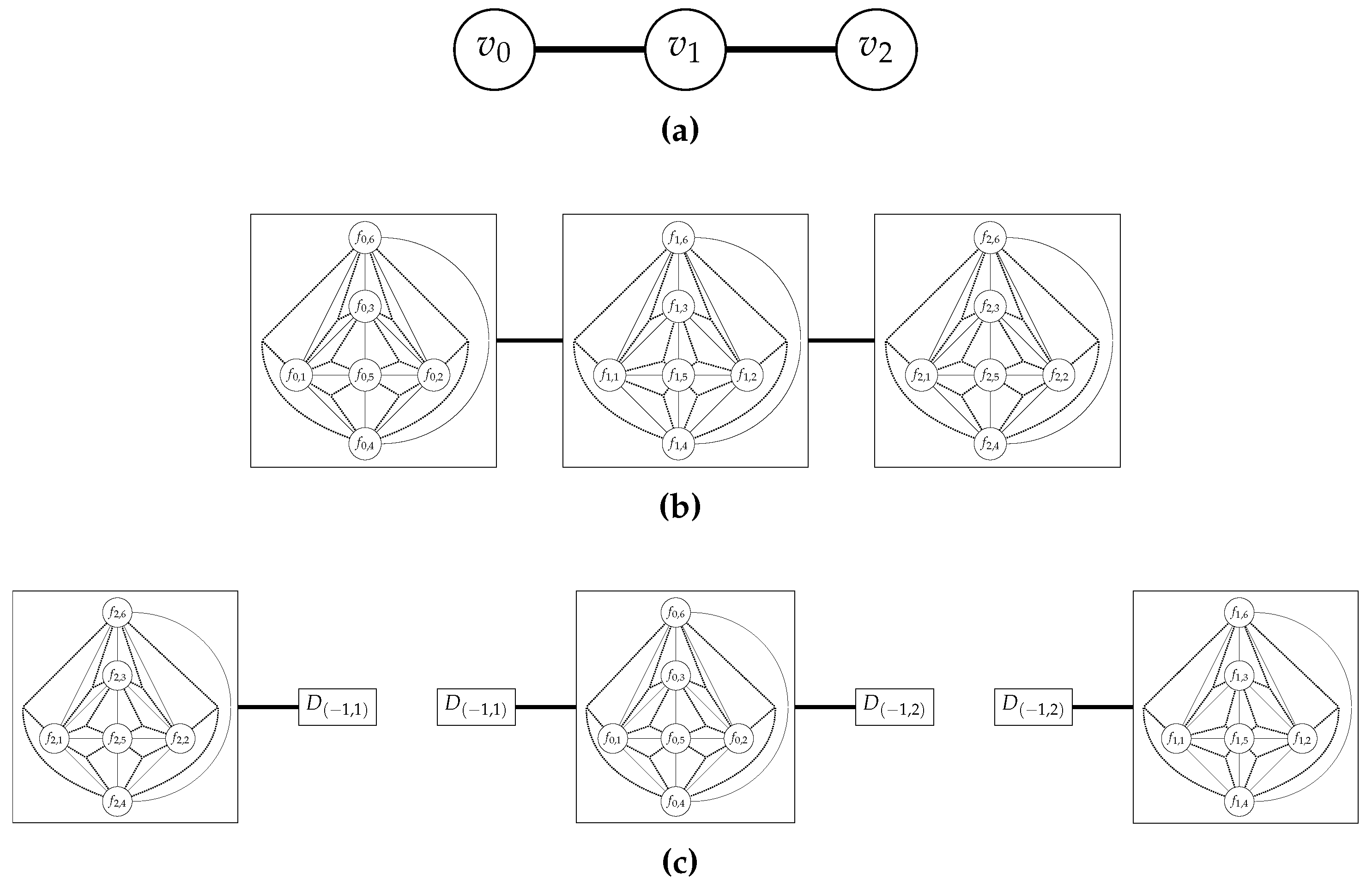
Figure 3a shows the UL-graph
G representing three adjacent cuboids. Thick edges represent the relation of adherence of solids. In
Figure 3b, the lower level perspective is shown: each node of the UL-graph is expanded into the S-hypergraph. Finally, in
Figure 3c, the slashed form of
G is presented. Such a low-level distributed form of a graph representation is ready for a multi-agent system deployment.
4. Application of the Model
Optimizing configuration of a lighting installation is automated in the following steps:
Extracting segments of a scene.
Establishing S-hypergraphs for particular segments (the lower level of the model).
Migrating to the upper level of the model and decomposing a UL-graph into the slashed form.
Deploying agents in a distributed UL-graph.
Parallel optimization of a lighting installation configuration performed by a multi-agent system.
Assembling results.
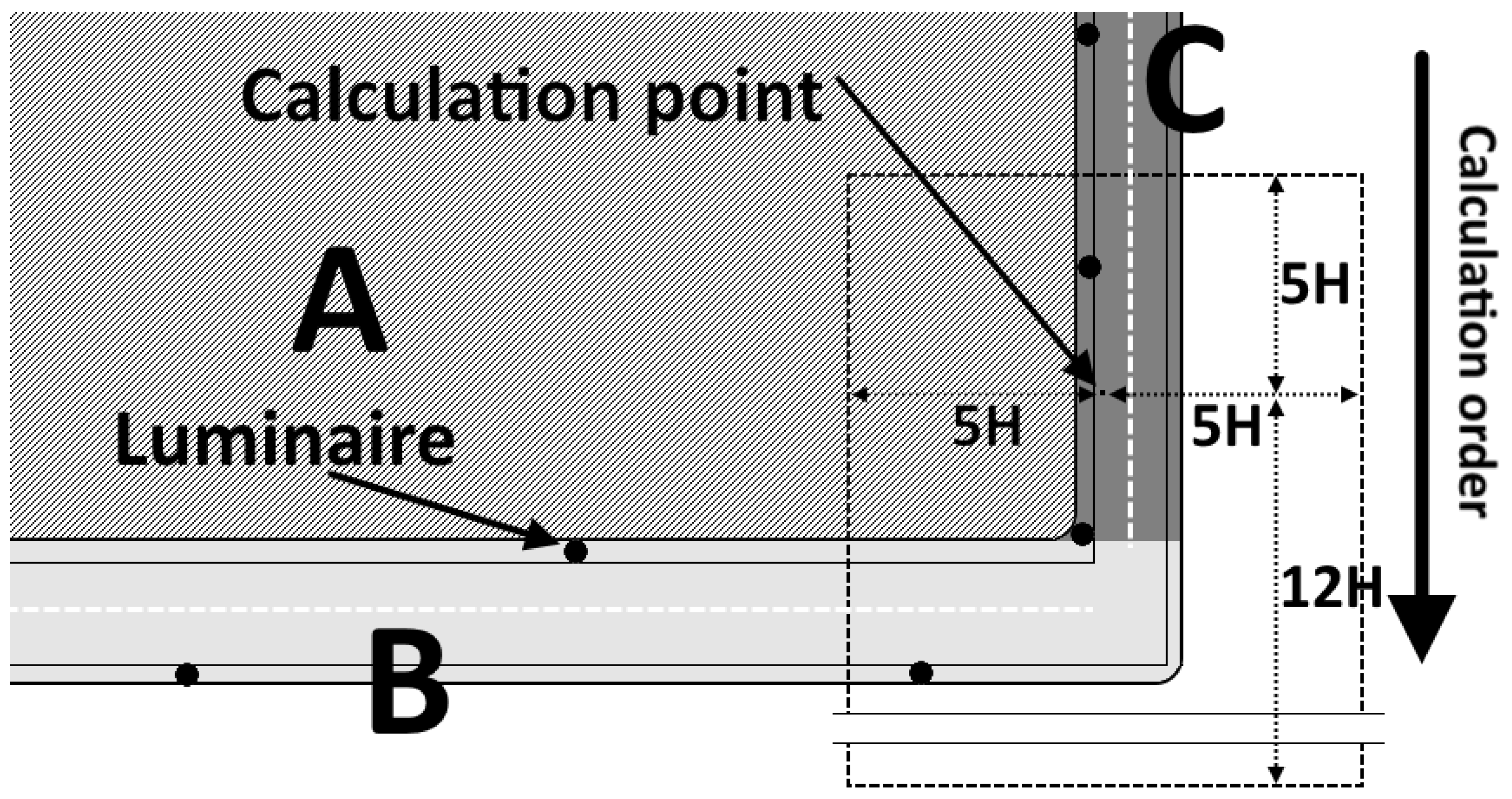
To demonstrate the mechanism of the model application, a retrofit of a lighting installation is considered. Let us assume that the relevant scene shown in
Figure 4 is given. It consists of two perpendicular roads and the neighboring building. Moreover, two rows of luminaires are located along them. Additionally, it is assumed that, for each luminaire, the following attributes are maintained: (i) fixture related data, (ii) coordinates, (iii) post height, arm length, (iv) references to neighboring S-hypergraphs.
The scene is decomposed into three sections: building (A) and two roads with adjacent sidewalks (B and C respectively). It is assumed that lighting classes for the roadways B and C are, respectively, ME3a and ME4a (see
Table 2).
Thanks to the distributed, slashed graphs-based representation, which enables an efficient synchronization and thus the parallelization of computations, a multi-agent system can perform a design process in parallel. To each of the above sections, a computing agent is assigned. An agent’s goal is finding such parameters of an installation (fixture model, dimming level, post height and arm length) that the resultant power usage is minimal and lighting class requirements are satisfied.
To determine the performance of an installation, an agent has to make photometric computations [
24] for subsequent roadways included in its section (in the example, the single road for both B and C). To accomplish that, for each calculation point, all luminaires falling into a zone of size 10
H × 17
H around it have to be taken into account, where
H is a pole height (see
Figure 4).
Note that some part (some calculation points) of the street C is screened by the corner of the building (located in the section A) which blocks the luminous flux outgoing from the bottom luminaires. In such cases, the agent maintaining section C gathers all necessary information concerning a given fixture to determine an impact of the building A on the light distribution.
Another factor to be taken into account is the impact of the light outgoing from luminaires located on the roadway C and reflected from the surface of the building A. This impact, in turn, is calculated on the basis of reflective properties of a relevant face of the building, which are obtained from attributes of a S-hypergraph associated with A.
After collecting all data required for photometric computations, the agents start searching for a solution. This process is based on time efficient, heuristic methods [
17]. The important computational question is related to cooperation among agents, e.g., in the case of areas influenced by luminaires belonging to two or more sections. In such a situation, agents have to find some lamp adjustments acceptable for all parties: usually the most "restrictive" ones.
5. Case Study
The problem of finding the optimal configuration of a lighting installation was considered in the Smart Power Grids project, mentioned in
Section 1.
Within this project, all photometric calculations were performed luminaire by luminaire with precise GIS data provided. The power reduction achieved thanks to applying this approach varied between 10%–15% depending on the scene being considered, compared to standard lighting design methods. Note that this comparison was possible because computations performed according to the "standard" approach were executed using a graph-based heuristic engine capable of making bulk photometric calculations. In this case, we had to apply the massive parallel computations to solve the problem in the acceptable time.
5.1. Project Description
The project was aimed at retrofitting a part of the road lighting infrastructure in the city of Kraków, Poland. In particular, it covered replacement of 3748 high-intensity discharge (sodium vapor) lamps attached to 73 control cabinets and distributed along 239 streets, for LED ones. Due to the variable properties of particular streets, they were subdivided for computational purposes into 622 uniform calculating segments. Each segment was assumed to comply with the following uniformity requirements:
Road width is either constant or varies within with an acceptable margin.
Luminaire layout is either uniform or varies slightly (in terms of varying spacings or setbacks) with acceptable margins.
At a given instant of time, one lighting class applies to the entire segment (i.e., the same performance requirements apply to its entire area).
An important aspect of the project was control, which was understood as performing appropriate actions (dimming selected luminaires/group of luminaires) in response to changing environment conditions reported by the telemetric layer (
i.e., sensors). The control mechanism was implemented with the help of lighting profiles (see
Section 1): transitions between subsequent environment states were triggering appropriate lighting profiles on particular segments.
To accomplish the above approach, 3 lighting profiles were ascribed to each calculating segment. The impact of an ambient light was neglected.
5.2. Graph Model
The applied graph representation of the problem relied on the presence of three types of physical/logical objects crucial for the system behavior: (i) segments, (ii) luminaires, (iii) telemetric layer components (induction loops, rain sensors,
etc.). The entities of those types are linked by following relations:
neighborhood (segment–segment),
impact on an illuminance level (luminaire–segment),
membership of a detection area (sensor–segment).
On the basis of the above, a UL-graph
modeling the system was defined (see Definition 2), where:
The set of nodes , where nonempty and mutually disjoint sets represent respectively segments, 3D objects (e.g., buildings), luminaires and sensors.
The set of edges , where contains undirected edges representing a neighborhood relation, contains directed edges representing a luminaire impact on a segment illuminance, and contains directed edges representing membership of the area covered by a sensor.
is the attributing function described in
Table 5.
Remarks. (i) Nodes of are aggregating ones in the sense that they represent potentially complex objects which may be modeled with S-hypergraphs. Other nodes are trivial, i.e., they correspond to dimensionless entities (or which structure may be neglected). (ii) Note that edges belonging to are generated in the course of computations as they require analysis of a geometric context data contained in . In particular, it refers to relationships among luminaires and neighboring buildings that can shade the road area.
5.3. Calculations
The elementary calculation step is determining resultant lighting performance obtained for the selected values of installation’s adjustments such as dimming level, pole height, photometric solid and others. The performance is described by five photometric quantities [
5,
25] (see
Table 2) being calculated in the step.
In an optimization process, this elementary step is repeated iteratively for all subsequent values of adjustments to achieve the optimal solution, implying the lowest power usage and keeping standard performance requirements satisfied.
Computations for a given segment were performed according to the following scheme.
- Phase 1
The optimal configuration yielding a minimal power consumption was found. It covered such parameters as pole height, arm length, photometric solid rotation angles and dimming ratio. The search process was performed against a dominant lighting class, i.e., a class which has the largest share in an installation work cycle. It should be noted that none of the above parameters, except the dimming ratio, may be changed in the next phase.
- Phase 2
The appropriate dimming ratios were determined for other lighting profiles. As mentioned above, the remaining parameters got immutable after completing Phase 1.
For such a computation scheme, 2087 optimization tasks were obtained: 696 for Phase 1 and 1391 for Phase 2. Thanks to applying the formal model of the system, based on the concept of a hierarchical distributed graph representation, the automated problem decomposition and the subsequent computations were doable. Computations, which were made on four-core CPU (Intel CORE i7), took 4 h 47 min compared to 13 h 12 min in the centralized approach case.
Note that one can easily assess the computation time for the greater number of cores, say 16. Let
denote the time required for decomposing a task into four subtasks and let
Y be a time required for processing a graph
;
Y is supposed to depend linearly on a graphs’s order:
. Then
. It is known that:
Taking into account the above one obtains straightforwardly that the total (including task decomposition) computing time for 16 cores will be of the order of 2 h and 39 min.
5.4. Dynamic Control
The dynamic control implemented in the Smart Power Grids project [
15] relied on adjusting lighting classes and a lighting performance to actual traffic flow intensities reported by inductive loops.
Due to the number of segments and a broad range of their lighting characteristics, the assessment of achieved savings will be presented in the aggregated form. The histogram of numbers of lighting profiles per segment is presented in
Table 6.
The interpretation of the table is the following. Let us consider the column with a value of 3–226. It means that 226 segments had 3 profiles ascribed, i.e., performances of 226 corresponding installations were adjusted to three different levels in the 24-h period (except switching off). In the scale of the entire area covered by the project, it generated the savings at the level of 15%.
For all of those profiles, the full photometric computations were calculated to prepare the adjustments suitable for a given lighting class.
6. Energy Savings
The problem of finding the optimal configuration of a lighting installation was also considered in other projects. It has to be noted that configuration refers to the set of properties of an installation including, among others, the post height, average luminaire spacing, fixture model, inclination and dimming.
The first optimization problem was considered in the project
Products and Services of a Living Smart Energy City Lab [
26]. The goal was reducing the over-illumination generated by street lamps (approx. 1950 luminaries, high pressure sodium fixtures) in Flemish cities. The number of available configurations enforced using parallel processing to the solution finding. The extremely simple structure of scenes allowed applying slashed representation only without further granulation. Due to the technological limitations of HID, light sources related to dimming capabilities, the optimization of configurations yielded statistically power savings at the level of 6%.
The next problem was preparing an energy-efficient lighting design prior to the planned retrofit of 5500 street luminaries (replacing high pressure sodium lamps with LED ones) in the city of Kraków, Poland, sponsored by the National Fund for Environmental Protection and Water Management (the Metropolitan Lighting Systems project). In this case, we dealt with more complex roadway layouts than previously, with variable functionalities including pedestrian zones, conflict areas (road intersections), and so on. They were grouped into 437 calculation fields. Additionally, the particular luminaries were assigned to 168 control cabinets, and the applied formal model had to address the problem of a control system architecture. The slashed graph model allowed to describe both the physical infrastructure of the system and its internal relationships as well but also allowed for finding the optimal solution in the time of several hours. A human designer workload required for completing the comparable design was two man-months. The obtained energy savings were slightly higher than in the case of the Products and Services... project, namely, 8%. The source of this discrepancy is limited dimmability of HID fixtures.
In Products and Services... and Metropolitan Lighting Systems projects, some simplifications were made in the design process: averaged luminaire spacing, constant road width and pole setback were taken instead of the accurate inventory data. Thus, the optimization was based on the computational intelligence of the system.
In the Smart Power Grids project, discussed in
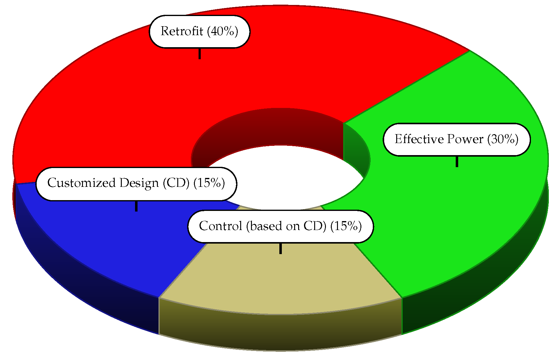
Section 5, the customized approach relying on accurate GIS data was applied. Thanks to this, the power consumption got reduced by approximately 15%. Together with the 15% reduction achieved by the usage of the dynamic control system and 40% reduction related to HID to LED retrofit, we finally obtained about 70% reduction of the power consumed by the considered street lighting installations (
Figure 5).


