Abstract
Cooling towers discharge waste heat from an industrial process into the atmosphere, and are essential for the functioning of large energy-producing plants, including nuclear reactors. Using a numerical simulation model of the cooling tower together with measurements of outlet air relative humidity, outlet air and water temperatures enables the quantification of the rate of thermal energy dissipation removed from the respective process. The computed quantities depend on many model parameters including correlations, boundary conditions, material properties, etc. Changes in these model parameters will induce changes in the computed quantities of interest (called “model responses”). These changes are quantified by the functional derivatives (called “sensitivities”) of the model responses with respect to the model parameters. These sensitivities are computed in this work by applying the general Adjoint Sensitivity Analysis Methodology (ASAM) for nonlinear systems. These sensitivities are needed for: (i) ranking the parameters in their importance to contributing to response uncertainties; (ii) propagating the uncertainties (covariances) in these model parameters to quantify the uncertainties (covariances) in the model responses; (iii) performing predictive modeling, including assimilation of experimental measurements and calibration of model parameters to produce optimal predicted quantities (both model parameters and responses) with reduced predicted uncertainties.
1. Introduction
A mechanical draft cooling tower (MDCT) discharges waste heat from an industrial process into the atmosphere. Cooling towers are essential for the functioning of large energy-producing plants, including nuclear reactors. Using a numerical simulation model of the cooling tower together with measurements of outlet air relative humidity, outlet air and water temperatures enables the quantification of the rate of thermal energy dissipation removed from the respective process. In addition to computing the temperature drop of the cooling water as it passes through the tower, a cooling tower model that derives heat dissipation rates from thermal imagery needs to convert the remotely measured cooling tower throat or area-weighted temperature to a cooling water inlet temperature. Therefore, a cooling tower model comprises two main components, namely: (i) an inner model which computes the amount of cooling undergone by the water as it passes through the tower as a function of inlet cooling water temperature and ambient weather conditions (air temperature and humidity); and (ii) an outer model which uses a remotely measured throat or area-weighted temperature and iterates on the inlet water temperature to match the target temperature of interest. The cooling tower model produces an estimate of the rate at which energy is being discharged to the atmosphere by evaporation and sensible heat transfer. The sensible heat transfer is estimated using the computed change in air or water enthalpy as it passes through the MDCT. If the MDCT fans are on, a prescribed mass flow rate of air and water is used. If the MDCT fans are off, an additional mechanical energy equation is iteratively solved to determine the mass flow rate of air.
The flow regime in the fill section of a cooling tower, which can be cross-flow or counter-flow, determines the type of the respective cooling tower. A model for computing the steady-state thermal performance has been recently presented [1]; this model simulates both cross-flow and counter-flow wet mechanical draft cooling towers. Using as inputs the temperature and mass flow rate of the incoming water together with the temperature and humidity ratio of the incoming ambient air, this model computes the temperature and mass flow rate of the effluent water, as well as the temperature and water vapor content of the exhaust air. The air mass flow rate is specified when the cooling tower operates in the mechanical draft mode. When the fan is turned-off, the cooling tower operates in the natural draft/wind-aided mode, in which case the air mass flow rate is calculated using the numerical model.
In the present work, the counter-flow cooling tower presented in [1] is further developed by applying a considerably more accurate and efficient numerical method for computing the steady state distributions of the following quantities: (i) the water mass flow rates at the exit of each control volume along the height of the fill section of the cooling tower; (ii) the water temperatures at the exit of each control volume along the height of the fill section of the cooling tower; (iii) the air temperatures at the exit of each control volume along the height of the fill section of the cooling tower; (iv) the humidity ratios at the exit of each control volume along the height of the fill section of the cooling tower; and (v) the air relative humidity at the exit of each control volume. In contrast to many cases of non-convergence experienced by the original method [1], the numerical method applied in this work is highly efficient and yields accurate results everywhere, as shown in Section 2.1, below.
More importantly, however, this work presents the development of the adjoint cooling tower sensitivity model for computing efficiently and exactly the sensitivities (i.e., functional derivatives) of the model responses (i.e., quantities of interest) to all 52 model parameters. The adjoint sensitivity model is developed by applying the general Adjoint Sensitivity Analysis Methodology (ASAM) for nonlinear systems, which was originally presented in [2,3,4]. Even though the forward cooling tower model is nonlinear in the state functions, the adjoint sensitivity model is linear in the adjoint state functions, which correspond one-to-one to the forward state functions mentioned in the foregoing. Using the adjoint state functions, the sensitivities of each model response to all of the 52 model parameters can be computed exactly using a single adjoint model computation, as opposed to 52 computations, as would be required if the sensitivities would have been computed—approximately as opposed to exactly—using the forward model in conjunction with finite-differences. The sensitivities are needed for (i) ranking the parameters in the order of their importance for contributing to response uncertainties; (ii) propagating the uncertainties (variances and covariances) in the model parameters to quantify the uncertainties (variances and covariances) in the model responses; (iii) performing predictive modeling, which includes assimilation of experimental measurements and calibration of model parameters to produce optimally predicted nominal values for both model parameters and responses, with reduced predicted uncertainties. The development of the adjoint sensitivity model for the counter-flow cooling tower is presented in Section 2 of this work, together with results for the respective adjoint state functions. A discussion of the significance of the results obtained in this work is presented in Section 3. The predictive modeling of the counter-flow cooling tower will be performed by applying the “predictive modeling for coupled multi-physics systems” (PM_CMPS) methodology recently developed in [5]; the results of this predictive modeling will presented in the sequel to this paper [6].
2. Results
During the period from April, 2004 through August, 2004, a total 8079 measured benchmark data sets for F-area cooling towers (fan-on case) were recorded every fifteen minutes at SRNL for F-Area Cooling Towers [7]. Each of these data sets contained measurements of the following (four) quantities: (i) outlet air temperature measured with the sensor called “Tidbit”, which will be denoted as Ta,out(Tidbit); (ii) outlet air temperature measured with the sensor called “Hobo”, which will be denoted as Ta,out(Hobo); (iii) outlet water temperature, which will be denoted as ; (iv) outlet air relative humidity, which will be denoted as RHmeas. Histogram plots of these 7668 measurement sets (each set containing measurements of Ta,out(Tidbit), Ta,out(Hobo), and RHmeas), together with statistical analyses of these measurements, are presented in Appendix A. These measured quantities provide the basis for the choosing the state functions underlying the mathematical modeling of the cooling tower, which is presented in Section 2.1. An accurate and efficient numerical method for solving the equations underlying the counter-flow cooling tower is also presented in this section. Section 2.2 presents the development of the cooling tower adjoint sensitivity model, along with the solution method for computing the adjoint state functions. The numerical accuracy of solving the equations underlying the adjoint sensitivity model will also be verified.
2.1. Mathematical Model of the Counter-Flow Cooling Tower
The counter-flow cooling tower considered in this work has been originally developed in [1] and is schematically presented in Figure 1.

Figure 1.
Flow through a counter-flow cooling tower.
As this figure indicates, forced air flow enters the tower through the “rain section” above the water basin, flows upward through the fill section and the drift eliminator, and exits at the tower’s top through an exhaust that encloses a fan. Hot water enters above the fill section and is sprayed onto the top of the fill section to create a uniform, downward falling, film flow through the fill’s numerous meandering vertical passages. Film fills are designed to maximize the water free surface area and the residence time inside of the fill section. Heat and mass transfer occurs at the falling film’s free surface between the water film and the upward air flow. The drift eliminator above the spray zone removes entrained water droplets from the upward flowing air. Below the fill section, the water droplets fall into a collection basin, placed at the bottom of the cooling tower. The heat and mass transfer processes occur overwhelmingly in the fill section. Modeling the heat and mass transfer processes between falling water film and rising air in the cooling tower’s fill section is accomplished by solving the following balance equations: (A) liquid continuity; (B) liquid energy balance; (C) water vapor continuity; (D) air/water vapor energy balance. The assumptions used in deriving these equations are as follows:
- the air and/or water temperatures are uniform throughout each stream at any cross section;
- the cooling tower has uniform cross-sectional area;
- the heat and mass transfer occur solely in the direction normal to flows;
- the heat and mass transfer through tower walls to the environment is negligible;
- the heat transfer from the cooling tower fan and motor assembly to the air is negligible;
- the air and water vapor mix as ideal gasses;
- the flow between flat plates is unsaturated through the fill section.
This work considers moderately sized towers for which the heat and mass transfer processes in the rain section is negligible. The fill section is modeled by discretizing it in vertically stacked control volumes as depicted in Figure 2. The heat and mass transfer between the falling water film and the rising air in a typical control volume of the cooling tower’s fill section is presented in Figure 3.
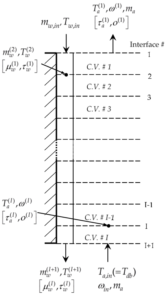
Figure 2.
Control volumes comprising the counter-flow cooling tower, together with the symbols denoting the forward state functions and the adjoint state functions , respectively.
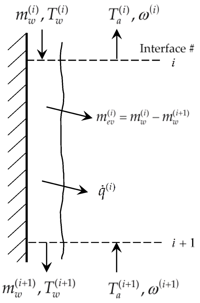
Figure 3.
Heat and mass transfer between falling water film and rising air in a typical control volume of the cooling tower’s fill section.
In the mechanical draft mode, the mass flow rate of dry air is specified. With the fan off and hot water flowing through the cooling tower, air will continue to flow through the tower due to buoyancy. Wind pressure at the air inlet to the cooling tower will also enhance air flow through the tower. The air flow rate is determined from the overall mechanical energy equation for the dry air flow. The state functions underlying the cooling tower model (cf., Figure 1, Figure 2 and Figure 3) are as follows:
- the water mass flow rates, denoted as , at the exit of each control volume, i, along the height of the fill section of the cooling tower;
- the water temperatures, denoted as , at the exit of each control volume, i, along the height of the fill section of the cooling tower;
- the air temperatures, denoted as , at the exit of each control volume, i, along the height of the fill section of the cooling tower; and
- the humidity ratios, denoted as ., at the exit of each control volume, i, along the height of the fill section of the cooling tower.
It is convenient to consider the above state functions to be components of the following (column) vectors:
In this work, the dagger will be used to denote “transposition”, and all vectors will be considered to be column vectors. The governing conservation equations within the total of I = 49 control volumes represented in Figure 2 are as follows [1]:
- Liquid continuity equations:
- (i)
- Control Volume i = 1:
- (ii)
- Control Volumes i = 2,..., I−1:
- (iii)
- Control Volume i = I:
- Liquid energy balance equations:
- (i)
- Control Volume i = 1:
- (ii)
- Control Volumes i = 2,…, I−1:
- (iii)
- Control Volume i = I:
- Water vapor continuity equations:
- (i)
- Control Volume i = 1:
- (ii)
- Control Volumes i = 2,..., I−1:
- (iii)
- Control Volume i = I:
- The air/water vapor energy balance equations:
- (i)
- Control Volume i = 1:
- (ii)
- Control Volumes i = 2,..., I−1:
- (iii)
- Control Volume i = I:
The components of the vector , which appears in Equations (2)–(13), comprise the model parameters which are generically denoted as , i.e.:
where denotes the total number of model parameters. These model parameters are experimentally derived quantities, and their complete distributions parameters are not known; however, we have determined the first four moments (means, variance/covariance, skewness, and kurtosis) of each of these parameter distributions, as detailed in Appendix B.
In the original work [1], the above equations were solved using a two stage-iterative method comprising an “inner-iteration” using Newton’s method within each control volume, followed by an outer iteration aimed at achieving overall convergence. This procedure, though, did not converge at all of the points of interest. Therefore, after testing several alternatives provided in [8] and [9], we have replaced the original solution method in [1] by Newton’s method together with the GMRES linear iterative solver for sparse matrices [10] provided in the NSPCG package [9], which turned out to be the most efficient among those we have tested. This GMRES method [10] approximates the exact solution-vector of a linear system by using the Arnoldi iteration to find the approximate solution-vector by minimizing the norm of the residual vector over a Krylov subspace. The specific computational steps are as follows:
with matrix-components defined in Appendix C. As shown in this Appendix, the Jacobian represented by Equation (18) is a non-symmetric sparse matrix of order 196 by 196, with 14 nonzero diagonals. The non-symmetric diagonal storage format is used to store the respective 14 nonzero diagonals, so that the “condensed” Jacobian matrix has dimensions 196 by 14. Since the Jacobian is highly non-symmetric, the cost of the iterations of the GMRES solver grows as O(m2), where m is the iteration number within the GMRES solver. To reduce this computational cost, the GMRES solver is configured to run with the restart feature. The optimized value for the restart frequency is 10 for this specific application. The MIC preconditioner can speed up the convergence of the GMRES solver using the parameters OMEGA and LVFILL [9] in the modified incomplete factorization methods for the MIC preconditioner; for this application the following values were found to be optimal: OMEGA = 0.000000001 and LVFILL = 1. The Jacobian is not updated inside the sparse GMRES solver. The default convergence of GMRES is tested with the following criterion [9]:
where denotes the pseudo-residual at mth-iteration of the GMRES solver, is the solution of Equation (17) at mth-iteration, and denotes the stopping test value for the GMRES solver.
- (a)
- Write Equations (1)–(13) in vector form as:where the following definitions were used:
- (b)
- Set the initial guess, , to be the inlet boundary conditions;
- (c)
- Steps d through g, below, constitute the outer iteration loop; for , iterate over the following steps until convergence:
- (d)
- Inner iteration loop: for use the iterative GMRES linear solver with the Modified Incomplete Cholesky (MIC) preconditioner, with restarts, to solve, until convergence, the following system to compute the vector :
- (e)
- Setwhere is the current outer loop iteration number, and update the Jacobian.
- (f)
- Test for convergence of the outer loop until the error in the solution is less than a specified maximum value. For solving Equations (2)–(13), the following error criterion has been used:
- (g)
- Set and go to step d.
The above solution strategy for solving Equations (2)–(13) converged successfully for all the 8079 benchmark data sets. As described previously, each of these data sets contained measurements of the following quantities: (i) outlet air temperature measured with the sensor called “Tidbit”; (ii) outlet air temperature measured with the sensor called “Hobo”; (iii) outlet water temperature; (iv) outlet air relative humidity. For each of these benchmark data sets, the outer loop iterations described above (i.e., steps c through g) converge in 4 iterations; for each outer loop iteration, the GMRES solver used for solving Equation (17) converges in 12 iterations. The “zero-to-zero” verification of the solution’s accuracy using Equations (2) through (13) gives an error of the order of .
In view of the above-mentioned measurements, the responses of interest for this work are as follows:
- (a)
- the vector of water mass flow rates at the exit of each control volume i, ;
- (b)
- the vector of water temperatures at the exit of each control volume i, ;
- (c)
- the vector of air temperatures at the exit of each control volume i, ;
- (d)
- the vector , having components of the air relative humidity at the exit of each control volume i, .
While the water mass flow rates , the water temperatures , and the air temperatures are obtained directly as the solutions of Equations (2)–(13), the air relative humidity, , is computed for each control volume using the expression:
The bar plots, showing the respective values of the water mass flow rates , the water temperatures , the air temperatures , and the air relative humidity, , at the exit of each control volume, are presented in Figure 4, Figure 5, Figure 6 and Figure 7, below.

Figure 4.
Bar plot of the water mass flow rates , , at the exit of each control volume along the height of the fill section of the cooling tower.
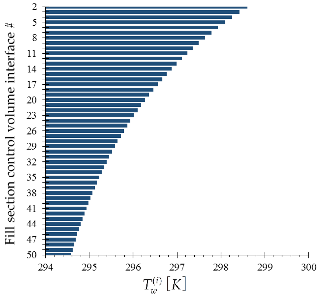
Figure 5.
Bar plot of the water temperatures , , at the exit of each control volume along the height of the fill section of the cooling tower.
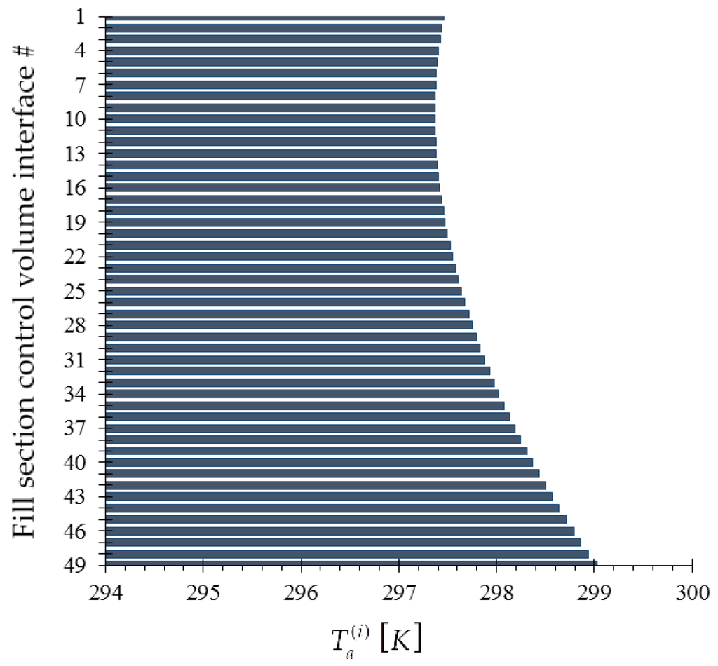
Figure 6.
Bar plot of the air temperatures , , at the exit of each control volume along the height of the fill section of the cooling tower.
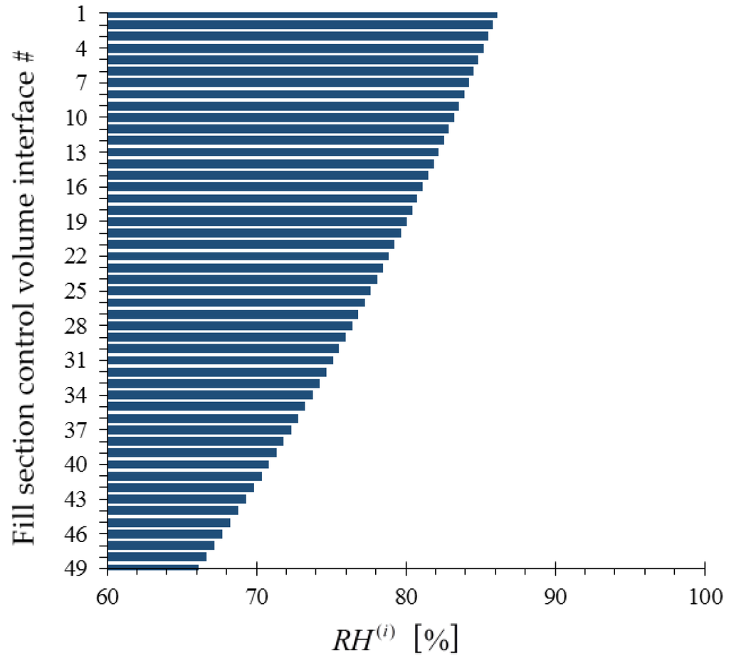
Figure 7.
Bar plot of the air relative humidity , , at the exit of each control volume along the height of the fill section of the cooling tower.
2.2. Development of the Cooling Tower Adjoint Sensitivity Model, with Solution Verification
All of the responses of interest in this work, e.g., the experimentally measured and/or computed responses discussed in the previous Sections, can be generally represented in the functional form , where is a known functional of the model’s state functions and parameters. As generally shown in [2], the sensitivity of such as this response to arbitrary variations in the model’s parameters and state functions is provided by the response’s Gateaux (G-) differential , which is defined as follows:
where the so-called “direct effect” term, , and the so-called “indirect effect” term, , are defined, respectively, as follows:
where the components of the vectors are defined as follows:
Since the model parameters are related to the model’s state functions through Equations (2)–(13), it follows that variations in the model parameter will induce variations in the state variables. More precisely, it has been shown in [2,3,4] that to first-order in the parameter variations, the respective variations in the state variables can be computed by solving the G-differentiated model equations, namely:
Performing the above differentiation on Equations (2) through (13) yields the following forward sensitivity system:
where the components of the vectors are defined as follows:
The system represented by Equation (26) is called the forward sensitivity system, which can be solved, in principle, to compute the variations in the state functions for every variation in the model parameters. In turn, the solution of Equation (26) can be used in Equation (24) to compute the “indirect effect” term, . However, since there are many parameter variations to consider, solving Equation (26) repeatedly to compute becomes computationally impracticable. The need for solving Equation (26) repeatedly to compute can be circumvented by applying the Adjoint Sensitivity Analysis Procedure (ASAM) formulated in [2,3,4]. The ASAM proceeds by forming the inner-product of Equation (26) with a yet unspecified vector of the form , having the same structure as the vector , transposing the resulting scalar equation and using Equation (24). Furthermore, by requiring that the vector satisfy the following adjoint sensitivity system:
it ultimately results that the “indirect effect” term can be expressed in the form
The system represented by Equation (28) is called the adjoint sensitivity system, which –notably– is independent of parameter variations. Therefore, the adjoint sensitivity system needs to be solved only once, to compute the adjoint functions . In turn, the adjoint functions are used to compute , efficiently and exactly, using Equation (29). As an illustrative example of computing response sensitivities using the adjoint sensitivity system, consider that the model response of interest is the air relative humidity, , in a generic control volume i, as given by Equation (21). For this model response, the “direct effect” term, denoted as , is readily obtained in the form:
where:
On the other hand, the “indirect effect” term, denoted as , is readily obtained in the form:
where:
The units of the adjoint functions can be determined from Equation (29) through dimensional analysis. Specifically, the units for the adjoint functions satisfy the following relation:
where ”[R]” denotes the unit of the response R, while the units for the respective equations are as follows:
Table 1 below lists the units of the adjoint functions for four responses: , , and , respectively, in which, denotes exit air temperature; denotes exit water temperature; denotes exit air relative humidity; and denotes exit water mass flow rate.

Table 1.
Units of the adjoint functions for different responses.
Note that the adjoint sensitivity system represented by Equation (28) is linear in the adjoint state functions, so it can be solved by using numerical methods appropriate for large-scale sparse linear systems. In particular, we solved it by using NSPCG, a “Package for Solving Large Sparse Linear Systems by Various Iterative Methods” [9]; 12 to 18 iterations sufficed for solving the adjoint system within convergence criterion of . The bar plots of the adjoint functions corresponding to the four measured responses of interest, namely: (i) the exit air temperature ; (ii) the outlet (exit) water temperature ; (iii) the exit air humidity ratio ; and (iv) the outlet (exit) water mass flow rate , are presented in Figure 8, Figure 9, Figure 10 and Figure 11.
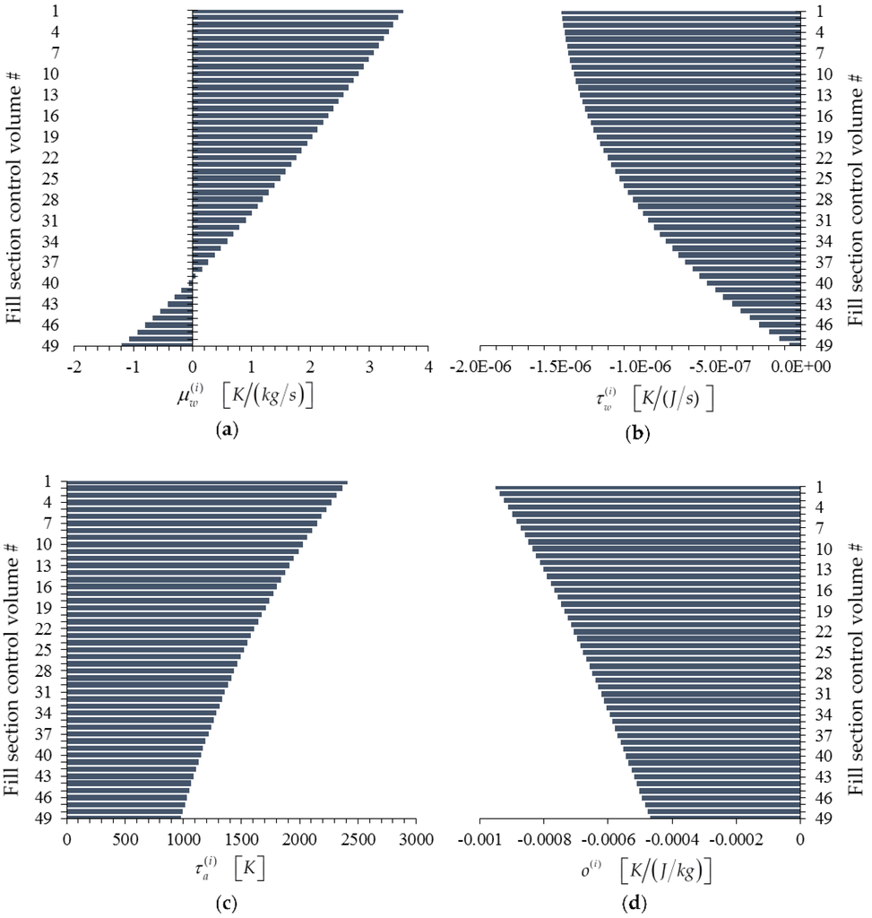
Figure 8.
Bar plots of adjoint functions for the response as functions of the height of the cooling tower’s fill section: (a) ; (b) ; (c) ; (d) .
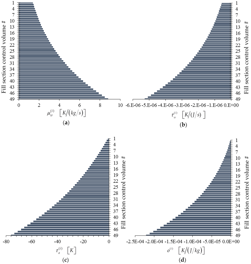
Figure 9.
Bar plots of adjoint functions for the response as functions of the height of the cooling tower’s fill section: (a) ; (b) ; (c) ; (d) .
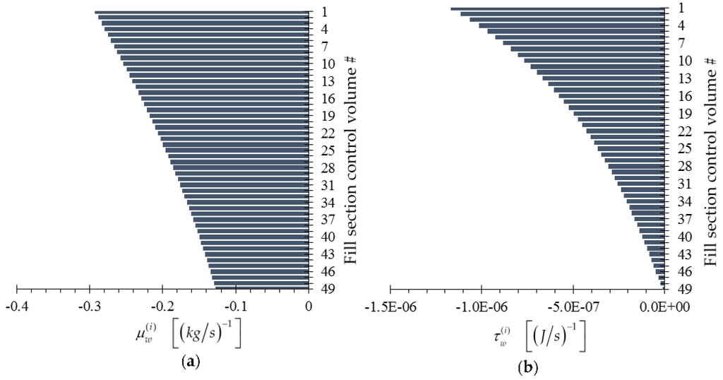

Figure 10.
Bar plots of adjoint functions for the response as functions of the height of the cooling tower’s fill section: (a) ; (b) ; (c) ; (d) .

Figure 11.
Bar plots of adjoint functions for the response , as functions of the height of the cooling tower’s fill section: (a) ; (b) ; (c) ; (d) .
The numerical accuracy of the computed adjoint functions can be independently verified by first noting that Equations (22), (23) and (29) imply that:
where denotes the total number of model parameters, and denotes the “absolute sensitivity” of the response with respect to the parameter , and is defined as:
All of the derivatives with respect to the model parameter on the right side of Equation (40) are known quantities. On the other hand, the absolute response sensitivity can be computed independently, as follows:
- consider a small perturbation in the model parameter ;
- re-compute the perturbed response , where denotes the unperturbed parameter value;
- use the finite difference formula:
- use the approximate equality between Equations (41) and (40) to obtain independently the respective values of the adjoint function(s) being verified.
The verification procedure described in steps (1)–(4) above, will be illustrated in the remainder of this section, for verifying the adjoint functions depicted in Figure 8, Figure 9, Figure 10 and Figure 11.
2.2.1. Verification of the Adjoint Functions for the Outlet Air Temperature Response
When , the quantities defined in Equation (25) all vanish except for a single component, namely: Thus, the adjoint functions corresponding to the outlet air temperature response are computed by solving the adjoint sensitivity system given in Equation (28) using as the only non-zero source term; for this case, the solution of Equation (28) has been depicted in Figure 8.
(a) Verification of the adjoint function
Note that the value of the adjoint function obtained by solving the adjoint sensitivity system given in Equation (28) is , as indicated in Figure 8. Now select a variation in the inlet air temperature , and note that Equation (40) yields the following expression for the sensitivity of the response to :
Re-writing Equation (42) in the form:
indicates that the value of the adjoint function could be computed independently if the sensitivity were available, since the quantity is known. To first-order in the parameter perturbation, the finite-difference formula given in Equation (41) can be used to compute the approximate sensitivity ; subsequently, this value can be used in conjunction with Equation (43) to compute a “finite-difference sensitivity” value, denoted as , for the respective adjoint, which would be accurate up to second-order in the respective parameter perturbation:
Numerically, the inlet air temperature has the nominal (“base-case”) value of . The corresponding nominal value of the response is = 297.4637 . Consider next a perturbation , for which the perturbed value of the inlet air temperature becomes . Re-computing the perturbed response by solving Equations (2)–(13) with the value of yields the “perturbed response” value 297.6073 . Using now the nominal and perturbed response values together with the parameter perturbation in the finite-difference expression given in Equation (41) yields the corresponding “finite-difference-computed sensitivity” . Using this value together with the nominal values of the other quantities appearing in the expression on the right side of Equation (44) yields . This result compares well with the value obtained by solving the adjoint sensitivity system given in Equation (28), cf., Figure 8. When solving this adjoint sensitivity system, the computation of depends on the previously computed adjoint functions ; hence, the forgoing verification of the computational accuracy of also provides an indirect verification that the functions , were also computed accurately.
(b) Verification of the adjoint function
Note that the value of the adjoint function obtained by solving the adjoint sensitivity system given in Equation (28) is , as indicated in Figure 8. Now select a variation in the inlet air humidity ratio , and note that Equation (40) yields the following expression for the sensitivity of the response to :
Re-writing Equation (45) in the form:
indicates that the value of the adjoint function could be computed independently if the sensitivity were available, since the has been verified in (the previous) Section 2.2.1 (a) and the quantity is known. To first-order in the parameter perturbation, the finite-difference formula given in Equation (41) can be used to compute the approximate sensitivity ; subsequently, this value can be used in conjunction with Equation (46) to compute a “finite-difference sensitivity” value, denoted as , for the respective adjoint, which would be accurate up to second-order in the respective parameter perturbation:
Numerically, the inlet air humidity ratio has the nominal (“base-case”) value of . The corresponding nominal value of the response is . Consider next a perturbation , for which the perturbed value of the inlet air humidity ratio becomes . Re-computing the perturbed response by solving Equations (2)–(13) with the value of yields the “perturbed response” value . Using now the nominal and perturbed response values together with the parameter perturbation in the finite-difference expression given in Equation (41) yields the corresponding “finite-difference-computed sensitivity” . Using this value together with the nominal values of the other quantities appearing in the expression on the right side of Equation (47) yields . This result compares well with the value obtained by solving the adjoint sensitivity system given in Equation (28), cf. Figure 8. When solving this adjoint sensitivity system, the computation of depends on the previously computed adjoint functions ; hence, the forgoing verification of the computational accuracy of also provides an indirect verification that the functions were also computed accurately.
(c) Verification of the adjoint functions and
Note that the values of the adjoint functions and obtained by solving the adjoint sensitivity system given in Equation (28) are as follows: and , respectively, as indicated in Figure 8. Now select a variation in the inlet water temperature , and note that Equation (40) yields the following expression for the sensitivity of the response to :
Since the adjoint functions and have been already verified as described in Section 2.2.1 (a) and (b), it follows that the computed values of adjoint functions can also be considered as being accurate, since they constitute the starting point for solving the adjoint sensitivity system in Equation (28). Hence, the unknowns in Equation (48) are the adjoint functions and . A second equation involving solely these adjoint functions can be derived by selecting a perturbation, , in the inlet water mass flow rate, , for which Equation (40) yields the following expression for the sensitivity of the response to :
Numerically, the inlet water temperature, , has the nominal (“base-case”) value of , while the nominal (“base-case”) value of the inlet water mass flow rate is . As before, the corresponding nominal value of the response is . Consider now a perturbation , for which the perturbed value of the inlet air temperature becomes . Re-computing the perturbed response by solving Equations (2)–(13) with the value of yields the “perturbed response” value . Using now the nominal and perturbed response values together with the parameter perturbation in the finite-difference expression given in Equation (41) yields the corresponding “finite-difference-computed sensitivity” .
Next, consider a perturbation , for which the perturbed value of the inlet air temperature becomes . Re-computing the perturbed response by solving Equations (2)–(13) with the value of yields the “perturbed response” value . Using now the nominal and perturbed response values together with the parameter perturbation in the finite-difference expression given in Equation (41) yields the corresponding “finite-difference-computed sensitivity” . Inserting now all of the numerical values of the known quantities in Equations (48) and (49) yields the following system of coupled equations for obtaining and :
Solving Equations (50) and (51) yields and . These values compare well with the values and , respectively, which are obtained by solving the adjoint sensitivity system given in Equation (28), cf. Figure 8.
2.2.2. Verification of the Adjoint Functions for the Outlet Water Temperature Response
When , the quantities defined in Equation (25) all vanish except for a single component, namely: Thus, the adjoint functions corresponding to the outlet water temperature response are computed by solving the adjoint sensitivity system given in Equation (28) using as the only non-zero source term; for this case, the solution of Equation (28) has been depicted in Figure 9.
(a) Verification of the adjoint function
Note that the value of the adjoint function obtained by solving the adjoint sensitivity system given in Equation (28) is , as indicated in Figure 9. Now select a variation in the inlet air temperature , and note that Equation (40) yields the following expression for the sensitivity of the response to :
Re-writing Equation (52) in the form:
indicates that the value of the adjoint function could be computed independently if the sensitivity were available, since the quantity is known. To first-order in the parameter perturbation, the finite-difference formula given in Equation (41) can be used to compute the approximate sensitivity ; subsequently, this value can be used in conjunction with Equation (53) to compute a “finite-difference sensitivity” value, denoted as , for the respective adjoint, which would be accurate up to second-order in the respective parameter perturbation:
Numerically, the inlet air temperature has the nominal (“base-case”) value of . The corresponding nominal value of the response is . Consider next a perturbation , for which the perturbed value of the inlet air temperature becomes . Re-computing the perturbed response by solving Equations (2)–(13) with the value of yields the “perturbed response” value . Using now the nominal and perturbed response values together with the parameter perturbation in the finite-difference expression given in Equation (41) yields the corresponding “finite-difference-computed sensitivity” . Using this value together with the nominal values of the other quantities appearing in the expression on the right side of Equation (54) yields . This result compares well with the value obtained by solving the adjoint sensitivity system given in Equation (28), cf., Figure 9. When solving this adjoint sensitivity system, the computation of depends on the previously computed adjoint functions ; hence, the forgoing verification of the computational accuracy of also provides an indirect verification that the functions were also computed accurately.
(b) Verification of the adjoint function
Note that the value of the adjoint function obtained by solving the adjoint sensitivity system given in Equation (28) is , as indicated in Figure 9. Now select a variation in the inlet air humidity ratio , and note that Equation (40) yields the following expression for the sensitivity of the response to :
Re-writing Equation (55) in the form
indicates that the value of the adjoint function could be computed independently if the sensitivity were available, since the has been verified in (the previous) Section 2.2.2 (a) and the quantity is known. To first-order in the parameter perturbation, the finite-difference formula given in Equation (41) can be used to compute the approximate sensitivity ; subsequently, this value can be used in conjunction with Equation (56) to compute a “finite-difference sensitivity” value, denoted as , for the respective adjoint, which would be accurate up to second-order in the respective parameter perturbation:
Numerically, the inlet air humidity ratio has the nominal (“base-case”) value of . The corresponding nominal value of the response is . Consider next a perturbation , for which the perturbed value of the inlet air humidity ratio becomes . Re-computing the perturbed response by solving Equations (2)–(13) with the value of yields the “perturbed response” value . Using now the nominal and perturbed response values together with the parameter perturbation in the finite-difference expression given in Equation (41) yields the corresponding “finite-difference-computed sensitivity” . Using this value together with the nominal values of the other quantities appearing in the expression on the right side of Equation (57) yields . This result compares well with the value obtained by solving the adjoint sensitivity system given in Equation (28), cf. Figure 9. When solving this adjoint sensitivity system, the computation of depends on the previously computed adjoint functions ; hence, the forgoing verification of the computational accuracy of also provides an indirect verification that the functions were also computed accurately.
(c) Verification of the adjoint functions and
Note that the values of the adjoint functions and obtained by solving the adjoint sensitivity system given in Equation (28) are as follows: and , respectively, as indicated in Figure 9. Now select a variation in the inlet water temperature , and note that Equation (40) yields the following expression for the sensitivity of the response to :
Since the adjoint functions and have been already verified as described in Section 2.2.2 (a) and (b), it follows that the computed values of adjoint functions can also be considered as being accurate, since they constitute the starting point for solving the adjoint sensitivity system in Equation (28). Hence, the unknowns in Equation (58) are the adjoint functions and . A second equation involving solely these adjoint functions can be derived by selecting a perturbation, , in the inlet water mass flow rate, , for which Equation (40) yields the following expression for the sensitivity of the response to :
Numerically, the inlet water temperature, , has the nominal (“base-case”) value of , while the nominal (“base-case”) value of the inlet water mass flow rate is . As before, the corresponding nominal value of the response is . Consider now a perturbation , for which the perturbed value of the inlet air temperature becomes . Re-computing the perturbed response by solving Equations (2)–(13) with the value of yields the “perturbed response” value . Using now the nominal and perturbed response values together with the parameter perturbation in the finite-difference expression given in Equation (41) yields the corresponding “finite-difference-computed sensitivity” .
Next, consider a perturbation , for which the perturbed value of the inlet air temperature becomes . Re-computing the perturbed response by solving Equations (2)–(13) with the value of yields the “perturbed response” value . Using now the nominal and perturbed response values together with the parameter perturbation in the finite-difference expression given in Equation (41) yields the corresponding “finite-difference-computed sensitivity” . Inserting now all of the numerical values of the known quantities in Equations (58) and (59) yields the following system of coupled equations for obtaining and :
Solving Equations (60) and (61) yields and . These values compare well with the values and , respectively, which are obtained by solving the adjoint sensitivity system given in Equation (28), cf. Figure 9.
2.2.3. Verification of the Adjoint Functions for the Outlet Air Relative Humidity Response
When , the quantities defined in Equation (25) all vanish except for two components, namely:
Thus, the adjoint functions corresponding to the outlet air relative humidity response are computed by solving the adjoint sensitivity system given in Equation (28) using and as the only two non-zero source terms; for this case, the solution of Equation (28) has been depicted in Figure 10.
(a) Verification of the adjoint function
Note that the value of the adjoint function obtained by solving the adjoint sensitivity system given in Equation (28) is , as indicated in Figure 10. Now select a variation in the inlet air temperature , and note that Equation (40) yields the following expression for the sensitivity of the response to :
Re-writing Equation (64) in the form:
indicates that the value of the adjoint function could be computed independently if the sensitivity were available, since the quantity is known. To first-order in the parameter perturbation, the finite-difference formula given in Equation (41) can be used to compute the approximate sensitivity ; subsequently, this value can be used in conjunction with Equation (65) to compute a “finite-difference sensitivity” value, denoted as , for the respective adjoint, which would be accurate up to second-order in the parameter perturbation:
Numerically, the inlet air temperature has the nominal (“base-case”) value of . The corresponding nominal value of the response is . Consider next a perturbation , for which the perturbed value of the inlet air temperature becomes . Re-computing the perturbed response by solving Equations (2)–(13) with the value of yields the “perturbed response” value . Using now the nominal and perturbed response values together with the parameter perturbation in the finite-difference expression given in Equation (41) yields the corresponding “finite-difference-computed sensitivity” . Using this value together with the nominal values of the other quantities appearing in the expression on the right side of Equation (66) yields . This result compares well with the value obtained by solving the adjoint sensitivity system given in Equation (28), cf., Figure 10. When solving this adjoint sensitivity system, the computation of depends on the previously computed adjoint functions ; hence, the forgoing verification of the computational accuracy of also provides an indirect verification that the functions were also computed accurately.
(b) Verification of the adjoint function
Note that the value of the adjoint function obtained by solving the adjoint sensitivity system given in Equation (28) is , as indicated in Figure 10. Now select a variation in the inlet air humidity ratio , and note that Equation (40) yields the following expression for the sensitivity of the response to :
Re-writing Equation (67) in the form
indicates that the value of the adjoint function could be computed independently if the sensitivity were available, since the has been verified in (the previous) Section 2.2.3 (a) and the quantity is known. To first-order in the parameter perturbation, the finite-difference formula given in Equation (41) can be used to compute the approximate sensitivity ; subsequently, this value can be used in conjunction with Equation (68) to compute a “finite-difference sensitivity” value, denoted as , for the respective adjoint, which would be accurate up to second-order in the parameter perturbation:
Numerically, the inlet air humidity ratio has the nominal (“base-case”) value of . The corresponding nominal value of the response is . Consider next a perturbation , for which the perturbed value of the inlet air humidity ratio becomes . Re-computing the perturbed response by solving Equations (2)–(13) with the value of yields the “perturbed response” value . Using now the nominal and perturbed response values together with the parameter perturbation in the finite-difference expression given in Equation (41) yields the corresponding “finite-difference-computed sensitivity” . Using this value together with the nominal values of the other quantities appearing in the expression on the right side of Equation (69) yields . This result compares well with the value obtained by solving the adjoint sensitivity system given in Equation (28), cf. Figure 10. When solving this adjoint sensitivity system, the computation of depends on the previously computed adjoint functions ; hence, the forgoing verification of the computational accuracy of also provides an indirect verification that the functions were also computed accurately.
(c) Verification of the adjoint functions and
Note that the values of the adjoint functions and obtained by solving the adjoint sensitivity system given in Equation (28) are as follows: and , respectively, as indicated in Figure 10. Now select a variation in the inlet water temperature , and note that Equation (40) yields the following expression for the sensitivity of the response to :
Since the adjoint functions and have been already verified as described in Section 2.2.3 (a) and (b), it follows that the computed values of adjoint functions and can also be considered as being accurate, since they constitute the starting point for solving the adjoint sensitivity system in Equation (28). Hence, the unknowns in Equation (70) are the adjoint functions and . A second equation involving solely these adjoint functions can be derived by selecting a perturbation, , in the inlet water mass flow rate, , for which Equation (40) yields the following expression for the sensitivity of the response to :
Numerically, the inlet water temperature, , has the nominal (“base-case”) value of , while the nominal (“base-case”) value of the inlet water mass flow rate is . As before, the corresponding nominal value of the response is . Consider now a perturbation , for which the perturbed value of the inlet air temperature becomes . Re-computing the perturbed response by solving Equations (2)–(13) with the value of yields the “perturbed response” value . Using now the nominal and perturbed response values together with the parameter perturbation in the finite-difference expression given in Equation (41) yields the corresponding “finite-difference-computed sensitivity” .
Next, consider a perturbation , for which the perturbed value of the inlet air temperature becomes . Re-computing the perturbed response by solving Equations (2)–(13) with the value of yields the “perturbed response” value . Using now the nominal and perturbed response values together with the parameter perturbation in the finite-difference expression given in Equation (41) yields the corresponding “finite-difference-computed sensitivity” . Inserting now all of the numerical values of the known quantities in Equations (70) and (71) yields the following system of coupled equations for obtaining and :
Solving Equations (72) and (73) yields and . These values compare well with the values and , respectively, which are obtained by solving the adjoint sensitivity system given in Equation (28), cf. Figure 10.
2.2.4. Verification of the Adjoint Functions for the Outlet Water Mass Flow Rate Response
When , the quantities defined in Equation (25) all vanish except for a single component, namely: Thus, the adjoint functions corresponding to the outlet water mass flow rate response are computed by solving the adjoint sensitivity system given in Equation (28) using as the only non-zero source term; for this case, the solution of Equation (28) has been depicted in Figure 11.
(a) Verification of the adjoint function
Note that the value of the adjoint function obtained by solving the adjoint sensitivity system given in Equation (28) is , as indicated in Figure 11. Now select a variation in the inlet air temperature , and note that Equation (40) yields the following expression for the sensitivity of the response to :
Re-writing Equation (74) in the form:
indicates that the value of the adjoint function could be computed independently if the sensitivity were available, since the quantity is known. To first-order in the parameter perturbation, the finite-difference formula given in Equation (41) can be used to compute the approximate sensitivity ; subsequently, this value can be used in conjunction with Equation (75) to compute a “finite-difference sensitivity” value, denoted as , for the respective adjoint, which would be accurate up to second-order in the parameter perturbation:
Numerically, the inlet air temperature has the nominal (“base-case”) value of . The corresponding nominal value of the response is . Consider next a perturbation , for which the perturbed value of the inlet air temperature becomes . Re-computing the perturbed response by solving Equations (2)–(13) with the value of yields the “perturbed response” value . Using now the nominal and perturbed response values together with the parameter perturbation in the finite-difference expression given in Equation (41) yields the corresponding “finite-difference-computed sensitivity” . Using this value together with the nominal values of the other quantities appearing in the expression on the right side of Equation (76) yields . This result compares well with the value obtained by solving the adjoint sensitivity system given in Equation (28), cf., Figure 11. When solving this adjoint sensitivity system, the computation of depends on the previously computed adjoint functions ; hence, the forgoing verification of the computational accuracy of also provides an indirect verification that the functions were also computed accurately.
(b) Verification of the adjoint function
Note that the value of the adjoint function obtained by solving the adjoint sensitivity system given in Equation (28) is , as indicated in Figure 11. Now select a variation in the inlet air humidity ratio , and note that Equation (40) yields the following expression for the sensitivity of the response to :
Re-writing Equation (77) in the form:
indicates that the value of the adjoint function could be computed independently if the sensitivity were available, since the has been verified in (the previous) Section 2.2.4 (a) and the quantity is known. To first-order in the parameter perturbation, the finite-difference formula given in Equation (41) can be used to compute the approximate sensitivity ; subsequently, this value can be used in conjunction with Equation (78) to compute a “finite-difference sensitivity” value, denoted as , for the respective adjoint, which would be accurate up to second-order in the parameter perturbation:
Numerically, the inlet air humidity ratio has the nominal (“base-case”) value of . The corresponding nominal value of the response is . Consider next a perturbation , for which the perturbed value of the inlet air humidity ratio becomes . Re-computing the perturbed response by solving Equations (2)–(13) with the value of yields the “perturbed response” value . Using now the nominal and perturbed response values together with the parameter perturbation in the finite-difference expression given in Equation (41) yields the corresponding “finite-difference-computed sensitivity” . Using this value together with the nominal values of the other quantities appearing in the expression on the right side of Equation (79) yields . This result compares well with the value obtained by solving the adjoint sensitivity system given in Equation (28), cf. Figure 11. When solving this adjoint sensitivity system, the computation of depends on the previously computed adjoint functions ; hence, the forgoing verification of the computational accuracy of also provides an indirect verification that the functions were also computed accurately.
(c) Verification of the adjoint functions and
Note that the values of the adjoint functions and obtained by solving the adjoint sensitivity system given in Equation (28) are as follows: and , respectively, as indicated in Figure 11. Now select a variation in the inlet water temperature , and note that Equation (40) yields the following expression for the sensitivity of the response to :
Since the adjoint functions and have been already verified as described in Section 2.2.4 (a) and (b), it follows that the computed values of adjoint functions can also be considered as being accurate, since they constitute the starting point for solving the adjoint sensitivity system in Equation (28). Hence, the unknowns in Equation (80) are the adjoint functions and . A second equation involving solely these adjoint functions can be derived by selecting a perturbation, , in the inlet water mass flow rate, , for which Equation (40) yields the following expression for the sensitivity of the response to :
Numerically, the inlet water temperature, , has the nominal (“base-case”) value of , while the nominal (“base-case”) value of the inlet water mass flow rate is . As before, the corresponding nominal value of the response is . Consider now a perturbation , for which the perturbed value of the inlet air temperature becomes . Re-computing the perturbed response by solving Equations (2)–(13) with the value of yields the “perturbed response” value . Using now the nominal and perturbed response values together with the parameter perturbation in the finite-difference expression given in Equation (41) yields the corresponding “finite-difference-computed sensitivity” .
Next, consider a perturbation , for which the perturbed value of the inlet air temperature becomes . Re-computing the perturbed response by solving Equations (2)–(13) with the value of yields the “perturbed response” value . Using now the nominal and perturbed response values together with the parameter perturbation in the finite-difference expression given in Equation (41) yields the corresponding “finite-difference-computed sensitivity” . Inserting now all of the numerical values of the known quantities in Equations (80) and (81) yields the following system of coupled equations for obtaining and :
Solving Equations (82) and (83) yields and . These values compare well with the values and , respectively, which are obtained by solving the adjoint sensitivity system given in Equation (28), cf. Figure 11.
3. Discussion
Based on the counter-flow cooling tower presented in [1], this work introduced a considerably more accurate and efficient numerical method for computing the steady state distributions of the following quantities: (i) the water mass flow rates at the exit of each control volume along the height of the fill section of the cooling tower; (ii) the water temperatures at the exit of each control volume along the height of the fill section of the cooling tower; (iii) the air temperatures at the exit of each control volume along the height of the fill section of the cooling tower; (iv) the humidity ratios at the exit of each control volume along the height of the fill section of the cooling tower; and (v) the air relative humidity at the exit of each control volume. Subsequently the adjoint cooling tower sensitivity model was conceived in this work for computing efficiently and exactly the sensitivities (i.e., functional derivatives) of the model responses (i.e., quantities of interest) to all 52 model parameters. The adjoint cooling tower model was developed by applying the general adjoint sensitivity analysis methodology (ASAM) for nonlinear systems, which was originally presented in [2,3,4]. The adjoint sensitivity model is linear in the adjoint state functions, which correspond one-to-one to the forward state functions. Using the adjoint state variables, the sensitivities of each model response to all of the 52 model parameters can be computed exactly using a single adjoint model computation, as opposed to 52 computations, as would be required if the sensitivities had been computed using the forward model in conjunction with approximate finite-differences. The various adjoint state functions were computed and their accuracy was verified, thus setting the stage for the specific numerical computation of the respective response sensitivities. By applying the “predictive modeling for coupled multi-physics systems” (PM_CMPS) methodology recently developed in [5], the sequel to this paper [6] will compute numerically the sensitivities, which will be used for the following purposes (i) ranking the parameters in the order of their importance for contributing to response uncertainties; (ii) propagating the uncertainties (variances and covariances) in the model parameters to quantify the uncertainties (variances and covariances) in the model responses; (iii) performing predictive modeling, which includes assimilation of experimental measurements and calibration of model parameters to produce optimally predicted nominal values for both model parameters and responses, with reduced predicted uncertainties.
Acknowledgments
This work has been partially sponsored by the US Department of Energy (James J. Peltz, Program manager) with the University of South Carolina.
Author Contributions
Dan Cacuci conceived and directed the research reported herein, derived the adjoint sensitivity model, chose the numerical solution methods, and wrote the paper. Dr. Ruixian Fang derived the expressions of the various derivatives with respect to the model parameters, and performed all of the numerical calculations.
Conflicts of Interest
The authors declare no conflict of interest. The founding sponsors had no role in the design of the study; in the collection, analyses, or interpretation of data; in the writing of the manuscript, and in the decision to publish the results.
Appendix A: Statistical Analysis of Experimentally Measured Responses for SRNL F-area Cooling Towers
The Benchmark data sets for F-area cooling tower were compared by SRNL to the results computed using their CTTool code [1] for the air exit relative humility (RH). Based on this comparison, if the computed RH is less than 100%, the corresponding set of measured data is considered to be unsaturated, while if the computed RH is equal to or greater than 100% (super saturation), the corresponding data set is considered to be saturated. Applying this criterion to all of the 8079 benchmark data sets (“fan-on”, with the average exhaust air velocity at the shroud equal to 10 m/s) provided in [7] for F-area cooling towers leads to the identification of 7668 measured data sets that fall into the “unsaturated” case analyzed in this work. Histogram plots of these 7668 measurement sets (each set containing measurements of Ta,out(Tidbit), Ta,out(Hobo), and RHmeas), together with statistical analyses thereof are presented in the remainder of this Appendix.
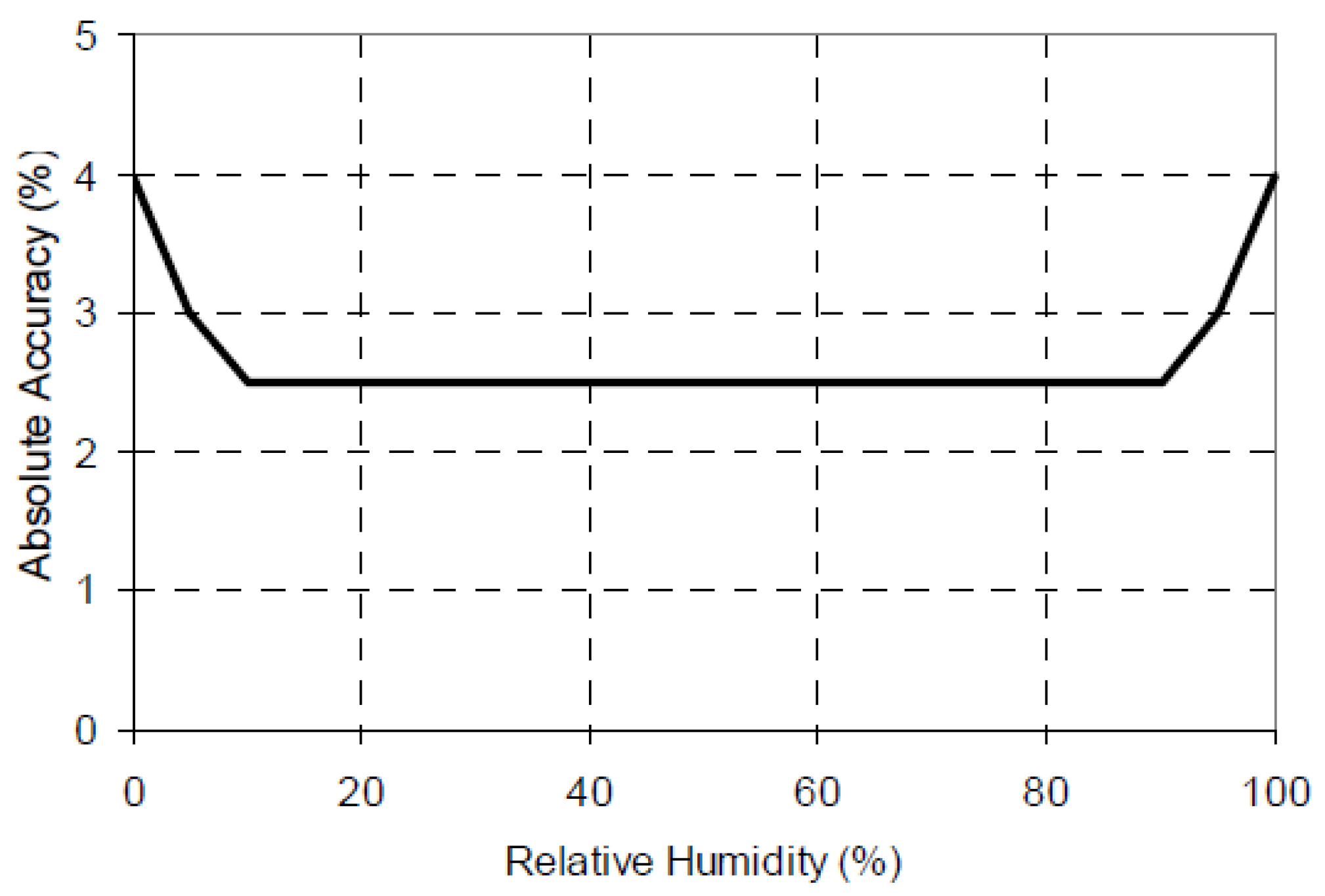
The measured outlet (exit) air relative humidity, RHmeas, was obtained using Hobo humidity sensors. The accuracy of these sensors is depicted in Figure A1, which indicates the following tolerances (standard deviations): ±2.5% for relative humidity from 10% to 90%; between ±2.5% and ±3.5% for relative humidity from 90% to 95%; and ±3.5%~±4.0% from 95% to 100%. However, when exposed to relative humidity above 95%, the maximum sensor error may temporally increase by an additional 1%, so that the error can reach values between ±4.5% to ±5.0% for relative humidity from 95% to 100%.

Figure A1.
Humidity sensor accuracy plot (adopted from the specification of HOBO Pro v2).
Figure A1.
Humidity sensor accuracy plot (adopted from the specification of HOBO Pro v2).
The 7668 measured values of the outlet (exit) air relative humidity, RHmeas , considered according to the results produced by CTTool code [1] to be “unsaturated,” are presented in the histogram plot shown in Figure A2. As shown in this figure, although the computed relative humidity for each of the 7668 data sets is less than 100%, the measured relative humidity RHmeas actually spans the range from 33.0% to 104.1%; in this range, 6975 data sets have their respective RHmeas less than 100% while the other 693 data sets have their respective RHmeas over 100%. This situation is nevertheless consistent with the range of the sensors when their tolerances (standard deviations) are taken into account, which would make it possible for a measurement with RHmeas = 105% to be nevertheless “unsaturated”. Consequently, all the 7668 benchmark data sets plotted in Figure A2 were considered as “unsaturated”, since their respective RHmeas was less than 105%. This plot, as well as all of the other histogram plots in this work, have their total respective areas normalized to unity.
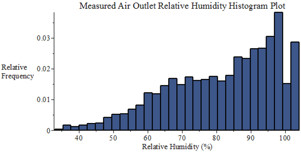
Figure A2.
Histogram plot of the measured air outlet relative humidity, within the 7688 data sets collected by SRNL from F-Area cooling towers (unsaturated conditions).
Figure A2.
Histogram plot of the measured air outlet relative humidity, within the 7688 data sets collected by SRNL from F-Area cooling towers (unsaturated conditions).

The statistical properties of the (measured air outlet relative humidity) distribution shown in Figure A2 have been computed using standard packages, and are presented in Table A1. These statistical properties will be needed for the uncertainty quantification and predictive modeling computations presented in the main body of this work.
Table A1.
Statistics of the air outlet relative humidity distribution [%].
| Minimum | Maximum | Range | Mean | Std. Dev. | Variance | Skewness | Kurtosis |
|---|---|---|---|---|---|---|---|
| 33.0 | 104.1 | 71.1 | 81.98 | 15.63 | 244.44 | −0.60 | 2.55 |
The histogram plots and their corresponding statistical characteristics of the 7668 data sets for the other measurements, namely for: the outlet air temperature [Ta,out(Tidbit)] measured using the “Tidbit” sensors; the outlet air temperature [Ta,out(Hobo)] measured using the “Hobo” sensors; and the outlet water temperature [] are reported below in Figure A3, Figure A4, Figure A5 and Figure A6, and Table A2, Table A3, Table A4 and Table A5, respectively.
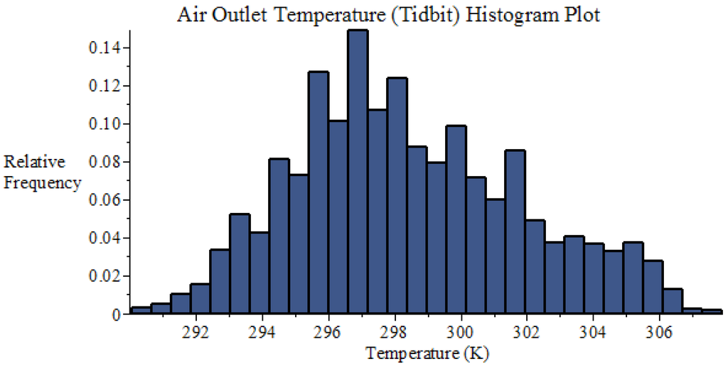
Figure A3.
Histogram plot of the air outlet temperature measured using “Tidbit” sensors, within the 7688 data sets collected by SRNL from F-Area cooling towers (unsaturated conditions).
Figure A3.
Histogram plot of the air outlet temperature measured using “Tidbit” sensors, within the 7688 data sets collected by SRNL from F-Area cooling towers (unsaturated conditions).

Table A2.
Statistics of the air outlet temperature distribution [K], measured using “Tidbit” sensors.
| Minimum | Maximum | Range | Mean | Std. Dev. | Variance | Skewness | Kurtosis |
|---|---|---|---|---|---|---|---|
| 290.06 | 307.89 | 17.83 | 298.42 | 3.42 | 11.71 | 0.34 | 2.52 |

Figure A4.
Histogram plot of the air outlet temperature measured using “Hobo” sensors, within the 7688 data sets collected by SRNL from F-Area cooling towers (unsaturated conditions).
Figure A4.
Histogram plot of the air outlet temperature measured using “Hobo” sensors, within the 7688 data sets collected by SRNL from F-Area cooling towers (unsaturated conditions).
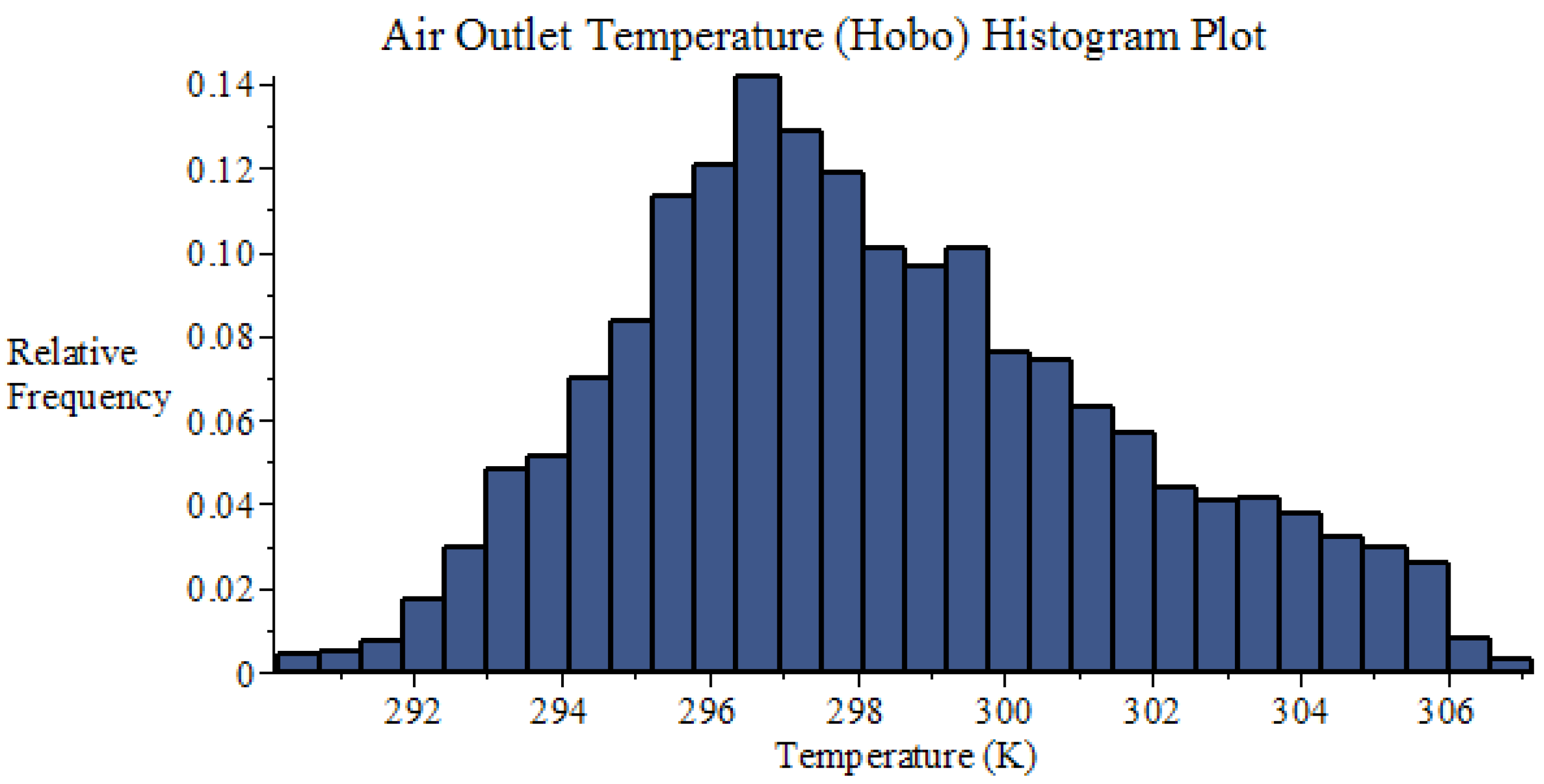
Table A3.
Air outlet temperature distribution statistics [K], measured using “Hobo” sensors.
| Minimum | Maximum | Range | Mean | Std. Dev. | Variance | Skewness | Kurtosis |
|---|---|---|---|---|---|---|---|
| 290.17 | 307.13 | 16.96 | 298.27 | 3.30 | 10.88 | 0.36 | 2.56 |
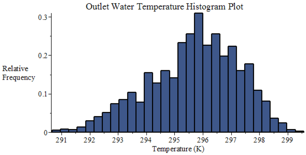
Figure A5.
Histogram plot of water outlet temperature measurements, within the 7688 data sets collected by SRNL from F-Area cooling towers (unsaturated conditions).
Figure A5.
Histogram plot of water outlet temperature measurements, within the 7688 data sets collected by SRNL from F-Area cooling towers (unsaturated conditions).

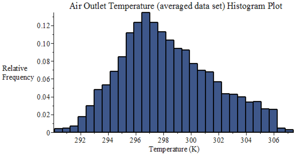
Table A4.
Water outlet temperature distribution statistics [K].
| Minimum | Maximum | Range | Mean | Std. Dev. | Variance | Skewness | Kurtosis |
|---|---|---|---|---|---|---|---|
| 290.67 | 299.57 | 8.90 | 295.68 | 1.58 | 2.48 | −0.41 | 2.72 |
Table A5.
Statistics of the averaged air outlet temperature distribution [K].
| Minimum | Maximum | Range | Mean | Std. Dev. | Variance | Skewness | Kurtosis |
|---|---|---|---|---|---|---|---|
| 290.12 | 307.41 | 17.30 | 298.34 | 3.36 | 11.27 | 0.35 | 2.54 |
Ordering the above-mentioned four measured responses as follows: (i) outlet air temperature Ta,out(Tidbit); (ii) outlet air temperature Ta,out(Hobo); (iii) outlet water temperature ; and (iv) outlet air relative humidity , yields the following “measured response covariance matrix”, denoted as Cov(Ta,out(Tidbit), Ta,out(Hobo), and ):
For the purposes of uncertainty quantification, data assimilation, model calibration and predictive modeling, the temperatures measurements provided by the “Tidbit” and “Hobo” sensors can be combined into an “averaged” data set of measured air outlet temperatures, which will be denoted as . The histogram plot and corresponding statistical characteristics of this averaged air outlet temperature are presented in Figure A6 and Table A5, respectively.
Computing the covariance matrix, denoted as , for all of the relevant experimental data for the averaged outlet air temperature , the outlet water temperature , and the outlet air relative humidity , yields the following result:
Comparing the results in Equations (A1) and (A2) shows that eliminating the second column and row in Equation (A1) yields a 3-by-3 matrix which has entries essentially equivalent to the covariance matrix in Equation (A2). In turn, this result indicates that the temperature distributions measured by the “Tidbit” and “Hobo” sensors, respectively, need not be treated as separate data sets for the purposes of uncertainty quantification and predictive modeling.
The sensors’ standard deviations (namely: for each of the responses and , and for the response ) have been taken into account for the data at the 100%-saturation point, by including the 693 data sets that have their respective measured relative humidity, , between 100% and 104.1%. In addition, the respective sensors’ uncertainties (standard deviations) must also be taken into account for the 6975 data sets that have their respective less than 100%. Since the various measuring methods and devices are independent of each other, the standard deviation, , stemming from the statistical analysis of the 7668 benchmark data sets and the standard deviation, , stemming from the instrument’s uncertainty are to be combined according to the well-known formula “addition of the variances of uncorrelated variates”, namely:
Using the relation in the above Equation (A3) in conjunction with the result presented in Equation (A2) will lead to an increase of the variances on the diagonal of the respective “measured covariance matrix”, which will be denoted as . The final result obtained is:
As indicated in the accompanying PART II [6], the predictive modeling formalism (which includes uncertainty quantification, data assimilation, and model calibration) also requires as “input” the covariance matrix between the measured parameters and responses. All of the parameters and responses are uncorrelated, except possibly for the measured responses considered in this Appendix and the measured parameters considered in Appendix B. The following “parameter-response” covariance matrix, denoted as , is obtained for the respective parameters (namely: dry-bulb air temperature, ; dew-point air temperature, , inlet water temperature, , and atmospheric pressure, ) and responses (i.e., average outlet air temperature, outlet water temperature, and outlet air relative humidity):
Appendix B. Model Parameters for the SRNL F-Area Cooling Towers
The mean values and standard deviations for the independent model parameters presented in Table B1, below, have been derived in collaboration with Dr. Sebastian Aleman of SRNL (private communications, 2016).
Table B1.
Parameters for SRNL F-area Cooling Towers.
| Index i of αi | Independent Scalar Parameters | C++ String | Math. Notation | Nominal Value (s) | Absolute Std. Dev. | Rel. Std. Dev. (%) |
| 1 | Air temperature (dry bulb) (K) | tdb | 299.11 | 4.17 | 1.39 | |
| 2 | Dew point temperature (K) | tdp | 292.05 | 2.36 | 0.81 | |
| 3 | Inlet water temperature (K) | twin | 298.79 | 1.70 | 0.57 | |
| 4 | Atmospheric pressure (Pa) | patm | 100586 | 401 | 0.40 | |
| 5 | Wetted fraction of fill surface area | wtsa | 1 | 0 | 0 | |
| 6 | Sum of loss coefficients above fill | ksum | 10 | 5 | 50 | |
| 7 | Dynamic viscosity of air at T = 300 K (kg/m s) | muair | 1.983E−05 | 9.676E−7 | 4.88 | |
| 8 | Kinematic viscosity of air at T = 300 K (m2/s) | nuair | 1.568E−05 | 1.895E−6 | 12.09 | |
| 9 | Thermal conductivity of air at T = 300 K (W/m K) | tcair | 0.02624 | 1.584E−3 | 6.04 | |
| 10 | Heat transfer coefficient multiplier | mlthtc | 1 | 0.5 | 50 | |
| 11 | Mass transfer coefficient multiplier | mltmtc | 1 | 0.5 | 50 | |
| 12 | Fill section frictional loss multiplier | mltfil | 4 | 2 | 50 | |
| 13 | Pvs(T) parameters | a0 | 25.5943 | 0.01 | 0.04 | |
| 14 | a1 | −5229.89 | 4.4 | 0.08 | ||
| 15 | Cpa(T) parameters | A(1) | 1030.5 | 0.2940 | 0.03 | |
| 16 | A(2) | −0.19975 | 0.0020 | 1.00 | ||
| 17 | A(3) | 3.9734E−04 | 3.345E−6 | 0.84 | ||
| 18 | Dav(T) parameters | A(1) | 7.06085E−9 | 0 | 0 | |
| 19 | A(2) | 2.65322 | 0.003 | 0.11 | ||
| 20 | A(3) | −6.1681E−03 | 2.3E−5 | 0.37 | ||
| 21 | A(4) | 6.55266E−6 | 3.8E−8 | 0.58 | ||
| 22 | hf(T) parameters | a0f | −1143423.78 | 543. | 0.05 | |
| 23 | a1f | 4186.50768 | 1.8 | 0.04 | ||
| 24 | hg(T) parameters | a0g | 2005743.99 | 1046 | 0.05 | |
| 25 | a1g | 1815.437 | 3.5 | 0.19 | ||
| 26 | Nu parameters | - | 8.235 | 2.059 | 25 | |
| 27 | - | 0.00314987 | 0.001 | 31.75 | ||
| 28 | Nu Parameters | - | 0.9902987 | 0.327 | 33.02 | |
| 29 | - | 0.023 | 0.0088 | 38.26 | ||
| 30 | Cooling tower deck width in x-dir. (m) | dkxw | 8.5 | 0.085 | 1 | |
| 31 | Cooling tower deck width in y-dir. (m) | dkyw | 8.5 | 0.085 | 1 | |
| 32 | Cooling tower deck height above ground (m) | dkht | 10 | 0.1 | 1 | |
| 33 | Fan shroud height (m) | fsht | 3.0 | 0.03 | 1 | |
| 34 | Fan shroud inner diameter (m) | fsid | 4.1 | 0.041 | 1 | |
| 35 | Fill section height (m) | flht | 2.013 | 0.02013 | 1 | |
| 36 | Rain section height (m) | rsht | 1.633 | 0.01633 | 1 | |
| 37 | Basin section height (m) | bsht | 1.168 | 0.01168 | 1 | |
| 38 | Drift eliminator thickness (m) | detk | 0.1524 | 0.001524 | 1 | |
| 39 | Fill section equivalent diameter (m) | deqv | 0.0381 | 0.000381 | 1 | |
| 40 | Fill section flow area (m2) | flfa | 67.29 | 6.729 | 10 | |
| 41 | Fill section surface area (m2) | flsa | 14221 | 3555.3 | 25 | |
| 42 | Prandlt number of air at T = 80 C | Pr | 0.708 | 0.005 | 0.71 | |
| 43 | Wind speed (m/s) | wspd | 1.80 | 0.92 | 51.1 | |
| 44 | Exit air speed at the shroud (m/s) | vexit | 10.0 | 1.0 | 10.0 | |
| Index i of αi | Boundary Parameters | C++ String | Math. Notation | Nominal Value | Absolute Std. Dev. | Rel. Std. Dev. (%) |
| 45 | Inlet water mass flow rate (kg/s) | mfwin | 44.02 | 2.201 | 5 | |
| 46 | Inlet air temperature (K) | tain | set to | 4.17 | 1.39 | |
| 47 | Inlet air mass flow rate (kg/s) | main | 155.07 | 15.91 | 10.26 | |
| 48 | Inlet air humidity ratio (Dependent Scalar Parameter) | hrin | 0.0138 | 0.00206 | 14.93 | |
| Index i of αi | Special Dependent Parameters | C++ String | Math. Notation | Nominal Value | Absolute Std. Dev. | Rel. Std. Dev. (%) |
| 49 | Reynold's number | Re; Reh | 4428 | 671.6 | 15.17 | |
| 50 | Schmidt number | Sc | 0.60 | 0.074 | 12.41 | |
| 51 | Sherwood number | Sh | 14.13 | 4.84 | 34.25 | |
| 52 | Nusselt number | Nu | 14.94 | 5.08 | 34.00 |
The above independent model parameters are used for computing various dependent model parameters and thermal material properties, as shown in Table B2 and Table B3, below.
Table B2.
Dependent Scalar Model Parameters.
| Dependent Scalar Parameters | Math. Notation | Defining Equation or Correlation |
|---|---|---|
| Mass diffusivity of water vapor in air (m2/s) | ||
| Heat transfer coefficient (W/m2 K) | ||
| Mass transfer coefficient (m/s) | ||
| Heat transfer term (W/K) | ||
| Mass transfer term (m3/s) | ||
| Density of dry air (kg/m3) | ||
| Air velocity in the fill section (m/s) | ||
| Fill falling-film surface area per vertical section (m2) | ||
| Rain section inlet flow area (m2) | ||
| Height for natural convection (m) | ||
| Height above fill section (m) | ||
| Fill section control volume height (m) | ||
| Fill section length, including drift eliminator (m) | ||
| Fan shroud inner radius (m) | ||
| Fan shroud flow area (m2) |
Table B3.
Thermal Properties (Dependent Scalar Model Parameters).
| Thermal Properties (Functions of State Variables) | Math. Notation | Defining Equation or Correlation |
|---|---|---|
| hf(Tw) = saturated liquid enthalpy (J/kg) | ||
| Hg(Tw) = saturated vapor enthalpy (J/kg) | ||
| Hg(Ta) = saturated vapor enthalpy (J/kg) | ||
| Cp(T) = specific heat of dry air (J/kg K) | ||
| Pvs(Tw) = saturation pressure (Pa) | ||
| Pvs(Ta) = saturation pressure (Pa) |
- Note 1:
- The parameters through (i.e., the dry bulb air temperature, dew point temperature, inlet water temperature, and atmospheric pressure) were measured at the SRNL site at which the F-area cooling towers are located. Among the 8079 measured benchmark data sets [7], 7688 data sets are considered to represent “unsaturated conditions”, which have been used to derive the statistical properties (means, variance and covariance, skewness and kurtosis) for these model parameters, as shown below in Figure B1, Figure B2, Figure B3 and Figure B4 and Table B4, Table B5, Table B6 and Table B7.
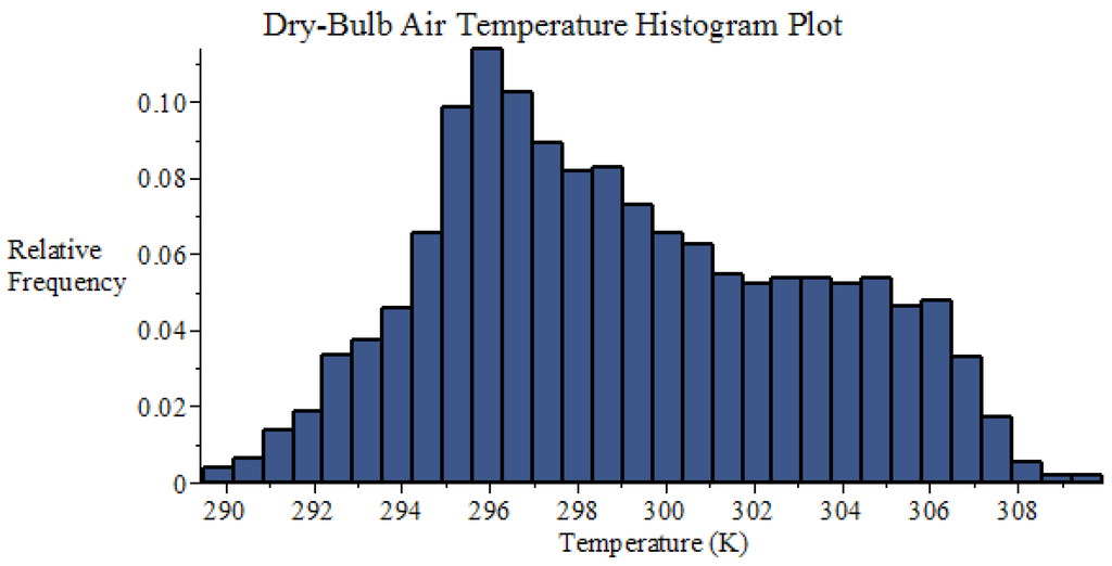
Figure B1.
Histogram plot of dry-bulb air temperature data collected by SRNL from F-Area cooling towers (unsaturated conditions).
Figure B1.
Histogram plot of dry-bulb air temperature data collected by SRNL from F-Area cooling towers (unsaturated conditions).

Table B4.
Statistics of the dry-bulb temperature (set to air inlet temperature) distribution [K].
| Minimum | Maximum | Range | Mean | Std. Dev. | Variance | Skewness | Kurtosis |
|---|---|---|---|---|---|---|---|
| 289.50 | 309.91 | 20.41 | 299.11 | 4.17 | 17.37 | 0.25 | 2.18 |

Figure B2.
Histogram plot of dew-point air temperature data collected by SRNL from F-Area cooling towers (unsaturated conditions).
Figure B2.
Histogram plot of dew-point air temperature data collected by SRNL from F-Area cooling towers (unsaturated conditions).
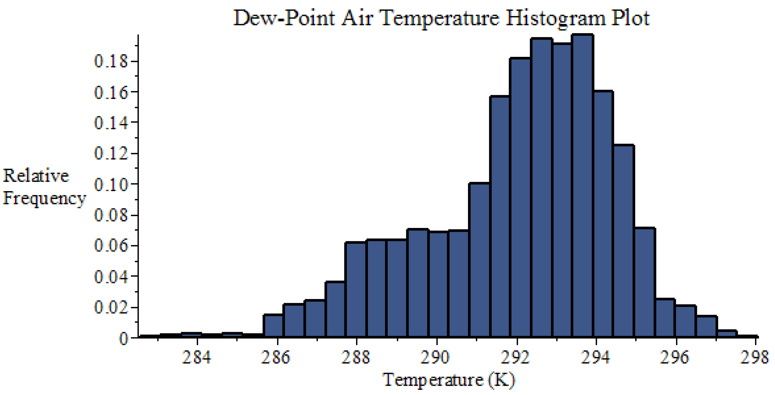
Table B5.
Statistics of the dew-point temperature distribution [K].
| Minimum | Maximum | Range | Mean | Std. Dev. | Variance | Skewness | Kurtosis |
|---|---|---|---|---|---|---|---|
| 282.58 | 298.06 | 15.48 | 292.05 | 2.36 | 5.57 | −0.66 | 3.10 |

Figure B3.
Histogram plot of inlet water temperature data collected by SRNL from F-Area cooling towers (unsaturated conditions).
Figure B3.
Histogram plot of inlet water temperature data collected by SRNL from F-Area cooling towers (unsaturated conditions).

Table B6.
Statistics of the inlet water temperature distribution [K].
| Minimum | Maximum | Range | Mean | Std. Dev. | Variance | Skewness | Kurtosis |
|---|---|---|---|---|---|---|---|
| 293.93 | 303.39 | 9.46 | 298.79 | 1.70 | 2.90 | −0.12 | 2.84 |
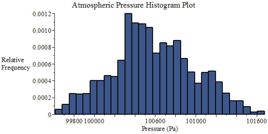
Figure B4.
Histogram plot of atmospheric pressure data collected by SRNL from F-Area cooling towers (unsaturated conditions).
Figure B4.
Histogram plot of atmospheric pressure data collected by SRNL from F-Area cooling towers (unsaturated conditions).

Table B7.
Statistics of the atmospheric pressure distribution [Pa].
| Minimum | Maximum | Range | Mean | Std. Dev. | Variance | Skewness | Kurtosis |
|---|---|---|---|---|---|---|---|
| 99617 | 101677 | 2060 | 100586 | 401 | 160597 | 0.10 | 2.58 |
The 4-by-4 covariance matrix for the above experimental data has also been computed and is provided below, with the four model parameters ordered as follows: dry-bulb air temperature , dew-point air temperature , inlet water temperature , and atmospheric air pressure .
The covariance matrix (above) neglects the uncertainty associated with sensor readings throughout the data collection period. When combining uncertainties by adding variances, the contribution from the sensors is 0.04 K for each of the first three parameters, which accounts for a maximum of ca. 1% of the total variance (for the inlet water temperature, specifically). The uncertainty in the atmospheric pressure sensor is at this time unknown. For these reasons, their contribution to overall uncertainty is considered insignificant at this time.
- Note 2:
- Temperature and pressure values are initially input in units of [C] and [mb], respectively, but are internally converted to [K] and [Pa] for computational purposes.
- Note 3:
- Inlet air humidity ratio is defined as follows:
- Note 4:
- The Reynold’s number is defined (equivalently) as follows:
- Note 5:
- The Schmidt number is defined as follows:
- Note 6:
- The Sherwood number is defined as follows:
- Note 7:
- The Nusselt number is defined as follows:
- Note 8:
- The overall uncertainty of the Nusselt number is estimated to be 25% in the laminar flow region, 40% in the turbulent flow region, and the uncertainty is assumed to increase linearly in the transition region. This is a more conservative estimate of the overall uncertainty than assuming 25% for all three regimes.
- Note 9:
- The inlet water mass flow rate is calculated using the following expression:where:
- Note 10:
- The inlet air mass flow rate is calculated using the following expression:
Appendix C. Derivative Matrix (Jacobian) of the Model Equations with Respect to the State Functions
The functional derivatives of Equations (2) through (13) with respect to the vector-valued state function , where ; ; ; and , will be denoted as follows:
The scope of this Appendix is to provide the specific expressions of each of the above functional derivatives. Derivatives of the liquid continuity equations with respect to the state variables:
The derivatives of the “liquid continuity equations” [cf., Equations (2)–(4)] with respect to are as follows:
For subsequent use, the above quantities are considered to be the components of the matrix defined as follows:
The derivatives of the “liquid continuity equations” [cf. Equations (2)–(4)] with respect to are as follows:
For subsequent use, the above quantities are considered to be the components of the diagonal matrix defined as follows:
The derivatives of the “liquid continuity equations” [cf. Equations (2)–(4)] with respect to are as follows:
For subsequent use, the above quantities are considered to be the components of the diagonal matrix defined as follows:
The derivatives of the “liquid continuity equations” [cf. Equations (2)–(4)] with respect to are as follows:
For subsequent use, the above quantities are considered to be the components of the diagonal matrix defined as follows:
The derivatives of the liquid energy balance equations [cf. Equations (5)–(7)] with respect to are as follows:
For subsequent use, the above quantities are considered to be the components of the matrix defined as follows:
The derivatives of the liquid energy balance equations [cf. Equations (5)–(7)] with respect to are as follows:
For subsequent use, the above quantities are considered to be the components of the diagonal matrix defined as follows:
The derivatives of the liquid energy balance equations [cf. Equations (5)–(7)] with respect to are as follows:
For subsequent use, the above quantities are considered to be the components of the diagonal matrix defined as follows:
The derivatives of the liquid energy balance equations [cf. Equations (5)–(7)] with respect to are as follows:
For subsequent use, the above quantities are considered to be the components of the matrix
The derivatives of the water vapor continuity equations [cf. Equations (8) –(10)] with respect to are as follows:
For subsequent use, the above quantities are considered to be the components of the matrix defined as follows:
The derivatives of the water vapor continuity equations [cf. Equations (8)–(10)] with respect to are as follows:
For subsequent use, the above quantities are considered to be the components of the matrix
The derivatives of the water vapor continuity equations [cf. Equations (8)–(10)] with respect to are as follows:
For subsequent use, the above quantities are considered to be the components of the matrix
The derivatives of the water vapor continuity equations [cf. Equations (8)–(10)] with respect to are as follows:
For subsequent use, the above quantities are considered to be the components of the matrix defined as follows:
The derivatives of the air/water vapor energy balance equations [cf. Equations (11)–(13)] with respect to are as follows:
For subsequent use, the above quantities are considered to be the components of the matrix defined as follows:
The derivatives of the air/water vapor energy balance equations [cf. Equations (11)–(13)] with respect are as follows:
For subsequent use, the above quantities are considered to be the components of the diagonal matrix defined as follows:
The derivatives of the air/water vapor energy balance equations [cf. Equations (11)–(13)] with respect to are as follows:
For subsequent use, the above quantities are considered to be the components of the diagonal matrix defined as follows:
The derivatives of the air/water vapor energy balance equations [cf. Equations (11)–(13)] with respect to are as follows:
For subsequent use, the above quantities are considered to be the components of the diagonal matrix defined as follows:
References
- Aleman, S.E.; Garrett, A.J. Operational Cooling Tower Model (CTTool v1.0); SRNL-STI-2015–00039, Revision 0; Savannah River National Laboratory: Aiken, SC, USA, 2015. [Google Scholar]
- Cacuci, D.G. Sensitivity theory for nonlinear systems: I. Nonlinear functional analysis approach. J. Math. Phys. 1981, 22, 2794–2802. [Google Scholar] [CrossRef]
- Cacuci, D.G. Sensitivity and Uncertainty Analysis: Theory, Volume 1; Chapman & Hall/CRC: Boca Raton, FL, USA, 2003. [Google Scholar]
- Cacuci, D.G.; Ionescu-Bujor, M.; Navon, M.I. Sensitivity and Uncertainty Analysis: Applications to Large Scale Systems, Volume 2; Chapman & Hall/CRC: Boca Raton, FL, USA, 2005. [Google Scholar]
- Cacuci, D.G. Predictive Modeling of Coupled Multi-Physics Systems: I. Theory. Ann. Nucl. Energy 2014, 70, 266–278. [Google Scholar] [CrossRef]
- Fang, R.; Cacuci, D.G.; Badea, M.C. Predictive modelling of a paradigm mechanical cooling tower. II: Optimal best-estimate predictions with reduced uncertainties. Energies 2016. under review. [Google Scholar]
- Garrett, A.J.; Parker, M.J.; Villa-Aleman, E. 2004 Savannah River site Cooling Tower Collection, SRNL-DOD-2005–07; Atmospheric Technologies Group, Savannah River National Laboratory: Aiken, SC, USA, 2005. [Google Scholar]
- Collier, M.; Hindmarsh, A.C.; Serban, R.; Woodward, C.S. User Documentation for KINSOL v2.8.2; Center for Applied Scientific Computing of Lawrence Livermore National Laboratory: Livermore, CA, USA, 2015. [Google Scholar]
- Oppe, T.C.; Joubert, W.D.; Kincaid, D.R. A Package for Solving Large Sparse Linear Systems by Various Iterative Methods, NSPCG User's Guide, Version 1.0; Center for Numerical Analysis, the University of Texas at Austin: Austin, TX, USA, April 1988. [Google Scholar]
- Saad, Y.; Schultz, M.H. GMRES: A generalized minimal residual algorithm for solving nonsymmetric linear systems. SIAM J. Sci. Stat. Comp. 1986, 7, 856–869. [Google Scholar] [CrossRef]
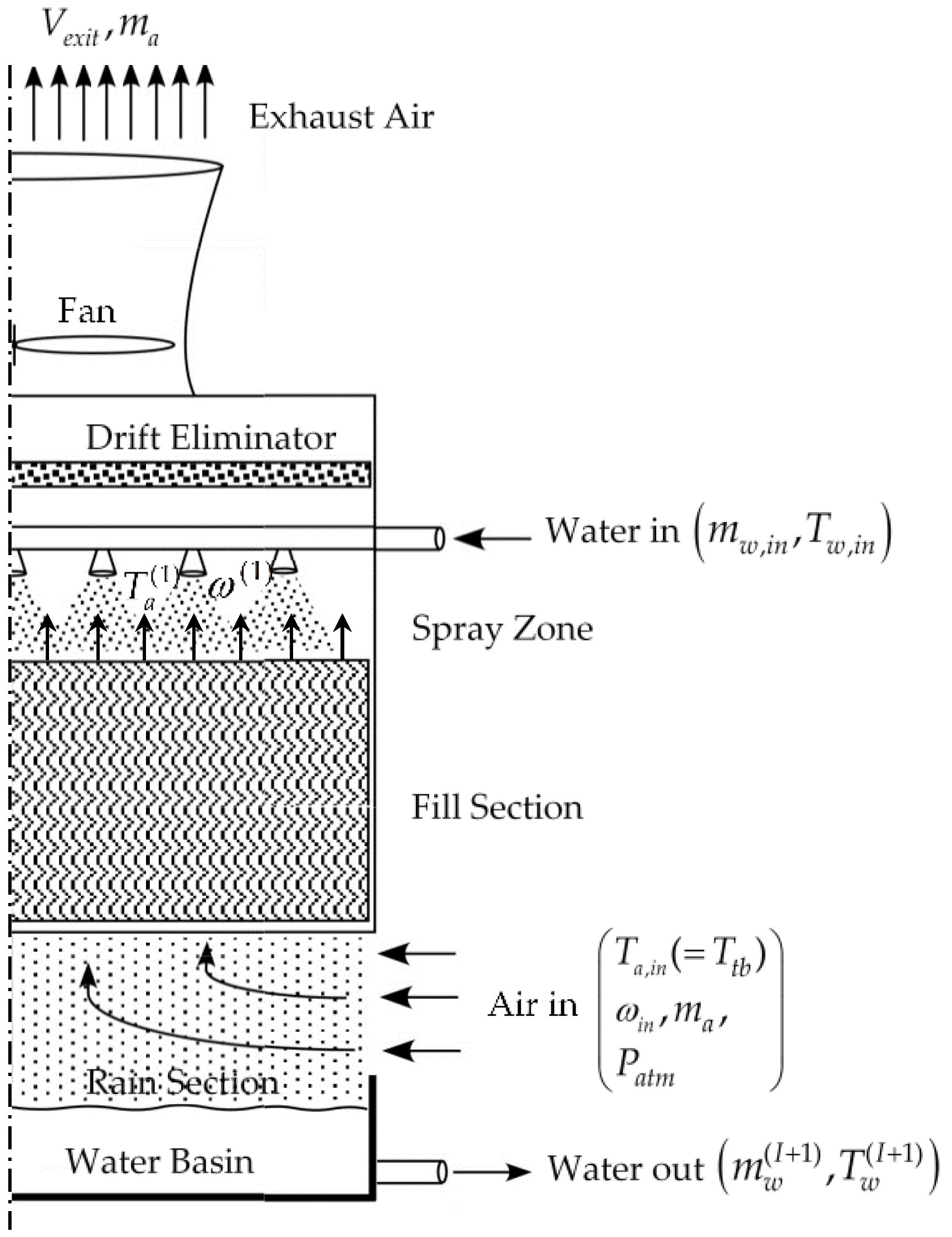

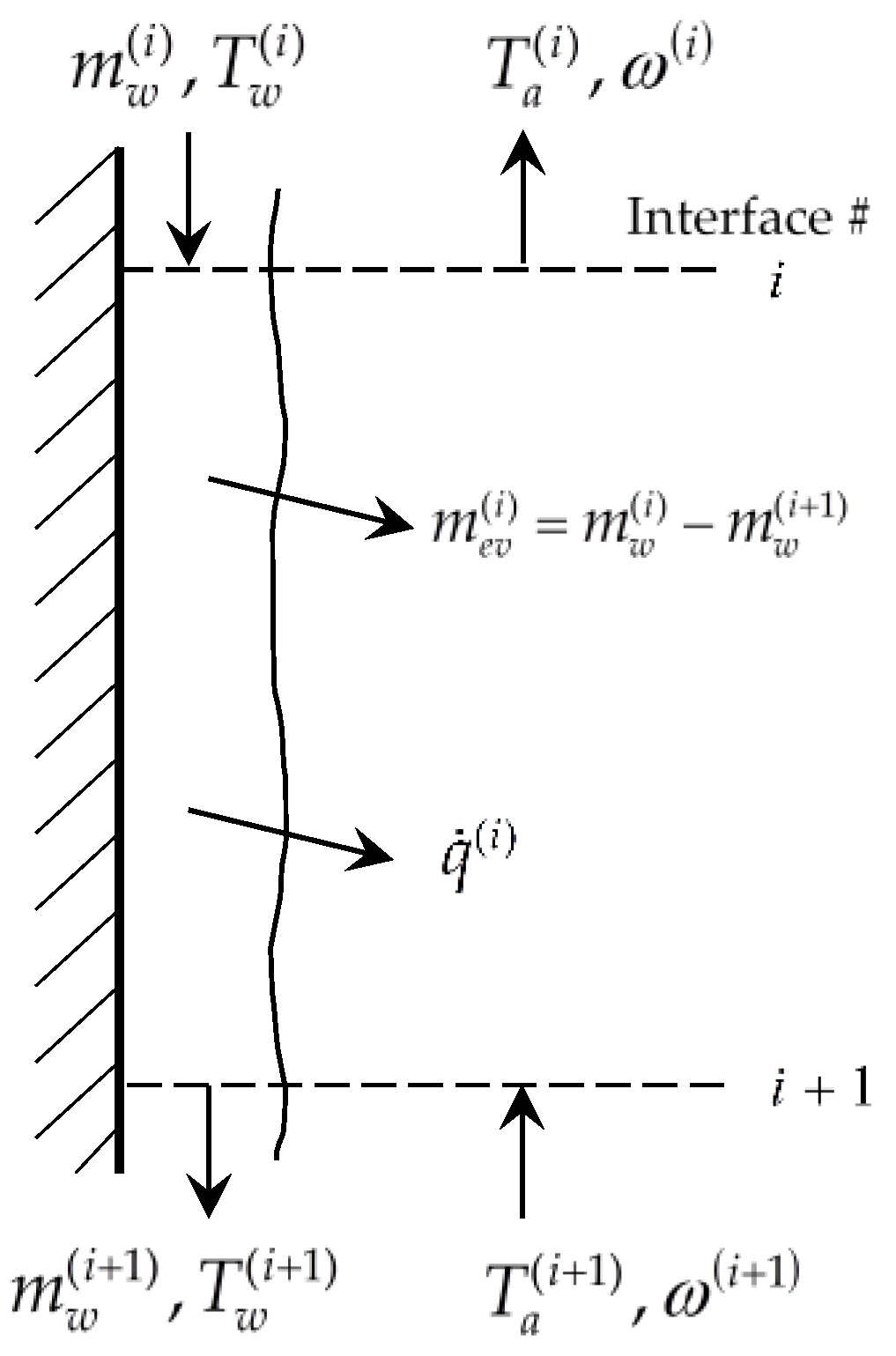
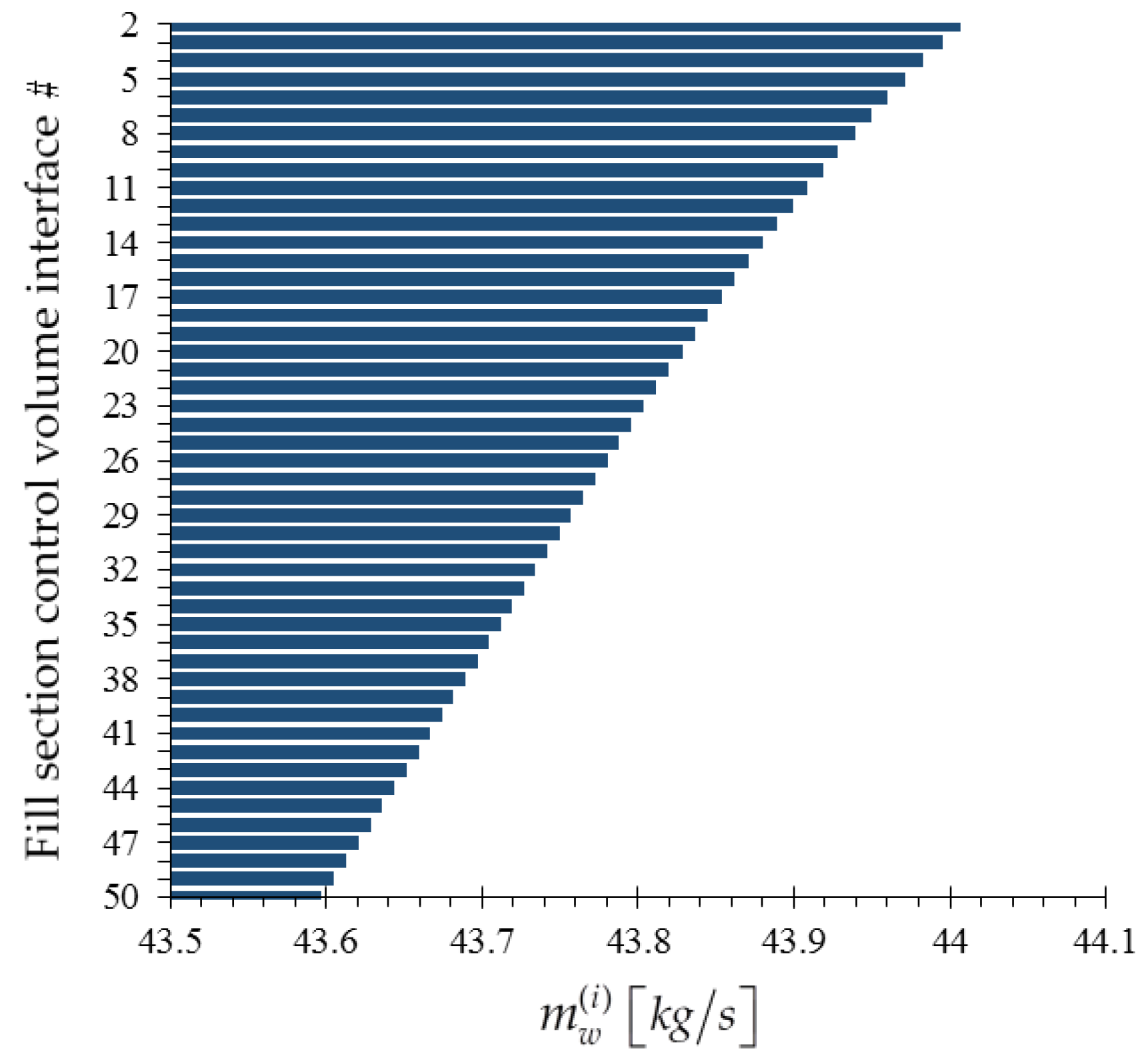


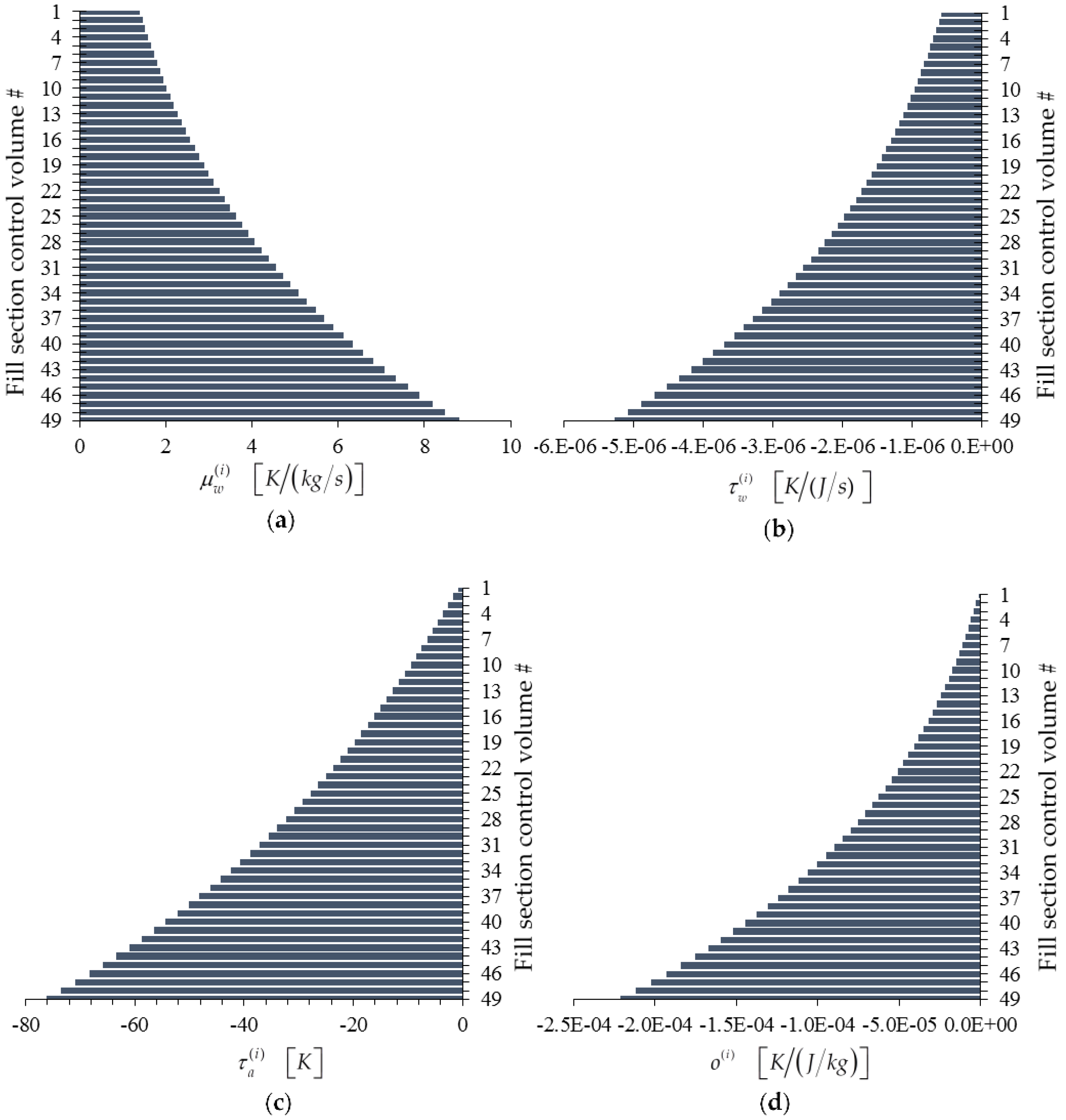

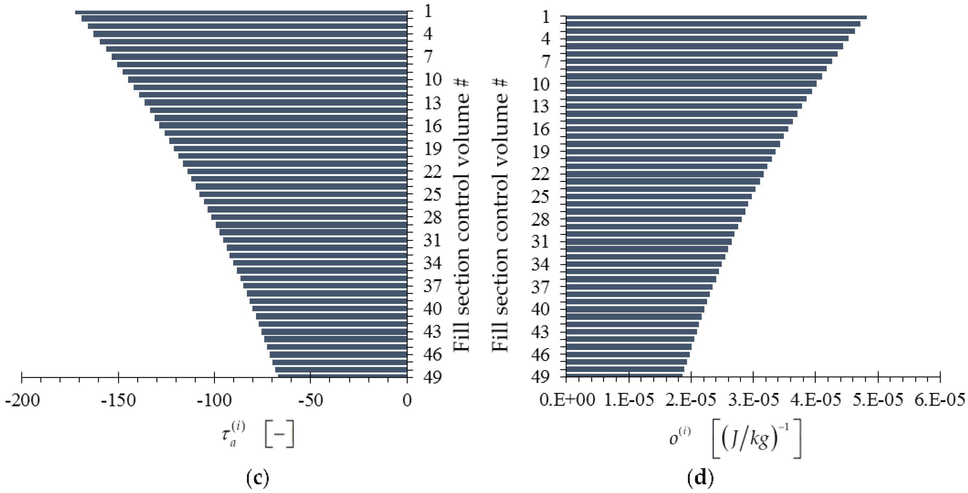
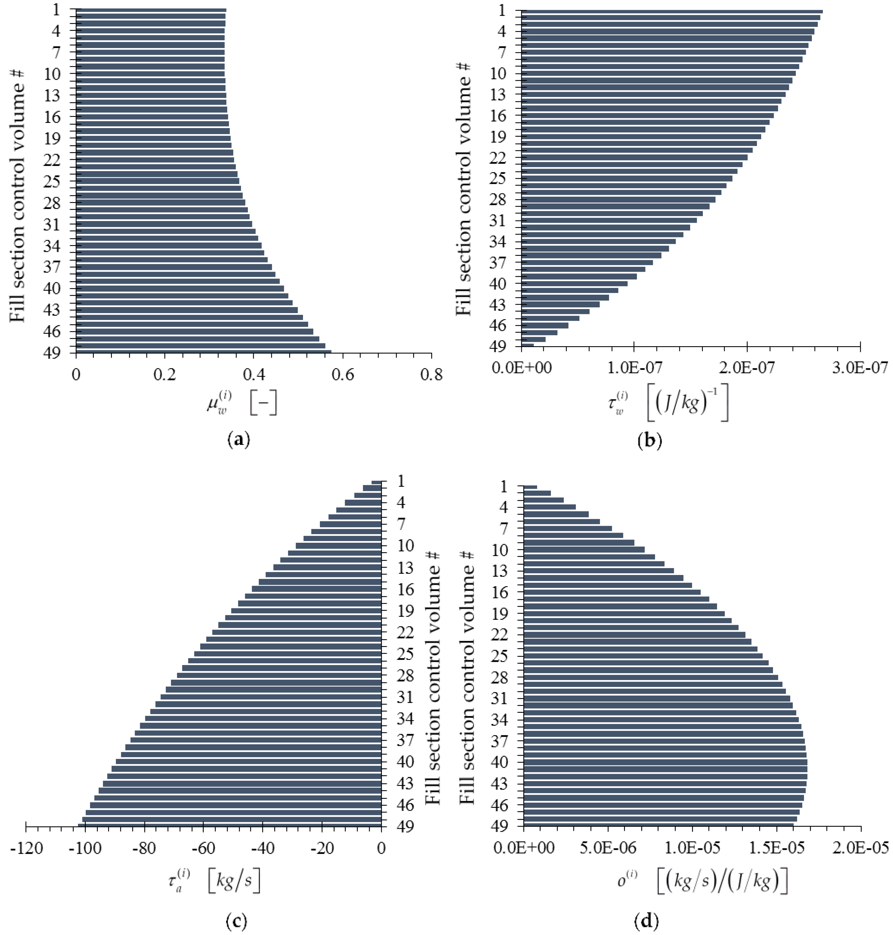
© 2016 by the authors; licensee MDPI, Basel, Switzerland. This article is an open access article distributed under the terms and conditions of the Creative Commons Attribution (CC-BY) license (http://creativecommons.org/licenses/by/4.0/).