1. Introduction
Aluminum alloys have drawn more and more attention in aerospace engineering, automotive, and electronics industries due to their low density, high specific strength, good corrosion resistance, and good recycling ability [
1,
2]. Aluminum profile is an application form of aluminum alloys, and the demand for it is extremely large because of the massive use of space-frame constructions in high-speed rail and auto body [
3]. Therefore, the surface quality of aluminum profiles has assumed significant importance. Any surface defects, such as cracks and deformations, will greatly affect the performance, safety, and reliability of products. Traditionally, human-based visual inspection is a common detection method in manufacturing engineering. However, due to low sampling rate, low precision, poor real-time performance, fatigue, greatly influenced by artificial experience, and other adverse factors, the artificial inspection is not sufficient to guarantee the stability and accuracy of detection. In addition, the other methods based on various signals, like electrical signal and magnetic signal, were also utilized to detect the surface defects by many companies. Asea Brown Boveri (ABB) Metallurgy [
4] developed the Decraktor detection unit P1 using the principle of multi-frequency eddy current testing. The device can suppress the influence of various interference noises, thereby improving the reliability of the steel plate detection. However, eddy current testing can only detect conductors and needs to be close to the surface being inspected. Besides, the rough surface affects the detection result and the penetration depth of eddy current detector is limited.
Machine vision-based method for surface defect detection has an absolute advantage in terms of its safety, reliability, convenience, and efficiency. It is an effective means to realize the automation and intellectualization of the manufacturing processes in the steel and iron industry [
5,
6]. A typical machine vision-based defect-detection method consists of light source, Charge Coupled Device (CCD) camera, and image processing algorithms [
7]. Many scholars have conducted significant research on image processing algorithms. In [
8], Chondronasios A et al. used gradient-only co-occurrence matrices (GOCM) to classify two types of defects in an extruded aluminum profile. Besides, there is not much literature about aluminum profile defect detection using machine vision technology. Nevertheless, the problem can be seen as defect detection in metal material, such as steel and iron, which has been studied for many years in computer vision.
Mathematical morphology is a technique of image analysis based on set theory, topology, and random functions. Dupont et al. [
9] proposed a method using the cost matrix theory based on mathematical morphology, and the K-nearest neighbor (KNN) [
10] classifier to detect eight kinds of defects on flat steel products. Spatial filtering is an image processing method that directly manipulates the pixels in an image. The gradient filters, like Sobel, Robert, Canny, and Laplacian filters are popular tools to detect points, lines, and edges in spatial filtering. Guo et al. [
11] used the Sobel gradient operator and Fisher discriminant to detect defects on the steel surface. Moreover, Wu et al. [
12] adopted a method based on fast Fourier transform (FFT) combined with a local border search algorithm for the recognition of hot-rolled steel strips. In [
13], Yazdchi et al. applied a multifractal-based segmentation method to detach the region of defects from images, and then extracted ten features from the detected region for classification. A method in [
14] using the Markov random field for texture analysis combined with a KNN classifier was used for classification of steel surface defects.
Although traditional machine vision-based methods using the CCD camera and image processing algorithms achieved the automatic detection of surface defects, the hand-designed features [
15] used in the defect detection needed to be carefully designed by a programmer who well understands the domain of the task, which lacks robustness and is not conducive to the identification, classification, and detection of surface defects.
In recent years, due to the advances of artificial intelligence and deep learning, more concretely the convolutional neural network (CNN) [
15,
16], the quality of image classification, object detection, and face recognition have been rapidly developed. Deep learning which is based on artificial neural network discovers the distributed representation of its input data by transforming the data and low-level features into a more abstract and composite representation; the CNN can learn highly abstract and invariable features from large training datasets automatically, rather than constructing low-level features artificially; therefore, it can be robustly adapted to various computer vision tasks.
In 2012, as the winner of the ImageNet Large Scale Visual Recognition Challenge (ILSVRC) [
17,
18], Krizhevsky et al. [
15] rekindled interests in CNN by firstly using deeper and wider networks in computer vison tasks. In [
19], Girshick et al. proposed region-based CNN (R-CNN) which uses selective search [
20] to generate around 2000 region proposals and “AlexNet” [
15] to extract features, and a set of Support Vector Machines (SVMs) [
21] and a regression model to classify and localize objects. However, the Region-CNN (R-CNN) is computationally expensive and slow, and not widely used in actual applications because it requires thousands of forward computations from the CNN to perform object detection for a single image. To address the drawbacks of R-CNN, Fast R-CNN [
22] was developed by Girshick et al. Fast R-CNN only performs CNN forward computation on the image as a whole, so it shows higher speed and accuracy than R-CNN. Despite the better performance, Fast R-CNN generates many proposed regions through an external method like selective search which is time consuming. In 2016, a region proposal network (RPN) was presented to generate nearly cost-free region proposals in [
23], and Ren et al. introduced the Faster R-CNN by combining the RPN and Fast R-CNN for object detection. The Faster R-CNN reduces the computational cost through sharing convolutional features between RPN and Fast R-CNN. Moreover, the novel RPN also improves the overall precision of object detection.
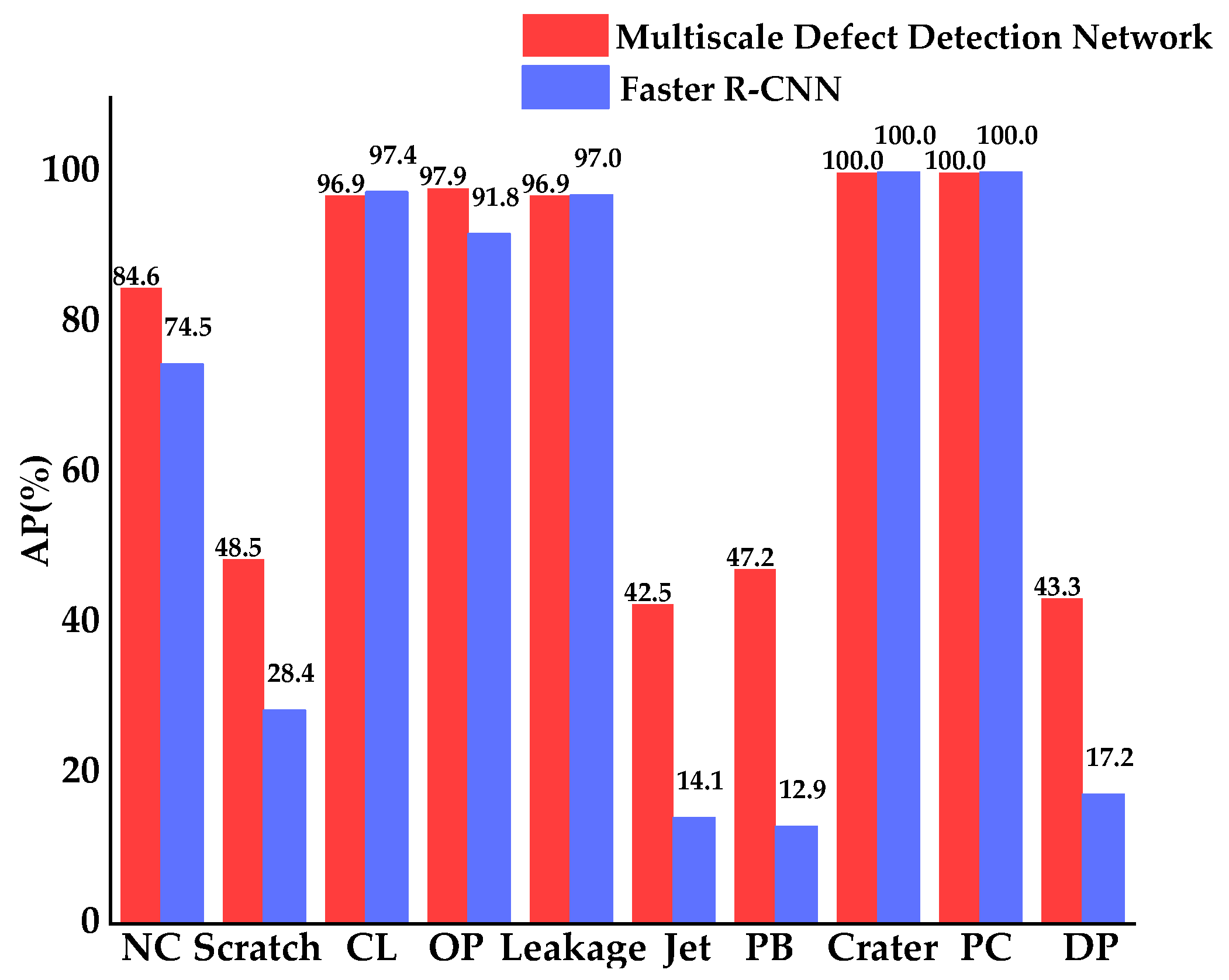
In computer vision, the objects of deep learning are often natural images, including pedestrians, vehicles, animals, and human faces, etc., but there are few studies on aluminum profile surface defects detection using the deep learning. Therefore, in this paper, we propose a multiscale defect-detection network for detecting the aluminum profile surface defects, which was based on the use of CNNs. The network is based on Faster R-CNN and the feature pyramid network (FPN) [
24], and can effectively detect surface defects with various scales.
The rest of this paper is organized as follows. In
Section 2, the dataset for training and evaluating the network is described. The multiscale defect-detection network is presented in
Section 3, including the architecture of the network and how to train the network.
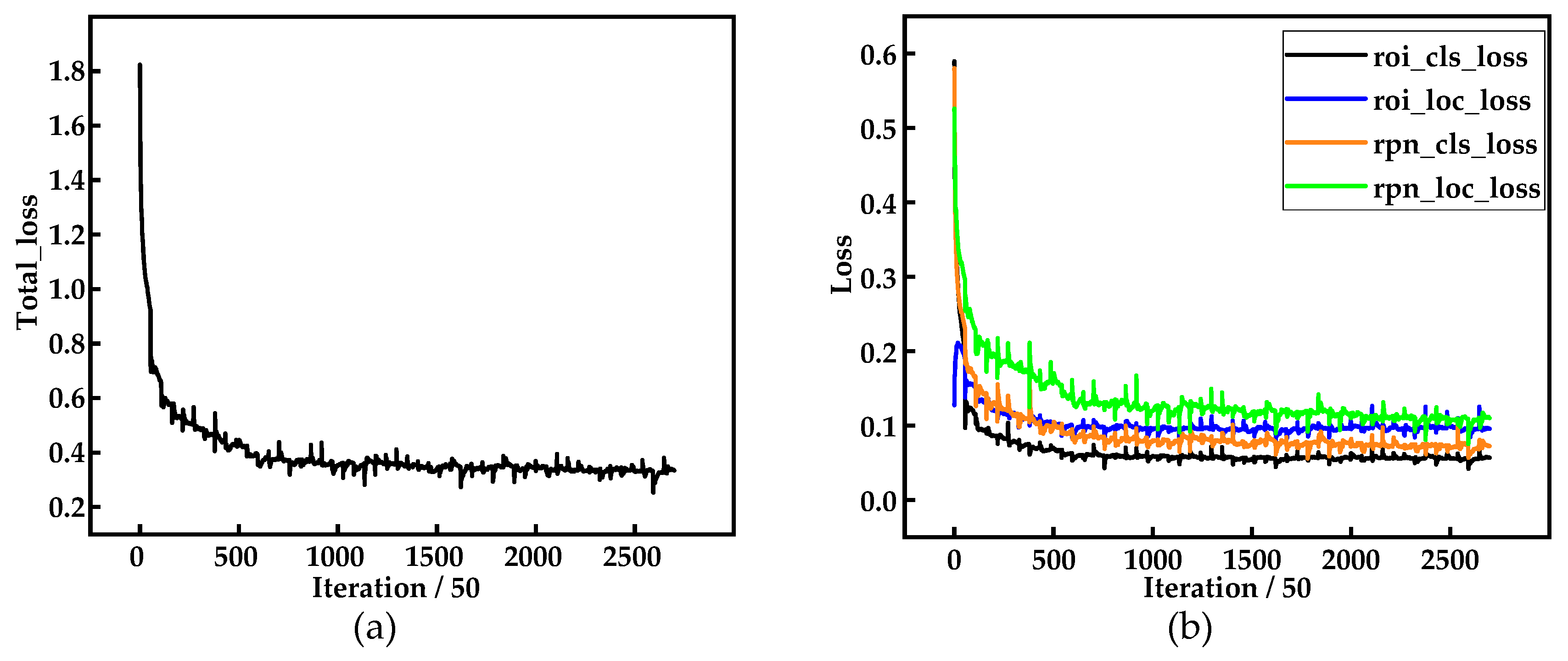
Section 4 gives an experiment for training the network, including the implementation details of the experiment and the loss in the training process. In
Section 5, the evaluation results of the network are presented. The paper ends with a summary of the major findings in
Section 6.
3. Method
To classify and localize defects on the aluminum profile surface, the multiscale defect-detection network based on Faster R-CNN was proposed. The overall schematic architecture of the network is presented in
Figure 4. The Faster R-CNN system was composed of Feature Extraction Network (FEN), Region Proposal Network (RPN), Region-of-Interesting (ROI) Pooling, and Classification and Regression Layer. Considering the characteristics of surface defects of aluminum profiles, the idea of feature fusion from FPN was added to the basic Faster R-CNN to improve defect detection performances. The details of the multiscale defect detection are explained in this section.
3.1. Feature Extraction Network
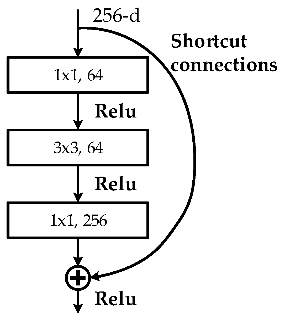
FEN is a large CNN that can automatically extract high-level features from input images. In this study, we used ResNet101 [
27] to obtain high-level and semantically strong features. The basic structure of the ResNet101 is a
bottleneck which solves the network performance degradation problem and leads the CNN model deeper than ever. As depicted in
Figure 5, the
bottleneck contains three convolutional layers: 1 × 1, 3 × 3, and 1 × 1 convolutional layers, which is followed by a “Relu” activation function [
28], respectively, and “shortcut connections,” which are those skipping one or more layers and map input directly to output without adding extra parameters.
The detailed architecture of the ResNet101 for ImageNet is summarized in
Table 1. The network was composed of
conv1,
pool,
conv2_x,
conv3_x,
conv4_x,
conv5_x, average pool, 1000 d full-connected layer (1000 d fc). The output of the fully connected layer was fed to a 1000-way softmax which could produce a probability distribution over 1000 classes. When applied to extract feature maps, we only use the
conv1,
pool,
conv2_x,
conv3_x,
conv4_x, and
conv5_x. The
conv2_x,
conv3_x,
conv4_x, and
conv5_x were constructed by
bottlenecks stacked upon each other, and the number of
bottlenecks of each section is shown in
Table 1. Because of the “very deep” network, high-level semantic features that facilitate subsequent recognition could be obtained from the
conv5_x.
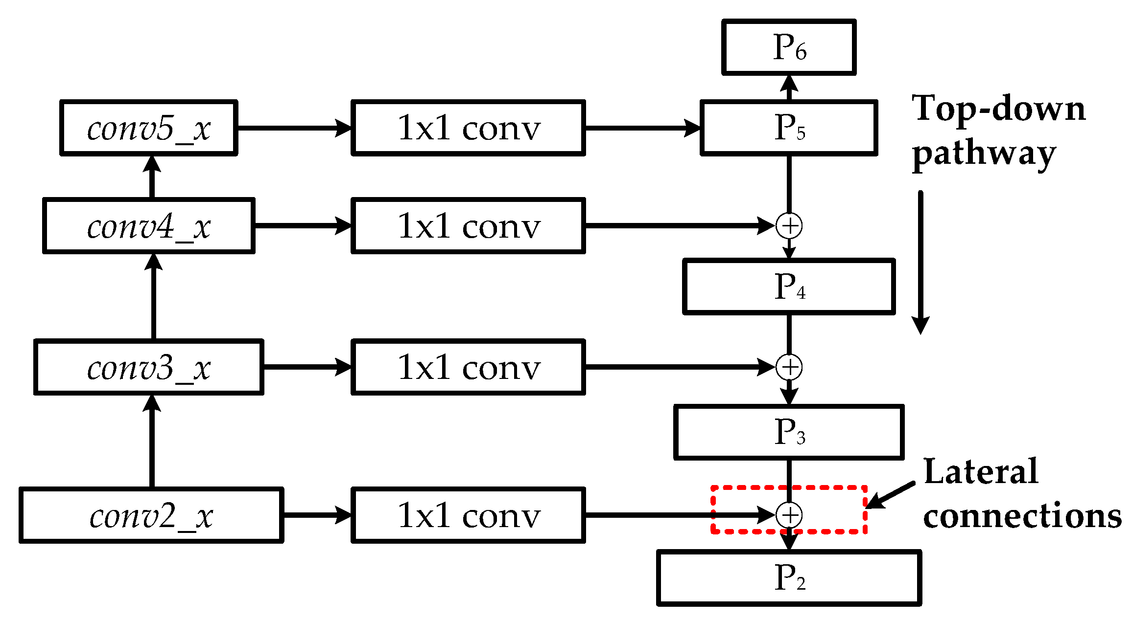
However, the high-level feature maps are usually low-resolution; so when small scale defects on the aluminum profile were mapped into high-level features, the representational capacity for the detection of these defects was weakened. The idea of feature fusion is to combine low-resolution, semantically-strong features with high-resolution, low-level features. As shown in
Figure 6, the architecture of feature fusion in the multiscale defect-detection network adopted a top-down pathway and lateral connections. The top-down pathway produced higher resolution and semantically stronger features by up-sampling semantically stronger, but lower resolution feature maps to nearest lower level features’ scale, and then these features were added to the nearby low-level features via lateral connections. Therefore, a set of multiscale feature maps: {P
2, P
3, P
4, P
5} in which all levels are semantically strong were generated. In addition, an extra feature map P
6, which is a simple two-stride subsampling of P
5, was added to the output feature maps. It is worth noting that the feature maps {P
2, P
3, P
4, P
5, P
6} would be transmitted to RPN and only {P
2, P
3, P
4, P
5} would be input into ROI pooling.
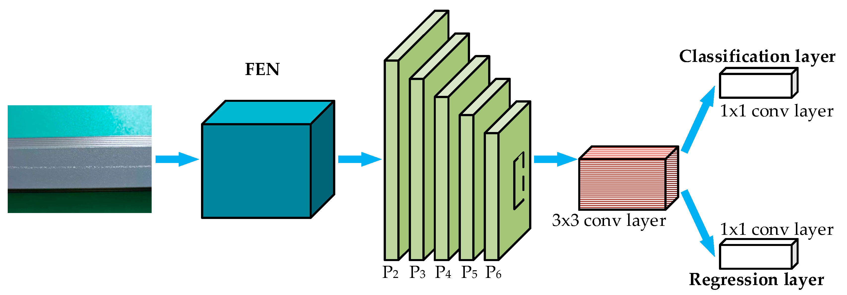
3.2. Region Proposal Network
After feature fusing, RPN can generate region proposals or regions of interest (ROI), which are rectangular regions surrounding defects, including the probability of being foreground (containing defects) in each proposal. The schematic structure of an improved RPN is presented in
Figure 7. The improved RPN is a fully convolutional network, which is naturally implemented with a 3 × 3 convolutional (conv) layer followed by two sibling 1 × 1 convolutional (conv) layers for classification and regression. Concretely, we attach the fully convolutional network (3 × 3 conv and two 1 × 1 convs) to each feature map output by FEN, and then several vectors containing estimate probability of defect/not-defect for each anchor and prediction coordinate transformation from anchors to region proposals are generated.
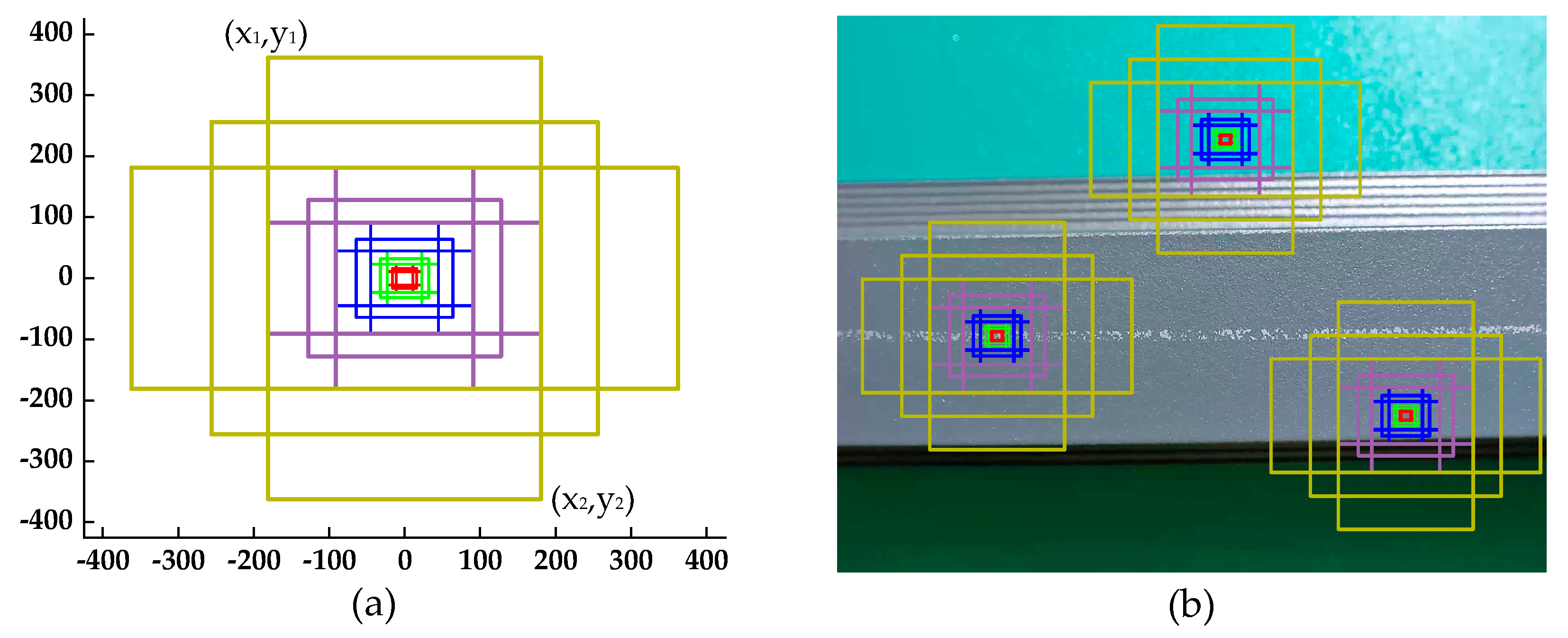
Anchors play an important role in the improved RPN. An anchor is a reference box, determined by upper left and lower right coordinates: (x
1, y
1) and (x
2, y
2), as shown in
Figure 8a. The anchor which is previously assigned on the input image transforms the defect detection problem into whether the anchor surrounds any defects and how far away the defect is from the anchor (shown in
Figure 8b). Based on the work of Lin et al. [
24], we defined the anchors to have areas of {32
2, 64
2, 128
2, 256
2, 512
2} pixels corresponding to {P
2, P
3, P
4, P
5, P
6} in the improved RPN. Moreover, the anchor in each feature map has three aspect ratios: {1:2, 1:1, 2:1}. In the improved RPN, there are 15 kinds of anchors, and approximately 306,900 anchors set on the input image.
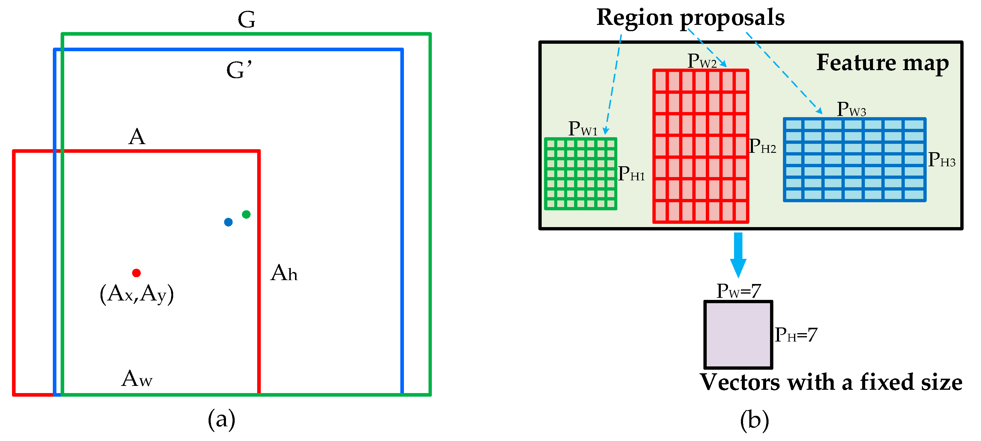
Although the improved RPN could create a large number of anchors, some of which may be close to defects, these anchors provide coarse localization and need to be refined. The regression layer is a simple, inexpensive technique which can compensate for the anchors’ weakness at localization. Concretely, it attempts to learn a transformation d × (A) that maps the anchors to the region proposal. As described in
Figure 9a, A is the anchor, G is the ground truth box, and G’ is the predicting region proposal, which are specified as a set of center coordinates and a width and height in pixels, where A = (A
x, A
y, A
w, A
h). Thus, the transformation d × (A) could transform A into G’ which is closer to G and better captures the defect:
3.3. ROI Pooling
The region proposals output from the improved RPN have different dimensions, and the input of final classification and regression layer need to be the same size, so the purpose of ROI pooling is to perform max pooling to convert the features inside any proposals into vectors with a fixed size (e.g., 7 × 7). The specific operation of ROI pooling is shown in
Figure 9b. Firstly, the region proposals with different sizes are divided into equal-sized sections, such as 7 × 7; then, the max value in each section is output, and fixed-size vectors can be obtained.
In addition, the region proposal with (x
1, y
1) and (x
2, y
2) need to be mapped to the feature maps before the operation ROI pooling. There are four feature maps {P
2, P
3, P
4, P
5} input into ROI pooling, so it is important to determine which feature map the region proposal belongs to. As per Lin [
24], we assigned a region proposal of width (w) and height (h) (on the input image) to the feature map P
k by:
Intuitively, if the region proposal’s scale is 512 × 512, it should be mapped to P5. The mapping method is to reduce coordinates of the anchor to the down-sampling multiple of the input image to the feature map. For example, we defined the anchor with area of 5122 pixels on the P5 feature map. Therefore, one anchor which is center at the input image with scale {−256, 256, 256, −256 } is {−8, 8, 8, −8} when mapped to P5.
3.4. Classification and Regression Layers
The classification and regression layers are composed of fully-connected layers. For the classification layer, it outputs a vector with the predicting probability of 11 classes (10 defects plus 1 background class); the regression layer outputs four parameters for each class to refine the region proposals again. Before the final classification and regression layer, there are two hidden, 1024 d fully connected layers which map the learned features to the sample space for classification and regression.
3.5. Network Training
The multiscale defect-detection network is composed of the architecture of the network and weights of the convolutional layers. When the design of the network structure was completed, we needed to obtain the optimal weights of the convolutional layers. Network training is a process that realizes the optimization of weights and leads the prediction of the network approximating to the truth of inputs, and it consists of forward propagation and backward propagation. Forward propagation is the calculation and storage of intermediate variables (including outputs) for the network in the order from input to output. Backward propagation refers to the method of calculating the losses (the difference between outputs and the truth of inputs) of the network and updating the weights using the gradient from the losses. The losses of the multiscale defect-detection network are from the improved RPN and the Classification and Regression layers. In the training, the selection of the losses is extremely significant.
The improved RPN is trained end-to-end, for both the classification and regression layers. We used the multitask loss L in Fast R-CNN [
22] to train the improved RPN:
where i is the index of an anchor in a mini-batch, and in the classification loss p* and p are the ground truth label and predicted probability of being defects in the anchor, respectively. In the regression loss, t
i and t
i* are vectors representing the geometrical difference between the anchor and the predicting region proposal, as well as the anchor and the ground truth box, respectively, and t
i* is calculated as:
Additionally, the classification loss is calculated as:
The regression loss is calculated as:
Moreover, we use the same loss as the improved RPN to train the Classification and Regression layers, which are also trained end-to-end.


