Artificial Neural Networks in Classification of Steel Grades Based on Non-Destructive Tests

 ,
,  ,
,  ,
, 
Abstract
:
1. Introduction
- (a) Random nature, which is their objective property and because of imperfections in the structure of the material. This circumstance requires the involvement of the apparatus of probability theory and mathematical statistics for the organization of control and certification of products;
- (b) The interdependence of mechanical properties, which requires the simultaneous determination of a set of strength characteristics on any part of the structure;
- (c) The dependence of mechanical properties on the loading history, which takes place in operation and transforms a random variable into a random function.
2. Materials and Methods
- The dimensions of the device are significantly reduced, which makes it available in any part of the structure;
- For most designs, dynamic loading is more dangerous than static;
- The reaction of the material to the dynamic effect is more informative, which allows not only to evaluate the mechanical properties but also to develop effective technological operations (shot blasting, surface-plastic deformation, explosion, etc.);
- φ change in the strain rate during testing can noticeably change the mechanical properties of the material, which is associated with a transition to another mechanical state (for example, in metals, from plastic-viscous to brittle; in polymers, from highly elastic to elastic). The appearance of a viscous-brittle fracture is extremely dangerous for metals since it leads to cracking and fracture. A viscous-brittle breach can only be predicted based on appropriate tests.
- Low speeds (up to 10 m/s). It is generally accepted (Fridman [33]) that, in this case, wave processes and inertial forces do not significantly affect the reaction of the material and can be neglected. Most quasi-static impact models are applicable for this speed range. At the same time, it is incorrect to assume that the low strain rate does not affect the mechanical properties of the material. As experiments [34,35] show, the dynamic properties of the material (yield and strength limits, elongation and narrowing) significantly (up to two times) differ from static ones, which is associated with the processes of nucleation, development, and movement of dislocations, as well as with the diffusion rate chemical and physical processes, both inside the loaded body, and at the border with the environment.
- High speeds (from 10 to 100 m/s). In this case, the inertial resistance of the material is substantial; the unevenness of the stress and strain states is great. The resistance of a material to pushing a solid striker into it increases in proportion to the square of the speed according to the lawwhere:—the resistance at low speed; —static component; —the speed of the striker; and n—empirical coefficients depending on the speed of the striker; —the density of the half-space material.
- Ultrahigh and hyper high speeds (from 100 m/s and above). At ultra-high speeds, the resistance increases even more, sometimes reaching an elastic modulus. It is generally accepted that at such rates, the hydrodynamic theory of flow is applicable to the material.
3. Results
- The automatic search for ten of the best classifying networks (out of 1000 found);
- The manual choice, at least eight ANNs (out of ten proposed) providing a high level of correct classification in every subset (training, testing and validating);
- Making predictions for all 67 cases based on the ensemble of the chosen networks (retaining information which case belongs to each subset).
4. Discussion
- If the result from Step 1 classified the sample to grey class, the class of steel is 1 96 HB with 100% confidence (it stops the reasoning), if not, take Step 2;
- If the result from Step 2 classified the sample to grey class, the class of steel is 2 96 HB with 100% confidence (it stops the reasoning), if not, take Step 3;
- If the result from Step 3 classified the sample to grey class, the class of steel is 3 182 HB with 100% confidence (it stops the reasoning). Five out of 42 classifications in Step 3 are incorrect i.e., falsely classified to 4 195 HB (but at this moment, it is assumed that Step 3 classified to the grey class; it stops the procedure). If Step 3 classified the sample to the violet class, take Step 4;
- If the result from Step 4 classified the sample to grey class, the class of steel is 4 195 HB with confidence (it stops the procedure). In six cases out of 48 it can belong to 5 197 HB. If the sample is classified to the violet class, go to Step 5;
- If Step 5 classified the sample to the grey class, the sample is 5 197 HB in 100% confidence (there is one case falsely classified to the violet class, but for this moment it is assumed that Step 5 classified the sample to the grey class); if Step 5 classified the sample to the violet class, go to Step 6;
- If Step 6 classified the sample to the grey class, the sample is 6 271 HB in 100% confidence, if not, go to Step 7;
- If Step 7 classified the sample to the grey class, the sample is 7 442 HB with confidence (it stops the procedure). This one case from class 9 450 HB can be classified as belonging to the grey class. If the sample is classified to the violet class, go to Step 8;
- If Step 8 classified the sample to the grey class, the sample is 8 446 HB with confidence, if not (the class pointed by Step 8 is violet) the sample belongs to 9 450 HB with confidence equals to (this ends the procedure).
5. Conclusions
Author Contributions
Funding
Acknowledgments
Conflicts of Interest
Appendix A

| Time in ms | 1 96 HB | 2 96 HB | ||||||||||||
|---|---|---|---|---|---|---|---|---|---|---|---|---|---|---|
| Test 1 | Test 2 | Test 3 | Test 4 | Test 5 | Test 6 | Test 7 | Test 8 | Test 9 | Test 10 | Test 11 | Test 12 | Test 13 | Test 14 | |
| 0.01 | −0.3508 | −1.2392 | −0.7800 | −0.3720 | −0.7948 | 0.3948 | −1.3889 | −0.7233 | −0.2569 | −0.8946 | −0.1574 | −0.6031 | −0.1621 | −0.7674 |
| 0.02 | 0.8505 | 0.2169 | 0.9772 | 1.3952 | 0.5525 | 1.8073 | −0.3889 | 0.7866 | 1.0193 | 0.6470 | 0.9928 | 0.8598 | 1.1990 | 0.6386 |
| 0.03 | 2.3081 | 1.8648 | 2.7355 | 3.2623 | 2.1400 | 3.4737 | 0.8846 | 2.3011 | 2.4683 | 2.1594 | 2.3879 | 2.3138 | 2.7697 | 2.0471 |
| 0.04 | 4.0649 | 3.7459 | 4.5665 | 5.2294 | 3.9830 | 5.3565 | 2.4212 | 3.8948 | 4.1433 | 3.7607 | 4.0571 | 3.8592 | 4.5581 | 3.5759 |
| 0.05 | 5.8770 | 5.7252 | 6.4610 | 7.0958 | 5.7402 | 6.8921 | 4.0692 | 5.6010 | 5.6715 | 5.5750 | 5.5447 | 5.5855 | 6.1406 | 5.2862 |
| 0.06 | 7.8200 | 7.6150 | 8.2141 | 8.8518 | 7.4882 | 8.4192 | 5.7667 | 7.2728 | 7.2566 | 7.1956 | 7.0766 | 7.2469 | 7.7005 | 6.8505 |
| 0.07 | 9.7782 | 9.4424 | 9.8919 | 10.5500 | 9.2761 | 10.0778 | 7.4713 | 8.8498 | 8.9049 | 8.7501 | 8.7189 | 8.8507 | 9.3372 | 8.4491 |
| 0.08 | 11.2408 | 10.9870 | 11.4036 | 11.9153 | 10.6403 | 11.2272 | 9.0468 | 10.2758 | 10.1794 | 10.2998 | 9.9402 | 10.3225 | 10.6131 | 9.9714 |
| 0.09 | 12.4967 | 12.2547 | 12.5650 | 13.0021 | 11.8679 | 12.3611 | 10.4838 | 11.4529 | 11.3794 | 11.4537 | 11.1498 | 11.4954 | 11.8388 | 11.2015 |
| 0.10 | 13.5303 | 13.3822 | 13.5697 | 13.9052 | 12.9176 | 13.2439 | 11.7424 | 12.4812 | 12.3719 | 12.5519 | 12.1794 | 12.5813 | 12.8921 | 12.4534 |
| 0.11 | 14.0830 | 14.0312 | 14.1076 | 14.3014 | 13.4789 | 13.6249 | 12.6816 | 13.1811 | 12.9867 | 13.3765 | 12.7508 | 13.3403 | 13.4690 | 13.3283 |
| 0.12 | 14.4026 | 14.3853 | 14.1923 | 14.3610 | 13.8520 | 13.9797 | 13.3673 | 13.6478 | 13.4576 | 13.7732 | 13.2762 | 13.8063 | 13.9224 | 13.9195 |
| 0.13 | 14.3485 | 14.4396 | 14.1381 | 14.2186 | 13.8872 | 13.8809 | 13.8853 | 13.9450 | 13.6332 | 14.1298 | 13.5053 | 14.1770 | 14.1208 | 14.3962 |
| 0.14 | 13.8763 | 13.8507 | 13.5035 | 13.4419 | 13.4531 | 13.2876 | 13.9832 | 13.6443 | 13.3486 | 13.9755 | 13.2832 | 13.9750 | 13.7603 | 14.2588 |
| 0.15 | 13.1391 | 12.9529 | 12.5113 | 12.3016 | 12.7237 | 12.3974 | 13.7171 | 13.0927 | 12.7166 | 13.3392 | 12.8608 | 13.4170 | 13.0586 | 13.8311 |
| 0.16 | 11.9428 | 11.7584 | 11.2767 | 10.8988 | 11.5043 | 11.0035 | 13.0962 | 12.1645 | 11.6494 | 12.4444 | 11.9743 | 12.5036 | 11.9368 | 13.0117 |
| 0.17 | 10.3662 | 10.1259 | 9.5892 | 9.0303 | 9.9132 | 9.4642 | 11.9338 | 10.7371 | 10.2645 | 10.9936 | 10.6956 | 11.0684 | 10.4768 | 11.5979 |
| 0.18 | 8.6348 | 8.4701 | 7.8503 | 7.2157 | 8.2931 | 7.8269 | 10.5571 | 9.3761 | 8.8065 | 9.3850 | 9.3225 | 9.6272 | 8.9571 | 10.1864 |
| 0.19 | 6.6833 | 6.5507 | 5.9265 | 5.2652 | 6.4434 | 5.8484 | 8.9920 | 7.6853 | 7.1061 | 7.6878 | 7.6431 | 7.9364 | 7.1844 | 8.4579 |
| 0.22 | 4.6213 | 4.3220 | 3.7560 | 3.0096 | 4.4085 | 3.8055 | 7.1724 | 5.6273 | 5.2234 | 5.6248 | 5.7770 | 5.8720 | 5.1271 | 6.3478 |
| 0.21 | 2.5593 | 2.1925 | 1.6386 | 1.0427 | 2.3965 | 1.6632 | 5.2772 | 3.6783 | 3.2178 | 3.5421 | 3.8399 | 3.7848 | 3.0005 | 4.3294 |
| 0.22 | 0.4300 | −0.0323 | −0.5883 | −0.9692 | 0.2011 | −0.5579 | 3.2044 | 1.4385 | 0.9883 | 1.4271 | 1.6349 | 1.4458 | 0.7932 | 2.0115 |
| 0.23 | −1.5755 | −2.2013 | −2.6915 | −3.1130 | −1.9471 | −2.4908 | 1.0298 | −0.7383 | −1.1490 | −0.7774 | −0.5461 | −0.8400 | −1.2988 | −0.3248 |
| 0.24 | −3.3927 | −4.0719 | −4.4561 | −4.9430 | −3.7743 | −4.2951 | −1.0532 | −2.5237 | −3.0815 | −2.6818 | −2.5856 | −2.7677 | −3.1282 | −2.2338 |
| 0.25 | −5.1410 | −5.8582 | −6.1562 | −6.7084 | −5.4778 | −5.9781 | −2.9906 | −4.3841 | −4.8812 | −4.4363 | −4.5134 | −4.6636 | −4.8291 | −4.1654 |
| 0.26 | −6.7028 | −7.4217 | −7.5659 | −8.2543 | −6.9447 | −7.3340 | −4.6446 | −5.9917 | −6.3977 | −6.0862 | −6.0945 | −6.3345 | −6.3415 | −5.9272 |
| 0.27 | −8.1060 | −8.7440 | −8.8247 | −9.3883 | −8.1872 | −8.6371 | −6.1539 | −7.3377 | −7.7813 | −7.4611 | −7.5246 | −7.7622 | −7.7313 | −7.3619 |
| 0.28 | −9.4308 | −10.0618 | −10.0734 | −10.4814 | −9.4013 | −9.8474 | −7.6005 | −8.7289 | −9.0939 | −8.7920 | −8.8773 | −9.1603 | −9.0241 | −8.8288 |
| 0.29 | −10.5393 | −11.1304 | −11.0829 | −11.4828 | −10.4654 | −10.8252 | −8.8542 | −9.8390 | −10.2159 | −10.0130 | −9.9946 | −10.3412 | −10.1753 | −10.0420 |
| 0.30 | −11.5197 | −12.0557 | −12.0217 | −12.3401 | −11.4168 | −11.7797 | −10.0379 | −10.8211 | −11.2662 | −11.0119 | −11.0858 | −11.3907 | −11.2828 | −10.9799 |
| 0.31 | −12.4276 | −12.9317 | −12.8454 | −13.1442 | −12.2413 | −12.5273 | −11.1095 | −11.8173 | −12.1609 | −11.9450 | −12.0340 | −12.4034 | −12.2643 | −11.9874 |
| 0.32 | −13.1572 | −13.5257 | −13.3978 | −13.7140 | −12.8621 | −13.0696 | −11.9939 | −12.5192 | −12.8999 | −12.7198 | −12.7691 | −13.1876 | −13.0484 | −12.8375 |
| 0.33 | −13.8296 | −14.0679 | −13.8539 | −14.1916 | −13.4695 | −13.6546 | −12.8243 | −13.2000 | −13.5708 | −13.3268 | −13.4831 | −13.8349 | −13.7340 | −13.5538 |
| 0.34 | −14.3406 | −14.4953 | −14.1230 | −14.6030 | −13.8975 | −14.0229 | −13.5214 | −13.7844 | −14.0340 | −13.8729 | −13.9197 | −14.3207 | −14.1727 | −14.1770 |
| 0.35 | −14.5470 | −14.5914 | −14.1781 | −14.7470 | −14.0830 | −14.2091 | −14.0271 | −14.1316 | −14.3557 | −14.2004 | −14.1699 | −14.5892 | −14.3925 | −14.4972 |
| 0.36 | −14.5844 | −14.6381 | −14.2405 | −14.6969 | −14.2147 | −14.3101 | −14.4621 | −14.4428 | −14.5312 | −14.3326 | −14.4048 | −14.7493 | −14.5105 | −14.6901 |
| 0.37 | −14.4179 | −14.5078 | −14.0968 | −14.4076 | −14.0738 | −14.1258 | −14.6925 | −14.4777 | −14.4379 | −14.3133 | −14.3944 | −14.6952 | −14.4241 | −14.7291 |
| 0.38 | −14.1370 | −14.1243 | −13.8027 | −13.9065 | −13.8475 | −13.8117 | −14.6622 | −14.2696 | −14.2433 | −14.0602 | −14.2411 | −14.4195 | −14.1716 | −14.4826 |
| 0.39 | −13.8485 | −13.7296 | −13.4501 | −13.4287 | −13.7780 | −13.3996 | −14.4699 | −14.0689 | −13.9123 | −13.7201 | −13.9522 | −14.0385 | −13.7795 | −14.1539 |
| 0.40 | −13.4108 | −13.2112 | −12.9393 | −12.9001 | −13.4401 | −12.7873 | −14.0537 | −13.6463 | −13.3969 | −13.2759 | −13.4237 | −13.4918 | −13.2149 | −13.6420 |
| 0.41 | −12.8457 | −12.5340 | −12.3927 | −12.1717 | −12.8061 | −12.1068 | −13.5315 | −13.1215 | −12.7578 | −12.6833 | −12.8352 | −12.7506 | −12.4988 | −12.8958 |
| 0.42 | −12.1135 | −11.6385 | −11.6675 | −11.0288 | −11.9395 | −11.1055 | −12.9520 | −12.4983 | −11.8153 | −11.9529 | −12.0885 | −11.7198 | −11.4634 | −11.9564 |
| 0.43 | −11.0301 | −10.2406 | −10.5175 | −9.2847 | −10.5545 | −9.5836 | −12.0917 | −11.3041 | −10.3739 | −10.8004 | −10.8922 | −10.1670 | −9.8849 | −10.4850 |
| 0.44 | −9.5532 | −8.3835 | −8.9507 | −7.1051 | −8.7744 | −7.6217 | −10.8090 | −9.6128 | −8.4383 | −9.1383 | −9.2107 | −8.1262 | −7.8192 | −8.4506 |
| 0.45 | −7.6392 | −6.1882 | −6.9483 | −4.6887 | −6.7327 | −5.1849 | −9.0098 | −7.4556 | −6.0595 | −7.1354 | −7.0192 | −5.7195 | −5.3124 | −6.0490 |
| 0.46 | −5.4027 | −3.8942 | −4.7510 | −2.2925 | −4.3576 | −2.7023 | −6.7391 | −4.9239 | −3.4959 | −4.8757 | −4.5910 | −3.1895 | −2.6107 | −3.4388 |
| 0.47 | −3.2150 | −1.9201 | −2.7452 | −0.2548 | −1.9743 | −0.7200 | −4.3031 | −2.4895 | −1.1295 | −2.6682 | −2.2772 | −0.9511 | −0.2487 | −1.0755 |
| 0.48 | −1.3537 | −0.4604 | −1.0882 | 1.2331 | −0.0636 | 0.6779 | −1.9638 | −0.4664 | 0.6644 | −0.8344 | −0.3370 | 0.7829 | 1.4233 | 0.6640 |
| 0.49 | −0.0197 | 0.3326 | −0.0765 | 1.9724 | 1.2048 | 1.3128 | −0.1305 | 0.9604 | 1.6997 | 0.5222 | 0.9591 | 1.8669 | 2.3408 | 1.6887 |
| 0.50 | 0.6677 | 0.5075 | 0.2580 | 2.0366 | 1.8408 | 1.3407 | 0.9929 | 1.6566 | 2.0878 | 1.2477 | 1.6501 | 2.2716 | 2.5009 | 1.9937 |
| 0.51 | 0.8367 | 0.3152 | 0.1343 | 1.7155 | 1.8535 | 1.1203 | 1.5336 | 1.8055 | 1.9503 | 1.4441 | 1.8406 | 2.1861 | 2.1010 | 1.7834 |
| 0.52 | 0.5985 | −0.1124 | −0.2818 | 1.1456 | 1.4203 | 0.7647 | 1.5087 | 1.5650 | 1.4699 | 1.3166 | 1.6210 | 1.7222 | 1.5094 | 1.2562 |
| 0.53 | 0.1303 | −0.6313 | −0.7335 | 0.5439 | 0.8309 | 0.3870 | 1.1750 | 1.1395 | 0.9172 | 0.9978 | 1.1871 | 1.0692 | 0.8477 | 0.5620 |
| 0.54 | −0.3245 | −1.0681 | −1.1115 | −0.0063 | 0.1972 | −0.0103 | 0.8045 | 0.7045 | 0.3472 | 0.6773 | 0.6634 | 0.4405 | 0.1106 | −0.1577 |
| 0.55 | −0.6910 | −1.4494 | −1.4329 | −0.5581 | −0.3517 | −0.4505 | 0.3825 | 0.1827 | −0.2499 | 0.3279 | 0.1131 | −0.1455 | −0.5373 | −0.8970 |
| 0.56 | −0.9896 | −1.7407 | −1.6249 | −0.9836 | −0.7490 | −0.8670 | −0.0263 | −0.2929 | −0.7310 | −0.0752 | −0.3886 | −0.6692 | −1.1158 | −1.5602 |
| 0.57 | −1.1976 | −1.8756 | −1.6752 | −1.2610 | −1.0854 | −1.3114 | −0.4193 | −0.6743 | −1.1324 | −0.4515 | −0.8065 | −1.1864 | −1.7550 | −2.0869 |
| 0.58 | −1.3647 | −1.9545 | −1.5906 | −1.4943 | −1.4219 | −1.7427 | −0.8208 | −1.0598 | −1.5448 | −0.8914 | −1.2074 | −1.7475 | −2.3526 | −2.5807 |
| 0.59 | −1.4384 | −2.0300 | −1.4279 | −1.6775 | −1.7623 | −2.1186 | −1.2239 | −1.4209 | −1.9299 | −1.4040 | −1.6931 | −2.2437 | −2.8396 | −2.9521 |
| 0.60 | −1.4041 | −2.0266 | −1.3440 | −1.9150 | −2.0661 | −2.5143 | −1.7111 | −1.8554 | −2.2981 | −1.9499 | −2.1960 | −2.6556 | −3.1733 | −3.0968 |
| 0.61 | −1.3492 | −1.9665 | −1.2788 | −2.1657 | −2.3251 | −2.7982 | −2.1818 | −2.3611 | −2.6362 | −2.5233 | −2.6053 | −2.9164 | −3.2964 | −3.0249 |
| 0.62 | −1.2609 | −1.9140 | −1.2218 | −2.3148 | −2.5498 | −3.0312 | −2.6226 | −2.8212 | −2.9062 | −2.9745 | −2.9410 | −2.9787 | −3.2550 | −2.7111 |
| 0.63 | −1.2222 | −1.8655 | −1.2379 | −2.4515 | −2.6831 | −3.2369 | −2.9838 | −3.1759 | −3.0726 | −3.2797 | −3.0963 | −2.8884 | −3.0999 | −2.2936 |
| 0.64 | −1.3158 | −1.8113 | −1.2863 | −2.5665 | −2.7330 | −3.3120 | −3.1130 | −3.3470 | −3.1230 | −3.4071 | −3.0222 | −2.6443 | −2.8405 | −1.9470 |
| 0.65 | −1.5280 | −1.6588 | −1.4295 | −2.6633 | −2.7229 | −3.3558 | −3.0649 | −3.3440 | −3.1239 | −3.3022 | −2.8818 | −2.3568 | −2.5823 | −1.7194 |
| 0.66 | −1.8571 | −1.5695 | −1.6994 | −2.8779 | −2.6072 | −3.3159 | −2.8781 | −3.2242 | −3.0594 | −3.0833 | −2.6878 | −2.1918 | −2.4045 | −1.5895 |
| 0.67 | −2.2396 | −1.8809 | −2.0206 | −3.1185 | −2.4687 | −3.2008 | −2.6023 | −2.9585 | −2.9180 | −2.7776 | −2.5049 | −2.1406 | −2.2733 | −1.5016 |
| 0.68 | −2.5877 | −2.3709 | −2.3691 | −3.3168 | −2.3928 | −3.1196 | −2.3447 | −2.7025 | −2.7616 | −2.5334 | −2.4303 | −2.1539 | −2.1533 | −1.4824 |
| 0.69 | −2.8138 | −2.7133 | −2.6961 | −3.5357 | −2.3501 | −3.0241 | −2.1321 | −2.5188 | −2.6466 | −2.4917 | −2.4401 | −2.1917 | −2.0552 | −1.5275 |
| 0.70 | −2.9685 | −2.9626 | −2.9447 | −3.6362 | −2.3522 | −2.9676 | −2.0262 | −2.3632 | −2.5909 | −2.5046 | −2.4711 | −2.1259 | −1.9332 | −1.5846 |
| 0.71 | −3.2304 | −3.0116 | −3.1274 | −3.5612 | −2.3492 | −2.9356 | −1.9933 | −2.3150 | −2.5793 | −2.5404 | −2.5056 | −1.9918 | −1.7936 | −1.6428 |
| 0.72 | −3.4333 | −2.9509 | −3.1296 | −3.3693 | −2.3199 | −2.8330 | −1.9620 | −2.2611 | −2.5823 | −2.5512 | −2.4881 | −1.8562 | −1.7602 | −1.6454 |
| 0.73 | −3.4392 | −3.1198 | −3.0231 | −3.1085 | −2.2874 | −2.7147 | −1.9553 | −2.1328 | −2.5088 | −2.4279 | −2.4224 | −1.7003 | −1.7661 | −1.5876 |
| 0.74 | −3.3273 | −3.2600 | −3.0058 | −2.5753 | −2.1907 | −2.5562 | −1.8805 | −2.0171 | −2.3369 | −2.3162 | −2.3092 | −1.5387 | −1.4640 | −1.5654 |
| 0.75 | −3.0449 | −3.1512 | −2.9814 | −1.8205 | −2.0708 | −2.3796 | −1.7914 | −1.8852 | −2.1638 | −2.2423 | −2.1504 | −1.4223 | −1.1909 | −1.5505 |
| 0.76 | −2.7082 | −3.0758 | −2.8684 | −1.5481 | −2.0045 | −2.2545 | −1.7358 | −1.7201 | −1.9901 | −2.1220 | −2.0496 | −1.3304 | −1.4245 | −1.4687 |
| 0.77 | −2.5245 | −3.0472 | −2.6986 | −1.7668 | −1.8476 | −2.0923 | −1.6282 | −1.6145 | −1.8138 | −2.0424 | −1.9681 | −1.2928 | −1.7178 | −1.3945 |
| 0.78 | −2.3700 | −2.9247 | −2.4498 | −2.0337 | −1.6652 | −1.9292 | −1.5386 | −1.5121 | −1.6768 | −1.9553 | −1.8850 | −1.3613 | −1.8804 | −1.3908 |
| 0.79 | −2.1836 | −2.7952 | −2.2168 | −2.3743 | −1.6457 | −1.8377 | −1.5581 | −1.4660 | −1.5704 | −1.8425 | −1.8794 | −1.4436 | −2.0532 | −1.4393 |
| 0.80 | −2.0526 | −2.6406 | −2.1312 | −2.3773 | −1.6643 | −1.8020 | −1.6210 | −1.5108 | −1.5028 | −1.7435 | −1.8737 | −1.5182 | −1.8096 | −1.4778 |
| 0.81 | −1.9809 | −2.4471 | −2.1086 | −2.0006 | −1.7231 | −1.8703 | −1.6795 | −1.5905 | −1.4979 | −1.6326 | −1.8689 | −1.6918 | −1.4664 | −1.5507 |
| 0.82 | −1.9246 | −2.2852 | −2.1256 | −1.9560 | −1.8530 | −1.9456 | −1.7023 | −1.7434 | −1.5317 | −1.6559 | −1.8896 | −1.8638 | −1.5435 | −1.6715 |
| 0.83 | −1.8900 | −2.1526 | −2.1747 | −2.0227 | −1.8602 | −1.9381 | −1.7025 | −1.8891 | −1.5561 | −1.8345 | −1.8590 | −1.9526 | −1.5767 | −1.8218 |
| 0.84 | −1.9113 | −2.0537 | −2.2965 | −1.9196 | −1.7826 | −1.9620 | −1.7442 | −1.9696 | −1.5407 | −1.9365 | −1.8990 | −2.0199 | −1.5450 | −2.0060 |
| 0.85 | −1.9911 | −2.0360 | −2.4771 | −1.9145 | −1.7811 | −2.0019 | −1.8875 | −2.0642 | −1.5820 | −1.9270 | −2.0148 | −1.9990 | −1.6569 | −2.1361 |
| 0.86 | −2.1012 | −2.0623 | −2.5879 | −1.8938 | −1.9250 | −2.0153 | −2.0510 | −2.0667 | −1.7908 | −1.9167 | −2.0780 | −1.9026 | −1.7782 | −2.1361 |
| 0.87 | −2.2421 | −2.1319 | −2.7133 | −1.9511 | −2.1811 | −2.0648 | −2.1117 | −2.0298 | −2.0483 | −1.8995 | −2.1293 | −1.9301 | −1.8639 | −2.1432 |
| 0.88 | −2.3820 | −2.2239 | −2.8869 | −2.0721 | −2.3306 | −2.0814 | −2.1188 | −2.0587 | −2.2263 | −1.9662 | −2.1274 | −1.9967 | −1.9220 | −2.2337 |
| 0.89 | −2.4926 | −2.3198 | −2.9723 | −2.0656 | −2.3612 | −2.0662 | −2.1449 | −2.0355 | −2.3018 | −2.0885 | −2.0752 | −2.0227 | −1.9416 | −2.3037 |
| 0.90 | −2.5867 | −2.4120 | −3.0267 | −2.1226 | −2.3470 | −2.0741 | −2.2245 | −2.0425 | −2.2386 | −2.1511 | −2.1131 | −2.0658 | −1.9675 | −2.3131 |
| 0.91 | −2.6910 | −2.4719 | −3.1898 | −2.1939 | −2.3154 | −2.0315 | −2.4313 | −2.1044 | −2.1440 | −2.1610 | −2.1997 | −2.1234 | −2.0051 | −2.3130 |
| 0.92 | −2.1239 | −2.2543 | −2.2711 | −2.0503 | −1.9348 | −2.0259 | −1.8800 | −1.9112 | −1.8927 | −1.8921 | −1.9187 | −1.7769 | −1.7492 | −1.7491 |
| 0.93 | −1.5368 | −2.0359 | −1.3407 | −1.9229 | −1.6527 | −2.0330 | −1.3000 | −1.7140 | −1.6796 | −1.6716 | −1.6491 | −1.4032 | −1.5061 | −1.1764 |
| 0.94 | −0.7921 | −1.2895 | −1.2721 | −2.6260 | 0.5191 | −2.8470 | 1.6742 | 0.5498 | −0.0008 | −0.6604 | −0.7771 | 0.9204 | 0.6572 | 0.7244 |
| 0.95 | −1.5758 | −2.1094 | −1.3804 | −1.8510 | −1.8914 | −1.8825 | −1.6178 | −1.5831 | −1.7069 | −1.8067 | −1.7338 | −1.2666 | −1.4849 | −1.0078 |
| Time in ms | 3 182 HB | 4 195 HB | ||||||||||||
|---|---|---|---|---|---|---|---|---|---|---|---|---|---|---|
| Test 15 | Test 16 | Test 17 | Test 18 | Test 19 | Test 20 | Test 21 | Test 22 | Test 23 | Test 24 | Test 25 | Test 26 | Test 27 | Test 28 | |
| 0.01 | 1.0241 | 0.6706 | 1.1855 | 0.2205 | 0.3973 | 1.4264 | 0.3206 | 1.0076 | 0.8720 | 0.4529 | 0.4140 | 0.6482 | 0.3978 | 0.9311 |
| 0.02 | 2.2977 | 1.9553 | 2.4047 | 1.4995 | 1.7847 | 2.5947 | 1.5576 | 2.2042 | 2.0833 | 1.7314 | 1.6128 | 1.8970 | 1.7056 | 2.0816 |
| 0.03 | 3.7904 | 3.4366 | 3.8641 | 2.8606 | 3.1753 | 4.0711 | 2.9386 | 3.5765 | 3.4379 | 3.1192 | 2.9144 | 3.2380 | 3.0284 | 3.4279 |
| 0.04 | 5.4545 | 5.0924 | 5.5458 | 4.3733 | 4.6482 | 5.7239 | 4.5409 | 5.0956 | 4.9668 | 4.5995 | 4.3622 | 4.6936 | 4.4007 | 4.9558 |
| 0.05 | 6.8893 | 6.4856 | 6.9800 | 5.9314 | 6.2235 | 7.1600 | 6.1283 | 6.3705 | 6.2793 | 6.0889 | 5.8567 | 6.0575 | 5.8848 | 6.3129 |
| 0.06 | 8.2741 | 7.9314 | 8.3636 | 7.4058 | 7.6714 | 8.5827 | 7.6411 | 7.7116 | 7.5823 | 7.5373 | 7.2884 | 7.4195 | 7.2409 | 7.6799 |
| 0.07 | 9.6664 | 9.4431 | 9.7985 | 8.9399 | 9.1222 | 9.9085 | 9.1652 | 9.1457 | 8.9921 | 8.9683 | 8.6950 | 8.8453 | 8.5914 | 9.1440 |
| 0.08 | 10.7088 | 10.5453 | 10.8420 | 10.2980 | 10.4819 | 10.9572 | 10.4275 | 10.2038 | 10.0584 | 10.2165 | 9.9735 | 9.9741 | 9.8639 | 10.2728 |
| 0.09 | 11.6724 | 11.6038 | 11.8549 | 11.4179 | 11.5287 | 12.0459 | 11.5720 | 11.2385 | 11.0858 | 11.2827 | 11.0851 | 11.0120 | 10.8651 | 11.2987 |
| 0.10 | 12.3896 | 12.4433 | 12.6386 | 12.5082 | 12.4850 | 12.7578 | 12.6323 | 12.0223 | 11.9497 | 12.2094 | 12.0585 | 11.9485 | 11.8109 | 12.1338 |
| 0.11 | 12.7888 | 12.9033 | 13.0057 | 13.2077 | 13.0965 | 13.1954 | 13.3329 | 12.4408 | 12.4573 | 12.8006 | 12.6843 | 12.5141 | 12.4435 | 12.5742 |
| 0.12 | 13.1480 | 13.2763 | 13.3512 | 13.7059 | 13.4375 | 13.6396 | 13.8662 | 12.8335 | 12.8832 | 13.2149 | 13.1278 | 12.9612 | 12.7980 | 12.9618 |
| 0.13 | 13.0642 | 13.3181 | 13.2368 | 14.1432 | 13.7371 | 13.5637 | 14.1728 | 12.8896 | 12.9834 | 13.5163 | 13.4107 | 13.1963 | 13.0599 | 13.1270 |
| 0.14 | 12.5683 | 12.8985 | 12.6374 | 14.0152 | 13.4958 | 13.0993 | 13.9871 | 12.5168 | 12.6016 | 13.2582 | 13.1932 | 12.8319 | 12.8483 | 12.8061 |
| 0.15 | 11.7492 | 12.0906 | 11.7985 | 13.4797 | 12.8071 | 12.2927 | 13.4449 | 11.8192 | 11.9448 | 12.5438 | 12.6800 | 12.1563 | 12.2629 | 12.1311 |
| 0.16 | 10.4373 | 10.8242 | 10.3998 | 12.5406 | 11.7857 | 10.9163 | 12.3889 | 10.6689 | 10.8699 | 11.5162 | 11.7385 | 11.1215 | 11.3682 | 10.9785 |
| 0.17 | 8.9711 | 9.2705 | 8.7530 | 11.0360 | 10.2098 | 9.4183 | 10.8435 | 9.2328 | 9.4153 | 10.0043 | 10.2961 | 9.6744 | 9.9718 | 9.4565 |
| 0.18 | 7.3222 | 7.6177 | 7.0942 | 9.4320 | 8.5480 | 7.7963 | 9.2312 | 7.6714 | 7.8885 | 8.3783 | 8.7850 | 8.2113 | 8.4499 | 7.8671 |
| 0.19 | 5.4168 | 5.7248 | 5.0969 | 7.6529 | 6.7974 | 5.8618 | 7.4293 | 5.8683 | 6.0798 | 6.6162 | 7.0158 | 6.4768 | 6.7785 | 6.0684 |
| 0.22 | 3.4637 | 3.6340 | 3.0365 | 5.5332 | 4.6937 | 3.8105 | 5.3607 | 3.9497 | 4.0022 | 4.5537 | 4.9736 | 4.4521 | 4.8244 | 4.1051 |
| 0.21 | 1.3805 | 1.5359 | 0.9903 | 3.3818 | 2.6169 | 1.6024 | 3.2472 | 1.9627 | 1.9565 | 2.4704 | 2.9525 | 2.4772 | 2.8707 | 2.1008 |
| 0.22 | −0.8081 | −0.6435 | −1.2471 | 1.0990 | 0.5028 | −0.6378 | 0.9659 | −0.1239 | −0.1740 | 0.3343 | 0.7561 | 0.3760 | 0.8083 | −0.0668 |
| 0.23 | −2.9356 | −2.7992 | −3.3606 | −1.2426 | −1.7023 | −2.7449 | −1.3629 | −2.1777 | −2.3088 | −1.8698 | −1.4615 | −1.7504 | −1.3691 | −2.2483 |
| 0.24 | −5.0143 | −4.7895 | −5.3478 | −3.3427 | −3.6833 | −4.7803 | −3.5245 | −4.1903 | −4.2319 | −3.9181 | −3.5420 | −3.7060 | −3.3779 | −4.2825 |
| 0.25 | −6.8872 | −6.6925 | −7.2063 | −5.3627 | −5.5781 | −6.6325 | −5.5859 | −6.0961 | −6.0668 | −5.8852 | −5.5600 | −5.6735 | −5.3452 | −6.2087 |
| 0.26 | −8.4975 | −8.4123 | −8.7179 | −7.2332 | −7.3371 | −8.2647 | −7.4398 | −7.7467 | −7.7499 | −7.6792 | −7.3314 | −7.4065 | −7.1584 | −7.9166 |
| 0.27 | −9.9570 | −9.8796 | −10.1076 | −8.8037 | −8.7999 | −9.7606 | −9.0459 | −9.2091 | −9.2133 | −9.1575 | −8.8755 | −8.8484 | −8.6692 | −9.4365 |
| 0.28 | −11.2125 | −11.1803 | −11.3601 | −10.2482 | −10.1894 | −11.0625 | −10.5179 | −10.5021 | −10.5495 | −10.5446 | −10.2948 | −10.1983 | −10.0920 | −10.8030 |
| 0.29 | −12.2912 | −12.2941 | −12.3502 | −11.5255 | −11.4444 | −12.1990 | −11.7601 | −11.6534 | −11.7061 | −11.7669 | −11.4845 | −11.3392 | −11.3256 | −11.9675 |
| 0.30 | −13.2574 | −13.2548 | −13.2851 | −12.5975 | −12.4585 | −13.1682 | −12.7717 | −12.6919 | −12.7246 | −12.7186 | −12.5548 | −12.3103 | −12.3292 | −12.9301 |
| 0.31 | −14.0197 | −14.0147 | −13.9890 | −13.5836 | −13.3535 | −13.8843 | −13.6488 | −13.4695 | −13.6003 | −13.5383 | −13.4939 | −13.1671 | −13.2191 | −13.6772 |
| 0.32 | −14.5538 | −14.5595 | −14.4097 | −14.3272 | −13.9592 | −14.3976 | −14.2559 | −14.0418 | −14.2819 | −14.1040 | −14.1151 | −13.7207 | −13.8418 | −14.2109 |
| 0.33 | −14.9085 | −14.9402 | −14.7495 | −14.7490 | −14.2618 | −14.7193 | −14.6814 | −14.4017 | −14.6879 | −14.4041 | −14.5104 | −14.0376 | −14.2291 | −14.5079 |
| 0.34 | −15.0106 | −15.0503 | −14.7704 | −14.9648 | −14.4330 | −14.8378 | −14.9872 | −14.5205 | −14.7093 | −14.5200 | −14.6655 | −14.1554 | −14.4323 | −14.5582 |
| 0.35 | −14.9091 | −14.9312 | −14.5298 | −14.9346 | −14.3518 | −14.7371 | −14.9945 | −14.4925 | −14.4640 | −14.3931 | −14.5510 | −14.0159 | −14.3904 | −14.4044 |
| 0.36 | −14.6871 | −14.5999 | −14.1931 | −14.7106 | −14.0851 | −14.3525 | −14.7674 | −14.3095 | −14.0163 | −14.0805 | −14.2948 | −13.7011 | −14.1645 | −14.0647 |
| 0.37 | −14.2676 | −13.9874 | −13.5535 | −14.3697 | −13.7082 | −13.7155 | −14.3934 | −13.9236 | −13.3122 | −13.5779 | −13.8460 | −13.2172 | −13.7539 | −13.4207 |
| 0.38 | −13.4515 | −12.9638 | −12.4821 | −13.7322 | −12.9558 | −12.6294 | −13.6578 | −13.0170 | −12.1427 | −12.5989 | −12.9660 | −12.3012 | −12.9524 | −12.2434 |
| 0.39 | −11.9797 | −11.2954 | −10.8209 | −12.5349 | −11.6208 | −10.8815 | −12.3704 | −11.0963 | −10.2355 | −10.9684 | −11.4245 | −10.7423 | −11.5645 | −10.3696 |
| 0.40 | −9.7880 | −8.9718 | −8.4619 | −10.6707 | −9.6460 | −8.4534 | −10.4612 | −8.2280 | −7.6187 | −8.6956 | −9.1332 | −8.6015 | −9.5212 | −7.8789 |
| 0.41 | −6.9809 | −6.1630 | −5.6361 | −8.1014 | −7.0619 | −5.4515 | −7.9499 | −4.8619 | −4.5660 | −5.9393 | −6.2616 | −5.9435 | −7.0104 | −4.9859 |
| 0.42 | −3.8633 | −3.1246 | −2.7351 | −4.9658 | −4.1996 | −2.2803 | −5.0426 | −1.5384 | −1.4857 | −2.9906 | −3.1929 | −3.1477 | −4.3205 | −2.0521 |
| 0.43 | −0.9933 | −0.3846 | −0.2298 | −1.7445 | −1.4607 | 0.4746 | −2.1242 | 1.0895 | 1.0989 | −0.2762 | −0.4497 | −0.7346 | −1.7374 | 0.4070 |
| 0.44 | 1.2761 | 1.7215 | 1.5922 | 0.9382 | 0.7679 | 2.5271 | 0.4118 | 2.8500 | 2.9079 | 1.8294 | 1.6342 | 1.1588 | 0.5168 | 2.1955 |
| 0.45 | 2.8046 | 3.1079 | 2.6740 | 2.8350 | 2.2910 | 3.7249 | 2.3357 | 3.8782 | 3.8120 | 3.1558 | 2.9737 | 2.4664 | 2.3135 | 3.2196 |
| 0.46 | 3.4633 | 3.6364 | 2.9963 | 3.8381 | 3.1096 | 4.0690 | 3.4538 | 4.1651 | 3.8821 | 3.6428 | 3.5959 | 3.0866 | 3.3620 | 3.4632 |
| 0.47 | 3.4779 | 3.5595 | 2.8690 | 4.0629 | 3.2790 | 3.8944 | 3.7588 | 3.8819 | 3.5015 | 3.5332 | 3.7196 | 3.2300 | 4.0745 | 3.2422 |
| 0.48 | 3.1329 | 3.1227 | 2.5635 | 3.9620 | 3.1483 | 3.3670 | 3.7527 | 3.2703 | 2.9244 | 3.1593 | 3.4599 | 3.0132 | 4.4904 | 2.8411 |
| 0.49 | 2.4612 | 2.3953 | 2.0952 | 3.5203 | 2.8818 | 2.6181 | 3.9307 | 2.5782 | 2.3599 | 2.6474 | 2.8148 | 2.4712 | 3.7031 | 2.3167 |
| 0.50 | 1.7220 | 1.6426 | 1.5833 | 2.6170 | 2.3184 | 1.9134 | 3.5776 | 2.0003 | 1.9233 | 2.0705 | 2.0666 | 1.8828 | 2.3575 | 1.8430 |
| 0.51 | 1.0685 | 1.0023 | 1.0982 | 1.6614 | 1.6433 | 1.3426 | 2.4312 | 1.4794 | 1.5128 | 1.5143 | 1.3762 | 1.3425 | 1.3140 | 1.4889 |
| 0.52 | 0.5545 | 0.4984 | 0.6711 | 0.8940 | 1.0874 | 1.0010 | 1.3238 | 1.1375 | 1.0764 | 1.0519 | 0.8952 | 0.9327 | 0.3385 | 1.1511 |
| 0.53 | 0.3689 | 0.3198 | 0.4593 | 0.4948 | 0.7026 | 0.9161 | 0.4150 | 0.9945 | 0.6330 | 0.8105 | 0.7512 | 0.6957 | 0.1610 | 0.8992 |
| 0.54 | 0.3701 | 0.3438 | 0.4684 | 0.6097 | 0.6506 | 0.8690 | −0.1442 | 0.7754 | 0.1520 | 0.7198 | 0.7276 | 0.5340 | 0.6441 | 0.7056 |
| 0.55 | 0.3724 | 0.3897 | 0.5578 | 0.8129 | 0.7451 | 0.7867 | 0.0879 | 0.5389 | −0.2266 | 0.6581 | 0.6496 | 0.3953 | 0.4737 | 0.5525 |
| 0.56 | 0.3999 | 0.4193 | 0.5436 | 0.8420 | 0.7489 | 0.6725 | 0.5285 | 0.2682 | −0.5217 | 0.5800 | 0.5339 | 0.2264 | 0.2133 | 0.4695 |
| 0.57 | 0.2762 | 0.2579 | 0.3414 | 0.6844 | 0.7035 | 0.3303 | 0.7447 | −0.2142 | −0.8400 | 0.3716 | 0.2894 | −0.0227 | 0.3768 | 0.3791 |
| 0.58 | −0.0013 | −0.1196 | −0.0070 | 0.3786 | 0.5969 | −0.1329 | 1.0817 | −0.6598 | −1.1420 | 0.0232 | −0.0265 | −0.3189 | 0.5683 | 0.2577 |
| 0.59 | −0.3200 | −0.6048 | −0.4719 | 0.0380 | 0.3648 | −0.6585 | 1.2583 | −1.0586 | −1.4309 | −0.3736 | −0.3437 | −0.6952 | 0.8638 | 0.0483 |
| 0.60 | −0.7678 | −1.1576 | −0.9408 | −0.4773 | 0.0047 | −1.2296 | 0.9229 | −1.5217 | −1.7106 | −0.8129 | −0.7391 | −1.1187 | 1.0501 | −0.2620 |
| 0.61 | −1.2624 | −1.6441 | −1.3537 | −1.1086 | −0.5171 | −1.6621 | 0.3495 | −1.8915 | −1.9476 | −1.3017 | −1.1287 | −1.4763 | 0.9823 | −0.5168 |
| 0.62 | −1.7866 | −2.0458 | −1.8405 | −1.6689 | −1.0997 | −2.0458 | −0.1309 | −2.2105 | −2.1560 | −1.7323 | −1.5098 | −1.8184 | 0.6963 | −0.7695 |
| 0.63 | −2.3662 | −2.4333 | −2.3228 | −2.2928 | −1.6290 | −2.4527 | −0.6028 | −2.4289 | −2.2536 | −2.1038 | −1.8777 | −2.0681 | 0.1204 | −1.0817 |
| 0.64 | −2.8126 | −2.7945 | −2.7158 | −2.7788 | −2.0277 | −2.7637 | −1.1690 | −2.5112 | −2.2106 | −2.4752 | −2.1526 | −2.1640 | −0.4913 | −1.4241 |
| 0.65 | −3.1126 | −3.1147 | −3.1084 | −3.0169 | −2.3647 | −2.9696 | −1.7628 | −2.5769 | −2.0920 | −2.7987 | −2.3459 | −2.1704 | −1.1612 | −1.8744 |
| 0.66 | −3.2951 | −3.2709 | −3.3439 | −3.1762 | −2.6723 | −2.9586 | −2.3031 | −2.5698 | −1.8604 | −2.9198 | −2.4431 | −2.0924 | −2.0180 | −2.3006 |
| 0.67 | −3.3421 | −3.2242 | −3.3646 | −3.0784 | −2.7950 | −2.7490 | −2.7532 | −2.4110 | −1.6114 | −2.8016 | −2.4021 | −1.9657 | −2.7354 | −2.5757 |
| 0.68 | −3.3129 | −3.0135 | −3.2965 | −2.7851 | −2.7896 | −2.4751 | −3.0918 | −2.1140 | −1.3743 | −2.4766 | −2.2411 | −1.8433 | −3.2779 | −2.7380 |
| 0.69 | −3.1039 | −2.6083 | −3.0053 | −2.4853 | −2.6596 | −2.0632 | −3.2328 | −1.6332 | −1.0548 | −1.9909 | −1.9618 | −1.6700 | −3.6594 | −2.7403 |
| 0.70 | −2.6855 | −2.1838 | −2.5416 | −2.0758 | −2.3379 | −1.5990 | −3.1682 | −1.1598 | −0.5558 | −1.5436 | −1.6854 | −1.4296 | −3.6246 | −2.6226 |
| 0.71 | −2.2242 | −1.7318 | −2.0485 | −1.6367 | −2.0341 | −0.8936 | −2.9390 | −0.9010 | −0.1942 | −1.2590 | −1.4605 | −1.2008 | −3.3703 | −2.4136 |
| 0.72 | −1.7814 | −1.0786 | −1.5225 | −1.2016 | −1.7730 | −0.2984 | −2.5250 | −0.6875 | −0.2735 | −1.0257 | −1.1905 | −0.9599 | −2.9640 | −2.0855 |
| 0.73 | −1.4687 | −0.7549 | −1.0414 | −0.6626 | −1.4397 | −0.3834 | −1.9909 | −0.5811 | −0.5518 | −0.8113 | −1.0090 | −0.7521 | −2.4117 | −1.7288 |
| 0.74 | −1.2936 | −0.8873 | −0.7513 | −0.0752 | −1.1878 | −0.6331 | −1.3403 | −0.7314 | −0.8434 | −0.6672 | −0.9104 | −0.6782 | −2.0136 | −1.4291 |
| 0.75 | −1.0529 | −0.9791 | −0.7756 | 0.1913 | −1.0204 | −0.8074 | −0.6387 | −0.8592 | −1.0944 | −0.4613 | −0.7985 | −0.7062 | −1.6203 | −1.1963 |
| 0.76 | −0.9076 | −1.1389 | −1.0224 | −0.1020 | −0.8879 | −0.9670 | −0.2839 | −0.8691 | −1.0515 | −0.3059 | −0.7927 | −0.7582 | −1.1810 | −1.0266 |
| 0.77 | −0.9246 | −1.2726 | −1.1887 | −0.5570 | −0.8573 | −0.7240 | −0.4359 | −0.9238 | −0.9179 | −0.4095 | −0.8131 | −0.8210 | −0.9058 | −0.9020 |
| 0.78 | −0.8949 | −1.0855 | −1.2327 | −0.9056 | −0.7420 | −0.5313 | −0.7910 | −0.8362 | −1.0092 | −0.6415 | −0.7563 | −0.8446 | −0.6498 | −0.8030 |
| 0.79 | −0.9579 | −1.0806 | −1.1994 | −1.0730 | −0.5451 | −0.7536 | −1.0642 | −0.7231 | −1.0237 | −0.8337 | −0.7344 | −0.8120 | −0.4396 | −0.7434 |
| 0.80 | −1.0830 | −1.2774 | −1.0829 | −0.9091 | −0.5898 | −0.8687 | −1.0903 | −0.7975 | −0.9207 | −0.9383 | −0.7221 | −0.8310 | −0.3956 | −0.7129 |
| 0.81 | −1.0857 | −1.3056 | −1.1167 | −0.8210 | −0.7544 | −0.9170 | −0.9039 | −0.8094 | −0.8935 | −0.9243 | −0.7047 | −0.9126 | −0.4036 | −0.6964 |
| 0.82 | −1.1494 | −1.3876 | −1.2538 | −1.0627 | −0.9081 | −0.9889 | −0.7885 | −0.7952 | −0.8633 | −0.9230 | −0.7985 | −0.9437 | −0.5506 | −0.6937 |
| 0.83 | −1.2701 | −1.4657 | −1.2309 | −1.1534 | −1.0893 | −1.0109 | −0.8548 | −0.8805 | −0.8094 | −1.0226 | −0.9238 | −0.9232 | −0.7637 | −0.6998 |
| 0.84 | −1.3138 | −1.4368 | −1.2240 | −1.1064 | −1.1143 | −1.0540 | −0.9228 | −0.9530 | −0.7891 | −1.1360 | −1.0217 | −0.9350 | −0.9308 | −0.7722 |
| 0.85 | −1.4221 | −1.4169 | −1.3022 | −1.1312 | −1.0050 | −1.0597 | −0.8866 | −0.9900 | −0.7377 | −1.1526 | −1.0585 | −0.9155 | −1.1120 | −0.9444 |
| 0.86 | −1.5215 | −1.3367 | −1.2538 | −1.0406 | −1.0014 | −1.0355 | −0.8515 | −0.9854 | −0.7296 | −1.0912 | −0.9868 | −0.8724 | −1.2032 | −1.0692 |
| 0.87 | −1.5374 | −1.2553 | −1.2545 | −0.8965 | −1.0130 | −1.0291 | −0.9081 | −0.9533 | −0.7522 | −1.0227 | −0.8940 | −0.8936 | −1.2586 | −1.1161 |
| 0.88 | −1.5483 | −1.2597 | −1.3109 | −0.8504 | −0.9822 | −0.9849 | −0.9355 | −0.9995 | −0.7448 | −0.9519 | −0.8538 | −0.9109 | −1.3412 | −1.1288 |
| 0.89 | −1.4805 | −1.2065 | −1.2474 | −0.7803 | −0.9816 | −0.9634 | −0.9220 | −1.0506 | −0.7908 | −0.8567 | −0.8256 | −0.9162 | −1.3048 | −1.0933 |
| 0.90 | −1.3793 | −1.1806 | −1.2471 | −0.7402 | −0.9828 | −0.9829 | −0.9451 | −1.0696 | −0.8449 | −0.7475 | −0.8370 | −0.9451 | −1.2369 | −1.0774 |
| 0.91 | −1.3388 | −1.1955 | −1.2408 | −0.7792 | −1.0074 | −0.9760 | −0.9220 | −1.1184 | −0.9317 | −0.6140 | −0.8332 | −0.9489 | −1.2268 | −1.1080 |
| 0.92 | −1.2346 | −1.1288 | −1.1406 | −0.8329 | −0.8221 | −0.7993 | −0.7676 | −0.8144 | −0.7636 | −0.7929 | −0.7787 | −0.7977 | −0.8343 | −0.8301 |
| 0.93 | −1.1131 | −1.0759 | −1.0677 | −0.8417 | −0.6297 | −0.6391 | −0.6672 | −0.5038 | −0.5968 | −0.9846 | −0.7470 | −0.6557 | −0.4412 | −0.5193 |
| 0.94 | −2.4231 | −3.3709 | −3.3569 | −2.8063 | −3.2125 | −2.6181 | −2.8568 | −2.7464 | −1.2112 | −2.5890 | −1.9694 | −2.3275 | −4.1899 | −3.3133 |
| 0.95 | −0.9386 | −1.0114 | −0.7852 | −0.6483 | −0.5878 | −0.5889 | −0.5980 | −0.5086 | −0.8834 | −0.7230 | −0.6458 | −0.5804 | −0.3247 | −0.4183 |
| Time in ms | 5 197 HB | 6 271 HB | ||||||||||||
|---|---|---|---|---|---|---|---|---|---|---|---|---|---|---|
| Test 29 | Test 30 | Test 31 | Test 32 | Test 33 | Test 34 | Test 35 | Test 36 | Test 37 | Test 38 | Test 39 | Test 40 | Test 41 | Test 42 | |
| 0.01 | −1.1294 | 0.1727 | 0.3115 | 1.2366 | 0.6164 | 0.1690 | 0.6784 | 0.6217 | 0.8492 | 0.8258 | 0.6108 | 0.4785 | 0.7953 | 1.4463 |
| 0.02 | −1.1038 | 1.3373 | 1.5678 | 2.4553 | 1.7463 | 1.1842 | 1.8125 | 1.7094 | 1.8773 | 1.9867 | 1.5164 | 1.5319 | 1.9428 | 2.5517 |
| 0.03 | −0.6581 | 2.5633 | 2.8607 | 3.7877 | 3.0288 | 2.4530 | 3.0687 | 3.0019 | 3.1037 | 3.2994 | 2.6733 | 2.6804 | 3.2090 | 3.7786 |
| 0.04 | 0.1587 | 3.9078 | 4.2482 | 5.2974 | 4.4605 | 3.9586 | 4.4607 | 4.4362 | 4.5334 | 4.7595 | 4.0372 | 3.9159 | 4.5611 | 5.1321 |
| 0.05 | 1.2163 | 5.3719 | 5.7597 | 6.6693 | 5.8284 | 5.4383 | 5.9353 | 5.8856 | 5.7993 | 6.1615 | 5.4027 | 5.2144 | 5.8158 | 6.3942 |
| 0.06 | 2.5163 | 6.7862 | 7.1328 | 7.9894 | 7.2787 | 6.9207 | 7.3703 | 7.3169 | 7.0856 | 7.5825 | 6.7978 | 6.5291 | 7.1146 | 7.6050 |
| 0.07 | 4.0121 | 8.1441 | 8.4749 | 9.3437 | 8.7075 | 8.4267 | 8.6936 | 8.6186 | 8.4236 | 8.9703 | 8.1883 | 7.8349 | 8.3578 | 8.7476 |
| 0.08 | 5.4994 | 9.4191 | 9.7280 | 10.3932 | 9.7855 | 9.6717 | 9.8608 | 9.7215 | 9.4135 | 10.0054 | 9.3332 | 8.9690 | 9.3868 | 9.7012 |
| 0.09 | 7.0590 | 10.4685 | 10.7253 | 11.3713 | 10.8278 | 10.8472 | 10.8879 | 10.6897 | 10.3407 | 10.9155 | 10.3675 | 9.9209 | 10.3566 | 10.5801 |
| 0.10 | 8.5796 | 11.3826 | 11.6899 | 12.1883 | 11.7403 | 11.8956 | 11.7029 | 11.4890 | 11.1331 | 11.7249 | 11.2135 | 10.7364 | 11.1351 | 11.2093 |
| 0.11 | 9.8369 | 12.0645 | 12.3245 | 12.6849 | 12.3278 | 12.6145 | 12.3118 | 12.0055 | 11.6060 | 12.1977 | 11.7134 | 11.2680 | 11.6826 | 11.6530 |
| 0.12 | 10.9754 | 12.5439 | 12.7116 | 13.1348 | 12.7873 | 13.2142 | 12.8092 | 12.3484 | 12.0401 | 12.5819 | 12.1661 | 11.6840 | 12.0718 | 12.0187 |
| 0.13 | 11.9028 | 12.9177 | 13.0738 | 13.2068 | 13.0134 | 13.5986 | 13.0117 | 12.5834 | 12.2564 | 12.8488 | 12.4243 | 12.0442 | 12.2919 | 12.0430 |
| 0.14 | 12.5803 | 12.9239 | 12.9410 | 12.7562 | 12.7921 | 13.5972 | 12.8695 | 12.4953 | 12.0530 | 12.5966 | 12.3740 | 12.0398 | 12.1132 | 11.7562 |
| 0.15 | 13.1454 | 12.5506 | 12.4129 | 11.9936 | 12.2756 | 13.1960 | 12.3392 | 11.9426 | 11.5298 | 11.9331 | 11.9836 | 11.7020 | 11.5188 | 11.0866 |
| 0.16 | 13.4768 | 11.7866 | 11.5675 | 10.7462 | 11.3996 | 12.3090 | 11.2914 | 10.9637 | 10.5997 | 10.8619 | 11.0458 | 10.9348 | 10.5814 | 9.9315 |
| 0.17 | 13.4323 | 10.6126 | 10.2030 | 9.2494 | 10.1296 | 10.9807 | 9.9780 | 9.6178 | 9.2852 | 9.3098 | 9.7408 | 9.7239 | 9.2337 | 8.5796 |
| 0.18 | 13.0249 | 9.2250 | 8.7096 | 7.7039 | 8.6729 | 9.3808 | 8.4563 | 7.9786 | 7.7233 | 7.6100 | 8.1517 | 8.3646 | 7.6391 | 6.9537 |
| 0.19 | 12.1829 | 7.6506 | 7.0103 | 5.8304 | 6.9794 | 7.6176 | 6.7428 | 6.1039 | 5.9766 | 5.8024 | 6.3632 | 6.7257 | 5.8868 | 5.1375 |
| 0.22 | 10.8599 | 5.9031 | 4.9749 | 3.7958 | 5.0560 | 5.7204 | 4.9306 | 4.1240 | 4.0979 | 3.7898 | 4.5704 | 4.8948 | 3.9574 | 3.3070 |
| 0.21 | 9.2654 | 3.9977 | 3.0238 | 1.7324 | 3.0300 | 3.6461 | 2.9223 | 2.0484 | 2.1653 | 1.7069 | 2.6389 | 2.9579 | 1.9416 | 1.2216 |
| 0.22 | 7.5577 | 1.9501 | 1.0004 | −0.4321 | 0.9033 | 1.5010 | 0.8744 | −0.1375 | 0.1523 | −0.4610 | 0.5648 | 0.7444 | −0.0996 | −0.8568 |
| 0.23 | 5.6941 | −0.1238 | −1.1517 | −2.4874 | −1.2310 | −0.6577 | −1.1666 | −2.2189 | −1.9577 | −2.7079 | −1.5262 | −1.3914 | −2.1999 | −2.8162 |
| 0.24 | 3.6733 | −2.2669 | −3.1159 | −4.4641 | −3.2743 | −2.8177 | −3.2652 | −4.3048 | −4.1171 | −4.9122 | −3.7156 | −3.3959 | −4.2898 | −4.8633 |
| 0.25 | 1.5655 | −4.3557 | −5.1242 | −6.3922 | −5.2478 | −4.8411 | −5.1803 | −6.4820 | −6.2049 | −6.9777 | −5.7906 | −5.4511 | −6.2835 | −6.7563 |
| 0.26 | −0.6402 | −6.2194 | −6.9907 | −8.0747 | −7.0379 | −6.6940 | −6.9455 | −8.3630 | −8.0979 | −8.8317 | −7.6063 | −7.2783 | −8.1014 | −8.5212 |
| 0.27 | −2.8702 | −7.9260 | −8.4500 | −9.5564 | −8.6175 | −8.4112 | −8.5591 | −9.9887 | −9.7732 | −10.5088 | −9.3066 | −8.9709 | −9.7262 | −10.1795 |
| 0.28 | −4.9071 | −9.4138 | −9.8508 | −10.8597 | −10.0382 | −9.9137 | −9.8707 | −11.4881 | −11.2225 | −11.9489 | −10.7805 | −10.5664 | −11.1305 | −11.4869 |
| 0.29 | −6.7514 | −10.6922 | −11.1121 | −11.9057 | −11.2837 | −11.2557 | −11.0785 | −12.6802 | −12.4798 | −13.1143 | −12.0454 | −11.8679 | −12.3552 | −12.5735 |
| 0.30 | −8.4518 | −11.8823 | −12.1125 | −12.8164 | −12.3472 | −12.3920 | −12.1254 | −13.6832 | −13.5248 | −14.0578 | −13.1817 | −12.9779 | −13.3330 | −13.4860 |
| 0.31 | −9.9207 | −12.8562 | −13.0665 | −13.5244 | −13.2258 | −13.2975 | −12.9672 | −14.4828 | −14.2992 | −14.6946 | −14.0031 | −13.8473 | −13.9156 | −14.1568 |
| 0.32 | −11.2144 | −13.5828 | −13.7453 | −14.0384 | −13.8573 | −14.0906 | −13.7193 | −14.9559 | −14.8458 | −15.0597 | −14.5898 | −14.4255 | −14.2505 | −14.6786 |
| 0.33 | −12.3812 | −14.1297 | −14.1395 | −14.4629 | −14.2551 | −14.6368 | −14.1598 | −15.2281 | −15.1503 | −15.2714 | −15.0069 | −14.7483 | −14.3288 | −14.9248 |
| 0.34 | −13.3012 | −14.4204 | −14.3951 | −14.6804 | −14.4366 | −14.9434 | −14.2887 | −15.2810 | −15.1746 | −15.2420 | −15.0826 | −14.7614 | −14.1514 | −14.9292 |
| 0.35 | −14.0658 | −14.4963 | −14.3514 | −14.6214 | −14.4374 | −15.0612 | −14.2496 | −15.0009 | −14.9846 | −14.8830 | −14.9376 | −14.6347 | −13.8309 | −14.6808 |
| 0.36 | −14.6249 | −14.3896 | −14.1588 | −14.3083 | −14.2767 | −14.8744 | −13.9434 | −14.1910 | −14.3700 | −13.9113 | −14.4202 | −14.1651 | −13.0084 | −13.6653 |
| 0.37 | −14.8613 | −14.0586 | −13.8459 | −13.5997 | −13.8967 | −14.4957 | −13.5269 | −12.4828 | −12.9563 | −12.0844 | −13.1692 | −12.8745 | −11.3657 | −11.7995 |
| 0.38 | −14.9268 | −13.5007 | −13.1393 | −12.3890 | −13.1549 | −13.8075 | −12.7886 | −10.0657 | −10.6921 | −9.5256 | −11.2428 | −10.8213 | −9.1530 | −9.2167 |
| 0.39 | −14.7879 | −12.4248 | −11.8840 | −10.6010 | −11.8153 | −12.3863 | −11.2983 | −7.1891 | −7.6555 | −6.4193 | −8.6321 | −8.0106 | −6.5054 | −6.0310 |
| 0.40 | −14.4118 | −10.6287 | −9.9919 | −8.2053 | −9.8285 | −10.2812 | −9.1664 | −4.0090 | −4.1769 | −3.1488 | −5.5269 | −4.6658 | −3.7470 | −2.8589 |
| 0.41 | −13.8210 | −8.2615 | −7.4842 | −5.4458 | −7.3125 | −7.5653 | −6.4773 | −0.9943 | −0.9463 | −0.2931 | −2.6092 | −1.5373 | −1.4278 | −0.1671 |
| 0.42 | −12.6406 | −5.4727 | −4.7468 | −2.7538 | −4.5177 | −4.3916 | −3.5418 | 1.5665 | 1.5950 | 1.9731 | −0.0924 | 1.0623 | 0.3864 | 2.0029 |
| 0.43 | −10.7762 | −2.6586 | −2.2531 | −0.5036 | −1.9529 | −1.3254 | −1.0023 | 3.4312 | 3.2904 | 3.4686 | 2.1674 | 2.9328 | 1.6649 | 3.3677 |
| 0.44 | −8.4751 | −0.1839 | −0.1064 | 1.0767 | 0.1211 | 1.2660 | 0.9850 | 4.2548 | 4.0438 | 3.9352 | 3.7059 | 3.7574 | 2.2985 | 3.8345 |
| 0.45 | −5.7903 | 1.8957 | 1.7064 | 2.0432 | 1.6367 | 3.0916 | 2.2617 | 4.1775 | 4.4353 | 4.3004 | 5.3213 | 4.0921 | 2.5428 | 4.5756 |
| 0.46 | −3.1348 | 3.3337 | 3.0277 | 2.8446 | 2.5277 | 3.9462 | 2.7374 | 4.0286 | 4.7875 | 4.7328 | 6.0185 | 4.5143 | 2.5758 | 4.8495 |
| 0.47 | −0.9222 | 4.0313 | 3.7886 | 3.5474 | 2.9584 | 4.0313 | 2.7586 | 3.7609 | 4.1828 | 3.9754 | 4.2140 | 4.1590 | 2.4140 | 3.6190 |
| 0.48 | 0.9472 | 4.1231 | 3.9118 | 3.7025 | 3.0847 | 3.6905 | 2.4302 | 2.8204 | 2.7168 | 2.5828 | 2.1094 | 2.9501 | 2.0875 | 2.2895 |
| 0.49 | 2.4417 | 3.6395 | 3.9710 | 3.9532 | 2.8567 | 3.2073 | 1.9511 | 1.6712 | 1.3563 | 1.4662 | 0.9519 | 1.8069 | 1.5377 | 1.1901 |
| 0.50 | 3.4300 | 2.8118 | 3.5563 | 3.5108 | 2.6698 | 2.6836 | 1.5638 | 0.8003 | 0.3376 | 0.4742 | 0.2535 | 0.8923 | 0.9702 | 0.2538 |
| 0.51 | 3.9125 | 1.9739 | 2.2223 | 1.5174 | 2.7227 | 2.0354 | 1.1299 | 0.2541 | 0.1619 | 0.4147 | 0.9154 | 0.5929 | 0.6867 | 0.5981 |
| 0.52 | 3.7802 | 1.2311 | 1.0051 | 0.0194 | 2.2121 | 1.2518 | 0.7836 | 0.5251 | 0.7993 | 1.0885 | 1.6409 | 1.1134 | 0.7335 | 1.1867 |
| 0.53 | 3.2132 | 0.7474 | 0.1632 | −0.4367 | 1.1991 | 0.5049 | 0.6585 | 1.2144 | 1.1357 | 1.1660 | 1.0563 | 1.4285 | 1.0631 | 1.0061 |
| 0.54 | 2.3422 | 0.5417 | −0.4024 | −0.5516 | 0.3809 | 0.0940 | 0.5111 | 1.3396 | 1.1261 | 1.1251 | 1.0543 | 1.2670 | 1.3727 | 1.1703 |
| 0.55 | 1.4048 | 0.4262 | 0.0364 | −0.0348 | −0.2757 | 0.0856 | 0.3698 | 1.1604 | 1.3047 | 1.3745 | 1.5582 | 1.2178 | 1.3237 | 1.4501 |
| 0.56 | 0.6945 | 0.3742 | 0.4889 | 0.4284 | −0.4035 | 0.1935 | 0.2296 | 0.9422 | 1.4967 | 1.5096 | 1.6137 | 1.1892 | 1.0495 | 1.4704 |
| 0.57 | 0.1120 | 0.3992 | 0.1358 | 0.5114 | 0.3189 | 0.2246 | −0.0657 | 0.5389 | 1.5031 | 1.5278 | 1.3360 | 0.9061 | 0.7610 | 1.3360 |
| 0.58 | −0.1230 | 0.4009 | 0.3836 | 1.0911 | 0.9606 | 0.1090 | −0.3754 | 0.3930 | 1.3357 | 1.4299 | 0.9238 | 0.4531 | 0.5436 | 1.0570 |
| 0.59 | 0.1552 | 0.3471 | 1.1363 | 1.7386 | 1.1846 | −0.1531 | −0.6352 | 0.7463 | 1.0942 | 1.2673 | 0.7099 | 0.3785 | 0.4762 | 0.7784 |
| 0.60 | 0.4573 | 0.2301 | 1.4822 | 1.8288 | 1.3644 | −0.3965 | −0.8658 | 1.0888 | 0.8156 | 0.8474 | 0.8027 | 0.6156 | 0.3557 | 0.3942 |
| 0.61 | 0.6651 | −0.0376 | 1.4630 | 1.0983 | 1.2402 | −0.6699 | −1.0593 | 1.0614 | 0.3435 | 0.1840 | 0.8441 | 0.6616 | −0.0277 | 0.0322 |
| 0.62 | 0.7530 | −0.4071 | 1.1263 | 0.3293 | 0.7597 | −1.1920 | −1.3225 | 0.6324 | −0.1454 | 0.0160 | 0.4798 | 0.5450 | −0.5733 | 0.0872 |
| 0.63 | 0.6756 | −0.8608 | 0.3080 | 0.2411 | 0.3116 | −1.8230 | −1.6407 | −0.1580 | −0.2138 | 0.1624 | −0.1779 | 0.1185 | −1.0287 | 0.2419 |
| 0.64 | 0.7969 | −1.3935 | −0.3816 | −0.0200 | −0.0413 | −2.3806 | −1.8887 | −1.0405 | −0.0858 | 0.0197 | −0.3579 | −0.7280 | −1.2017 | 0.1787 |
| 0.65 | 1.0020 | −1.9286 | −0.9273 | −0.8292 | −0.5560 | −2.7642 | −2.0556 | −1.7532 | −0.1932 | −0.2768 | 0.0596 | −1.3553 | −1.1963 | −0.0736 |
| 0.66 | 1.0661 | −2.3496 | −1.7718 | −1.8788 | −1.1309 | −2.8375 | −2.0629 | −2.2562 | −0.4739 | −1.0452 | 0.3329 | −1.7136 | −1.1446 | −0.6501 |
| 0.67 | 0.8932 | −2.6578 | −2.5326 | −2.8088 | −1.6209 | −2.7337 | −1.9713 | −2.5048 | −1.0634 | −2.0634 | 0.2301 | −2.2053 | −0.9855 | −1.3713 |
| 0.68 | 0.2666 | −2.8981 | −3.0208 | −3.2815 | −2.0773 | −2.6112 | −1.8468 | −2.6009 | −1.8684 | −2.4316 | −0.3552 | −2.4969 | −1.0307 | −1.7553 |
| 0.69 | −0.5637 | −2.9621 | −3.3212 | −3.1953 | −2.4030 | −2.4328 | −1.6568 | −2.5663 | −2.2241 | −2.5751 | −1.2460 | −2.3762 | −1.2306 | −1.9756 |
| 0.70 | −1.2877 | −2.8161 | −3.3290 | −2.9747 | −2.6510 | −2.2148 | −1.4688 | −2.3224 | −2.3669 | −2.7852 | −1.6280 | −2.1144 | −1.1262 | −2.2547 |
| 0.71 | −1.9832 | −2.5563 | −3.1678 | −2.9398 | −2.8306 | −1.8783 | −1.1209 | −1.9921 | −2.5753 | −2.6137 | −1.6718 | −1.6597 | −0.8860 | −2.3360 |
| 0.72 | −2.5576 | −2.1261 | −2.8400 | −2.9102 | −2.7760 | −1.3778 | −0.7029 | −1.5505 | −2.4977 | −2.2466 | −1.9069 | −1.1301 | −0.5914 | −2.1623 |
| 0.73 | −2.9941 | −1.6855 | −2.2369 | −2.5881 | −2.5675 | −0.7705 | −0.5392 | −0.9939 | −2.1790 | −1.6820 | −2.0148 | −0.8582 | −0.1085 | −1.8858 |
| 0.74 | −3.2758 | −1.4112 | −1.6431 | −1.9636 | −2.2641 | −0.0887 | −0.4869 | −0.6951 | −1.7796 | −0.9806 | −1.9517 | −0.7084 | 0.0198 | −1.5117 |
| 0.75 | −3.1215 | −1.1479 | −1.2102 | −1.2181 | −1.8310 | 0.0783 | −0.4941 | −0.6065 | −1.2953 | −0.5946 | −1.8023 | −0.6073 | −0.2592 | −1.1713 |
| 0.76 | −2.5548 | −0.9666 | −0.9239 | −0.7278 | −1.5016 | −0.2761 | −0.6536 | −0.5358 | −0.9238 | −0.4689 | −1.4438 | −0.6778 | −0.4006 | −1.0230 |
| 0.77 | −1.9314 | −0.8563 | −0.8304 | −0.6732 | −1.2786 | −0.5947 | −0.6671 | −0.5753 | −0.6993 | −0.4520 | −1.1887 | −0.8043 | −0.4782 | −0.9480 |
| 0.78 | −1.4243 | −0.6764 | −0.8005 | −0.8252 | −1.0510 | −0.8364 | −0.5868 | −0.5975 | −0.5953 | −0.5342 | −1.1540 | −0.9065 | −0.6057 | −0.9144 |
| 0.79 | −1.1352 | −0.5937 | −0.8017 | −0.9330 | −1.0001 | −0.8626 | −0.6333 | −0.5548 | −0.6674 | −0.5983 | −1.1773 | −1.0264 | −0.6656 | −0.9656 |
| 0.80 | −1.0285 | −0.5718 | −0.7797 | −0.8797 | −1.0301 | −0.6093 | −0.6835 | −0.5079 | −0.7255 | −0.6777 | −1.2433 | −1.1295 | −0.7829 | −1.0314 |
| 0.81 | −0.8130 | −0.5436 | −0.7068 | −0.8252 | −1.0441 | −0.6267 | −0.7374 | −0.4282 | −0.7979 | −0.7596 | −1.1675 | −1.1904 | −0.9407 | −1.0473 |
| 0.82 | −0.4919 | −0.6780 | −0.6944 | −0.9182 | −1.0963 | −0.8920 | −0.8405 | −0.4945 | −0.8758 | −0.7820 | −0.9878 | −1.1886 | −0.9701 | −1.0078 |
| 0.83 | −0.3252 | −0.7663 | −0.7220 | −1.1771 | −1.1641 | −0.9536 | −0.9484 | −0.6670 | −0.8111 | −0.8004 | −0.9080 | −1.1298 | −0.9462 | −0.9574 |
| 0.84 | −0.4131 | −0.7683 | −0.7922 | −1.3981 | −1.2436 | −0.9637 | −1.0101 | −0.7517 | −0.7688 | −0.7697 | −0.8364 | −1.0178 | −0.8720 | −0.8723 |
| 0.85 | −0.7292 | −0.8427 | −0.9449 | −1.4282 | −1.3213 | −1.0130 | −0.9785 | −0.8331 | −0.7811 | −0.7237 | −0.8296 | −0.8956 | −0.7233 | −0.7664 |
| 0.86 | −1.0335 | −0.8806 | −1.0786 | −1.3419 | −1.3058 | −1.0028 | −0.9255 | −0.8723 | −0.7282 | −0.7240 | −0.7803 | −0.8122 | −0.5627 | −0.7122 |
| 0.87 | −1.1244 | −0.9067 | −1.1302 | −1.1381 | −1.2249 | −0.9181 | −0.8835 | −0.8119 | −0.7253 | −0.6846 | −0.6021 | −0.7568 | −0.4639 | −0.6181 |
| 0.88 | −1.0809 | −0.9914 | −1.1426 | −0.9030 | −1.1385 | −0.8694 | −0.8003 | −0.7961 | −0.6956 | −0.6247 | −0.5969 | −0.6628 | −0.4126 | −0.5471 |
| 0.89 | −1.0673 | −1.0219 | −1.0733 | −0.8815 | −1.0880 | −0.8157 | −0.7329 | −0.7668 | −0.5736 | −0.5943 | −0.6728 | −0.4681 | −0.4307 | −0.6585 |
| 0.90 | −1.1964 | −1.0289 | −1.0113 | −0.8608 | −1.0749 | −0.7290 | −0.7031 | −0.6816 | −0.5477 | −0.5609 | −0.6976 | −0.3105 | −0.4863 | −0.7656 |
| 0.91 | −1.4426 | −1.0707 | −1.0689 | −0.7782 | −1.0731 | −0.6733 | −0.6285 | −0.6623 | −0.5306 | −0.5760 | −0.8613 | −0.3913 | −0.5708 | −0.8450 |
| 0.92 | −0.7746 | −0.7906 | −0.7820 | −0.8010 | −0.8261 | −0.7904 | −0.7508 | −0.5121 | −0.4980 | −0.4531 | −0.5132 | −0.4694 | −0.4538 | −0.4796 |
| 0.93 | −0.0713 | −0.5231 | −0.5030 | −0.8242 | −0.5514 | −0.8841 | −0.9259 | −0.3659 | −0.5114 | −0.3137 | −0.0659 | −0.5291 | −0.3447 | −0.0992 |
| 0.94 | −1.1839 | −2.7572 | −2.3438 | −3.5213 | −3.5239 | −2.1381 | −1.4911 | −1.9692 | −1.8520 | −1.5684 | −1.9514 | −2.9357 | −0.8362 | −2.9083 |
| 0.95 | −0.4163 | −0.5819 | −0.6282 | −0.7508 | −0.4265 | −0.7119 | −0.9160 | −0.3234 | −0.4950 | −0.3847 | −0.1032 | −0.8520 | −0.5335 | −0.3500 |
| Time in ms | 7 442 HB | 9 450 HB | |||||||||||
|---|---|---|---|---|---|---|---|---|---|---|---|---|---|
| Test 43 | Test 44 | Test 45 | Test 46 | Test 47 | Test 48 | Test 61 | Test 62 | Test 63 | Test 64 | Test 65 | Test 66 | Test 67 | |
| 0.01 | 0.5310 | 1.5310 | 2.1721 | 1.3565 | 2.0705 | 1.0174 | 1.2351 | 1.6769 | 1.1465 | 1.0299 | 1.7893 | 1.7294 | 1.5844 |
| 0.02 | 1.7356 | 2.5026 | 3.3487 | 2.4904 | 3.0820 | 2.1811 | 2.3817 | 2.7515 | 2.1879 | 2.1175 | 2.7420 | 2.5872 | 2.4110 |
| 0.03 | 2.9221 | 3.6822 | 4.5714 | 3.6106 | 4.2566 | 3.2649 | 3.5420 | 3.8992 | 3.3134 | 3.1755 | 3.8927 | 3.6518 | 3.4974 |
| 0.04 | 4.1775 | 5.0672 | 5.8772 | 4.8586 | 5.6508 | 4.3506 | 4.6687 | 5.1921 | 4.5339 | 4.2971 | 5.2576 | 4.9039 | 4.7909 |
| 0.05 | 5.5557 | 6.2752 | 7.0595 | 6.1856 | 6.8724 | 5.6498 | 5.8069 | 6.3876 | 5.8430 | 5.6288 | 6.4882 | 5.9918 | 5.8755 |
| 0.06 | 6.8266 | 7.5220 | 8.1553 | 7.2884 | 8.0108 | 6.8175 | 6.9782 | 7.5100 | 7.1099 | 6.8062 | 7.6827 | 7.1242 | 7.0053 |
| 0.07 | 8.0409 | 8.7609 | 9.2392 | 8.4639 | 9.2085 | 7.9336 | 8.0732 | 8.7430 | 8.3056 | 7.9386 | 8.8760 | 8.2404 | 8.1743 |
| 0.08 | 9.1583 | 9.6139 | 10.0057 | 9.4733 | 9.9654 | 9.0802 | 9.0172 | 9.6041 | 9.3753 | 9.1082 | 9.6931 | 9.0320 | 8.9948 |
| 0.09 | 9.9602 | 10.3334 | 10.5934 | 10.0824 | 10.5869 | 9.8383 | 9.7856 | 10.2674 | 10.1888 | 9.8824 | 10.4420 | 9.7962 | 9.7746 |
| 0.10 | 10.5699 | 10.7938 | 10.9588 | 10.7267 | 11.0627 | 10.4817 | 10.3969 | 10.9195 | 10.8448 | 10.5534 | 11.0664 | 10.3034 | 10.3079 |
| 0.11 | 10.9085 | 11.0357 | 11.1224 | 11.0450 | 11.2198 | 10.8961 | 10.7780 | 11.1408 | 11.2622 | 11.0375 | 11.3201 | 10.5735 | 10.5466 |
| 0.12 | 11.1002 | 11.2840 | 11.3049 | 11.1726 | 11.4472 | 11.0634 | 11.0516 | 11.3237 | 11.4927 | 11.2242 | 11.5573 | 10.8244 | 10.8336 |
| 0.13 | 11.2510 | 11.3083 | 11.1987 | 11.4114 | 11.4438 | 11.3124 | 11.2508 | 11.4678 | 11.7170 | 11.4730 | 11.6300 | 10.8229 | 10.9428 |
| 0.14 | 11.1077 | 11.0301 | 10.7199 | 11.1844 | 10.9749 | 11.2203 | 11.0455 | 11.1179 | 11.6345 | 11.4486 | 11.3312 | 10.7048 | 10.8257 |
| 0.15 | 10.6523 | 10.3773 | 9.8069 | 10.5550 | 10.1731 | 10.7681 | 10.5730 | 10.4918 | 11.1612 | 11.0280 | 10.7318 | 10.2867 | 10.4677 |
| 0.16 | 9.6154 | 9.1790 | 8.2920 | 9.6267 | 8.8225 | 9.9967 | 9.7397 | 9.3935 | 10.2878 | 10.2929 | 9.5410 | 9.2538 | 9.5539 |
| 0.17 | 8.0625 | 7.6180 | 6.5559 | 8.2315 | 7.0863 | 8.6302 | 8.3727 | 7.7643 | 8.8118 | 8.9999 | 7.9072 | 7.9296 | 8.2933 |
| 0.18 | 6.3067 | 5.7791 | 4.7668 | 6.5654 | 5.2363 | 7.0501 | 6.9021 | 6.0132 | 7.0587 | 7.4167 | 6.1287 | 6.3031 | 6.8350 |
| 0.19 | 4.1982 | 3.6570 | 2.7757 | 4.4831 | 3.1475 | 5.3392 | 5.1896 | 3.9872 | 5.1296 | 5.6297 | 4.0798 | 4.4012 | 5.0256 |
| 0.22 | 2.0583 | 1.5591 | 0.7546 | 2.1798 | 1.0738 | 3.3165 | 3.1818 | 1.8810 | 2.9723 | 3.5540 | 1.9923 | 2.5553 | 3.1416 |
| 0.21 | 0.0348 | −0.3919 | −1.4602 | 0.1037 | −0.9641 | 1.3775 | 1.3108 | −0.0758 | 0.8804 | 1.5403 | −0.0970 | 0.6622 | 1.2476 |
| 0.22 | −2.2006 | −2.3948 | −3.7914 | −1.9126 | −3.1061 | −0.6000 | −0.6501 | −2.2354 | −1.2695 | −0.5391 | −2.3520 | −1.3642 | −0.8206 |
| 0.23 | −4.2927 | −4.4302 | −5.9162 | −3.7499 | −5.0902 | −2.7841 | −2.6539 | −4.2859 | −3.4351 | −2.7260 | −4.3834 | −3.2699 | −2.7651 |
| 0.24 | −6.2904 | −6.5494 | −7.8932 | −5.4740 | −7.0259 | −4.8090 | −4.4220 | −6.1980 | −5.4099 | −4.6952 | −6.3287 | −5.2003 | −4.6200 |
| 0.25 | −8.4114 | −8.6391 | −9.6763 | −7.4496 | −8.9397 | −6.8103 | −6.3106 | −8.2216 | −7.4309 | −6.6938 | −8.3357 | −7.1458 | −6.5199 |
| 0.26 | −10.1316 | −10.4217 | −11.2644 | −9.1967 | −10.5275 | −8.7646 | −8.1506 | −9.8717 | −9.3331 | −8.6069 | −10.0313 | −8.8676 | −8.2442 |
| 0.27 | −11.6171 | −11.9636 | −12.7307 | −10.6027 | −11.9463 | −10.3244 | −9.7486 | −11.2796 | −10.9464 | −10.1608 | −11.5633 | −10.4376 | −9.8807 |
| 0.28 | −12.9948 | −13.1844 | −13.8692 | −11.9241 | −13.1805 | −11.6598 | −11.2967 | −12.6313 | −12.4383 | −11.6788 | −12.8932 | −11.7646 | −11.3713 |
| 0.29 | −13.9468 | −14.1302 | −14.6647 | −12.7729 | −13.9928 | −12.7620 | −12.5970 | −13.5038 | −13.5677 | −12.9469 | −13.7735 | −12.8024 | −12.5114 |
| 0.30 | −14.6997 | −14.9807 | −15.2540 | −14.0213 | −14.6327 | −13.5430 | −13.5743 | −14.2144 | −14.3103 | −13.8291 | −14.4640 | −13.6924 | −13.4630 |
| 0.31 | −15.1959 | −15.4429 | −15.5377 | −15.4075 | −15.0244 | −14.1450 | −14.3323 | −14.7813 | −14.8898 | −14.5907 | −14.9432 | −14.2683 | −14.1674 |
| 0.32 | −15.1209 | −15.4884 | −15.5758 | −15.2435 | −14.8996 | −14.4643 | −14.6719 | −14.8740 | −15.1303 | −14.9576 | −15.0417 | −14.4745 | −14.5462 |
| 0.33 | −14.4913 | −15.0201 | −14.8647 | −13.9461 | −14.0992 | −14.4846 | −14.5925 | −14.5685 | −15.0037 | −14.9762 | −14.6365 | −14.3635 | −14.6722 |
| 0.34 | −12.9527 | −13.5455 | −12.9124 | −11.6866 | −12.3606 | −13.8939 | −13.8278 | −13.4169 | −14.2314 | −14.5383 | −13.3186 | −13.5863 | −14.1329 |
| 0.35 | −10.4811 | −11.2289 | −10.0287 | −8.3700 | −9.7726 | −12.2895 | −12.1160 | −11.3444 | −12.5112 | −13.1043 | −11.1127 | −12.0876 | −12.7253 |
| 0.36 | −7.4555 | −8.2702 | −6.4609 | −5.5461 | −6.5771 | −9.9109 | −9.8190 | −8.6872 | −10.0348 | −10.9182 | −8.1590 | −10.0195 | −10.6993 |
| 0.37 | −4.1503 | −4.8043 | −2.8520 | −3.0428 | −3.1872 | −7.0859 | −7.0968 | −5.4487 | −6.9656 | −8.1535 | −4.7274 | −7.3355 | −8.0336 |
| 0.38 | −1.1993 | −1.5825 | 0.0460 | −0.0991 | −0.2162 | −4.3241 | −4.3130 | −2.1102 | −3.7431 | −5.1090 | −1.5228 | −4.2196 | −5.0760 |
| 0.39 | 1.0818 | 1.0908 | 2.3646 | 2.3090 | 2.1399 | −2.0541 | −1.9396 | 0.9225 | −0.8238 | −2.5009 | 1.1425 | −1.0012 | −2.3303 |
| 0.40 | 2.6315 | 3.0372 | 4.0174 | 3.9575 | 3.4711 | −0.0736 | 0.1834 | 3.4007 | 1.7286 | −0.1600 | 3.0658 | 1.9127 | 0.1819 |
| 0.41 | 3.2809 | 3.9331 | 4.4555 | 4.7520 | 4.2964 | 1.5749 | 1.8789 | 4.6664 | 3.5910 | 1.9210 | 3.8732 | 3.9384 | 2.1648 |
| 0.42 | 3.3618 | 3.9910 | 5.4872 | 4.7060 | 5.4704 | 2.7717 | 2.8973 | 5.0856 | 4.4557 | 3.4633 | 4.2547 | 4.8033 | 3.4630 |
| 0.43 | 3.1222 | 4.6972 | 5.9914 | 4.2058 | 5.2092 | 3.5734 | 3.4511 | 5.1718 | 5.2488 | 4.4542 | 4.8496 | 5.3312 | 4.1659 |
| 0.44 | 2.6413 | 5.0333 | 4.0372 | 3.3556 | 3.6195 | 4.9262 | 3.6465 | 4.4035 | 5.5220 | 4.9406 | 4.5361 | 5.1115 | 4.8530 |
| 0.45 | 2.2510 | 3.5760 | 2.2204 | 2.6300 | 2.5554 | 5.2410 | 3.9831 | 3.2825 | 4.4405 | 4.9390 | 3.3661 | 3.7749 | 4.9014 |
| 0.46 | 1.8296 | 2.0983 | 1.0659 | 2.1478 | 1.4078 | 3.5674 | 3.7780 | 2.3857 | 3.1586 | 3.8773 | 2.3561 | 2.5506 | 3.6273 |
| 0.47 | 1.3410 | 1.0648 | −0.1054 | 1.6718 | 0.8879 | 2.0880 | 2.5717 | 1.5161 | 2.0702 | 2.2845 | 1.4283 | 1.5459 | 2.2876 |
| 0.48 | 0.9275 | 0.1555 | 0.5736 | 1.4810 | 1.6990 | 0.9067 | 1.6124 | 1.2118 | 1.0817 | 1.3647 | 1.0181 | 0.8419 | 1.3807 |
| 0.49 | 0.3920 | 0.7401 | 1.5505 | 1.3387 | 1.6663 | 0.0044 | 0.9790 | 1.4140 | 1.0568 | 0.8304 | 1.4449 | 1.2682 | 0.6831 |
| 0.50 | −0.1619 | 1.5825 | 0.9543 | 0.9559 | 1.1702 | 0.8554 | 0.6107 | 1.4132 | 1.3798 | 0.8321 | 1.5780 | 1.7834 | 1.0383 |
| 0.51 | −0.5984 | 1.1094 | 0.9648 | 0.5363 | 1.5010 | 1.5379 | 1.1898 | 1.4071 | 1.1932 | 1.5733 | 1.2979 | 1.6886 | 1.6158 |
| 0.52 | −1.1009 | 1.0154 | 1.3570 | −0.0350 | 1.6146 | 1.0373 | 1.5732 | 1.4702 | 1.2618 | 1.7357 | 1.3433 | 1.8536 | 1.4067 |
| 0.53 | −1.5084 | 1.3160 | 1.3423 | −0.5908 | 1.5286 | 1.5200 | 1.3704 | 1.4866 | 1.5007 | 1.6181 | 1.4761 | 1.9551 | 1.6062 |
| 0.54 | −1.7937 | 1.3049 | 1.3512 | −0.8554 | 1.5983 | 2.1441 | 1.6664 | 1.5524 | 1.5840 | 1.9860 | 1.4772 | 1.8009 | 1.9683 |
| 0.55 | −2.0772 | 1.2418 | 1.4793 | −1.1303 | 1.5357 | 2.1678 | 1.9385 | 1.4630 | 1.5342 | 2.0889 | 1.3997 | 1.6175 | 1.9202 |
| 0.56 | −2.2322 | 1.3187 | 1.5753 | −1.0672 | 1.4698 | 2.1874 | 1.9154 | 1.4699 | 1.4646 | 1.9019 | 1.3841 | 1.4908 | 1.8610 |
| 0.57 | −2.3295 | 1.3201 | 1.5433 | −0.2154 | 1.3653 | 2.1394 | 1.8790 | 1.5378 | 1.4743 | 1.8017 | 1.3524 | 1.4704 | 1.7301 |
| 0.58 | −2.1174 | 1.2273 | 1.3784 | −0.1578 | 1.1299 | 1.7775 | 1.6591 | 1.4106 | 1.3597 | 1.6237 | 1.2094 | 1.4486 | 1.4182 |
| 0.59 | −1.5670 | 1.1304 | 1.1854 | −0.9463 | 0.9875 | 1.4467 | 1.3554 | 1.4187 | 1.1614 | 1.4377 | 1.0885 | 1.4074 | 1.3205 |
| 0.60 | −1.3067 | 0.9595 | 0.9536 | −1.1736 | 0.8380 | 1.0283 | 1.0792 | 1.4221 | 1.0231 | 1.3223 | 0.9518 | 1.3843 | 1.2568 |
| 0.61 | −1.2078 | 0.7357 | 0.6898 | −1.2728 | 0.6605 | 0.5272 | 0.7991 | 1.2152 | 0.9186 | 1.1314 | 0.7236 | 1.3447 | 1.1372 |
| 0.62 | −1.1191 | 0.5397 | 0.4638 | −1.1101 | 0.5890 | 0.3329 | 0.6793 | 1.0741 | 0.9250 | 1.0150 | 0.5857 | 1.3767 | 1.1619 |
| 0.63 | −1.2923 | 0.3195 | 0.1700 | −0.2469 | 0.4522 | 0.3559 | 0.5324 | 0.8318 | 0.9591 | 1.0214 | 0.4836 | 1.3335 | 1.0938 |
| 0.64 | −1.2239 | 0.1010 | −0.0996 | −0.0373 | 0.3180 | 0.5078 | 0.2941 | 0.5030 | 0.8162 | 1.0107 | 0.3535 | 1.1311 | 0.9729 |
| 0.65 | −0.9537 | −0.0332 | −0.1910 | −0.4493 | 0.3056 | 0.7660 | 0.1904 | 0.3501 | 0.6484 | 0.9363 | 0.3191 | 0.8805 | 0.9151 |
| 0.66 | −0.9679 | −0.1497 | −0.2319 | −0.2914 | 0.2319 | 0.8493 | 0.0520 | 0.1628 | 0.5410 | 0.7154 | 0.2678 | 0.5553 | 0.6795 |
| 0.67 | −0.9464 | −0.2161 | −0.2455 | −0.1145 | 0.2250 | 0.8442 | −0.0367 | −0.0164 | 0.4559 | 0.4903 | 0.2056 | 0.2828 | 0.4582 |
| 0.68 | −0.9299 | −0.2360 | −0.2018 | −0.3420 | 0.2625 | 0.8222 | 0.0704 | −0.0591 | 0.4445 | 0.5054 | 0.2633 | 0.1832 | 0.4127 |
| 0.69 | −1.1066 | −0.2547 | −0.2204 | −0.6407 | 0.2168 | 0.6357 | 0.0866 | −0.1655 | 0.3513 | 0.5894 | 0.2977 | 0.0857 | 0.3995 |
| 0.70 | −1.2470 | −0.2385 | −0.2151 | −0.7358 | 0.2688 | 0.4816 | 0.1108 | −0.1667 | 0.1520 | 0.5905 | 0.3166 | 0.0267 | 0.4909 |
| 0.71 | −1.3604 | −0.1973 | −0.1064 | −0.8421 | 0.3276 | 0.3577 | 0.2217 | −0.0261 | 0.0410 | 0.4669 | 0.3752 | 0.0532 | 0.4628 |
| 0.72 | −1.4420 | −0.1479 | 0.0049 | −0.9003 | 0.2999 | 0.2074 | 0.1784 | 0.0445 | 0.0219 | 0.2396 | 0.3432 | 0.0430 | 0.2907 |
| 0.73 | −1.3854 | −0.0820 | 0.1003 | −0.8521 | 0.3033 | 0.2055 | 0.1484 | 0.1906 | 0.0216 | 0.1819 | 0.3329 | 0.1032 | 0.2777 |
| 0.74 | −1.3334 | −0.0294 | 0.1072 | −0.8612 | 0.2443 | 0.1808 | 0.1918 | 0.3027 | 0.0480 | 0.3153 | 0.3241 | 0.2594 | 0.3162 |
| 0.75 | −1.2965 | 0.0034 | −0.0113 | −0.7844 | 0.1888 | 0.0944 | 0.1638 | 0.3006 | 0.0000 | 0.3865 | 0.2551 | 0.3983 | 0.3852 |
| 0.76 | −1.2220 | −0.0125 | −0.1315 | −0.5636 | 0.2353 | 0.1224 | 0.2008 | 0.3775 | −0.0444 | 0.3882 | 0.2332 | 0.5289 | 0.4934 |
| 0.77 | −1.1536 | −0.0724 | −0.1690 | −0.3459 | 0.2056 | 0.1080 | 0.1494 | 0.3979 | 0.0154 | 0.3064 | 0.1992 | 0.5709 | 0.3828 |
| 0.78 | −1.1054 | −0.0994 | −0.1753 | −0.1244 | 0.1698 | 0.1591 | 0.0004 | 0.3466 | 0.0656 | 0.1637 | 0.1477 | 0.5037 | 0.2545 |
| 0.79 | −1.0348 | −0.1275 | −0.1945 | 0.0372 | 0.1638 | 0.3234 | −0.0179 | 0.3594 | 0.1458 | 0.1495 | 0.1381 | 0.4437 | 0.2451 |
| 0.80 | −0.9309 | −0.1944 | −0.2523 | 0.0555 | 0.0791 | 0.3891 | −0.0413 | 0.2802 | 0.2204 | 0.2205 | 0.0968 | 0.3760 | 0.2237 |
| 0.81 | −0.8782 | −0.2559 | −0.3674 | 0.1163 | 0.0722 | 0.4548 | −0.0674 | 0.2077 | 0.2112 | 0.2548 | 0.0740 | 0.2840 | 0.2758 |
| 0.82 | −0.8799 | −0.3127 | −0.4610 | 0.4002 | 0.1045 | 0.4923 | −0.0123 | 0.1864 | 0.2429 | 0.2234 | 0.0960 | 0.2210 | 0.2685 |
| 0.83 | −0.8652 | −0.3641 | −0.4403 | 0.6187 | 0.0414 | 0.3792 | −0.0126 | 0.0569 | 0.2957 | 0.1046 | 0.1020 | 0.1198 | 0.1114 |
| 0.84 | −0.8422 | −0.3873 | −0.3571 | 0.4492 | 0.0380 | 0.3017 | 0.0348 | −0.0082 | 0.2897 | 0.0182 | 0.1368 | −0.0272 | 0.0232 |
| 0.85 | −0.8763 | −0.3833 | −0.2902 | 0.1346 | 0.0564 | 0.2063 | 0.1649 | −0.0158 | 0.3119 | 0.0232 | 0.1762 | −0.1002 | −0.0159 |
| 0.86 | −0.8791 | −0.3871 | −0.2487 | −0.1341 | 0.0315 | 0.0833 | 0.2183 | −0.0681 | 0.2728 | 0.0789 | 0.2013 | −0.1310 | −0.0198 |
| 0.87 | −0.8734 | −0.3662 | −0.2147 | −0.2944 | 0.1040 | 0.0703 | 0.2799 | −0.0392 | 0.1845 | 0.1270 | 0.2709 | −0.1525 | 0.0871 |
| 0.88 | −0.9283 | −0.2920 | −0.2097 | −0.1851 | 0.1461 | −0.0070 | 0.3044 | −0.0058 | 0.1656 | 0.0794 | 0.3160 | −0.1169 | 0.1166 |
| 0.89 | −0.9281 | −0.2369 | −0.2222 | −0.0814 | 0.1370 | −0.1346 | 0.2705 | −0.0065 | 0.1234 | 0.0024 | 0.3142 | −0.0747 | 0.0861 |
| 0.90 | −0.9274 | −0.2369 | −0.2154 | −0.2295 | 0.1722 | −0.1827 | 0.2658 | 0.0848 | 0.0775 | −0.0052 | 0.3373 | −0.0433 | 0.1054 |
| 0.91 | −1.0244 | −0.2696 | −0.3018 | −0.3589 | 0.1075 | −0.2981 | 0.2243 | 0.1163 | 0.0382 | −0.0643 | 0.3213 | 0.0017 | 0.0573 |
| 0.92 | −0.7310 | −0.0159 | −0.0094 | 0.0099 | 0.2357 | 0.2113 | 0.1953 | 0.2334 | 0.2614 | 0.2367 | 0.2566 | 0.2608 | 0.2466 |
| 0.93 | −0.4258 | 0.2120 | 0.3018 | 0.3850 | 0.4138 | 0.7864 | 0.1931 | 0.4007 | 0.4622 | 0.5866 | 0.2116 | 0.5126 | 0.4695 |
| 0.94 | −11.7999 | 1.6557 | 1.2981 | −9.6857 | 2.2359 | 2.6358 | 0.2286 | 2.3493 | 2.2694 | 3.2621 | 2.4877 | 3.6893 | 3.2959 |
| 0.95 | −0.4979 | 0.1323 | 0.0871 | 0.3547 | 0.3024 | 0.7396 | 0.1439 | 0.4634 | 0.2935 | 0.5731 | 0.1135 | 0.6909 | 0.4391 |
| Time in ms | 8 446 HB | |||||||||||
|---|---|---|---|---|---|---|---|---|---|---|---|---|
| Test 49 | Test 50 | Test 51 | Test 52 | Test 53 | Test 54 | Test 55 | Test 56 | Test 57 | Test 58 | Test 59 | Test 60 | |
| 0.01 | 1.3368 | 1.7362 | 1.4114 | 2.1965 | 1.1621 | 1.9785 | 1.5047 | 1.2461 | 1.9580 | 2.1968 | 1.4002 | 1.8195 |
| 0.02 | 2.5311 | 2.7178 | 2.3282 | 3.1953 | 2.1926 | 2.9612 | 2.5334 | 2.2980 | 2.9030 | 3.2490 | 2.5555 | 2.7753 |
| 0.03 | 3.7230 | 3.9426 | 3.4086 | 4.3761 | 3.2903 | 4.1411 | 3.7258 | 3.4022 | 4.0579 | 4.4176 | 3.6635 | 3.9213 |
| 0.04 | 5.0490 | 5.3770 | 4.6977 | 5.7456 | 4.4951 | 5.5248 | 5.0831 | 4.5969 | 5.4006 | 5.6583 | 4.8731 | 5.2761 |
| 0.05 | 6.5246 | 6.6372 | 5.9614 | 6.8741 | 5.7438 | 6.6436 | 6.2919 | 5.8612 | 6.5652 | 6.8206 | 6.2016 | 6.4083 |
| 0.06 | 7.7362 | 7.8462 | 7.1852 | 8.0246 | 6.9424 | 7.7668 | 7.4399 | 7.0501 | 7.7195 | 7.9714 | 7.3185 | 7.5279 |
| 0.07 | 8.9419 | 9.0832 | 8.4201 | 9.1813 | 8.1568 | 8.9140 | 8.6059 | 8.1897 | 8.8162 | 9.0170 | 8.4774 | 8.7309 |
| 0.08 | 9.9822 | 9.9305 | 9.4248 | 9.8596 | 9.1940 | 9.6242 | 9.4795 | 9.2161 | 9.6244 | 9.7505 | 9.4557 | 9.5066 |
| 0.09 | 10.6025 | 10.6508 | 10.2483 | 10.4866 | 9.9750 | 10.3312 | 10.2030 | 9.9472 | 10.3692 | 10.3464 | 10.0592 | 10.1810 |
| 0.10 | 11.2569 | 11.1741 | 10.8351 | 10.8864 | 10.6118 | 10.7982 | 10.7700 | 10.5230 | 10.7320 | 10.7039 | 10.6901 | 10.6699 |
| 0.11 | 11.5855 | 11.3744 | 11.1594 | 10.9594 | 10.8958 | 10.9530 | 11.0240 | 10.8535 | 10.9169 | 10.9069 | 10.9048 | 10.8004 |
| 0.12 | 11.7154 | 11.6038 | 11.4092 | 11.2033 | 11.0967 | 11.1881 | 11.1733 | 10.9906 | 11.1451 | 11.1075 | 11.0172 | 10.9874 |
| 0.13 | 11.9057 | 11.6738 | 11.5060 | 11.1557 | 11.2994 | 11.1546 | 11.2170 | 11.1557 | 11.0605 | 10.9915 | 11.2386 | 10.9933 |
| 0.14 | 11.6038 | 11.4129 | 11.4325 | 10.6640 | 11.1818 | 10.7721 | 10.9549 | 10.9936 | 10.8232 | 10.6012 | 10.9198 | 10.6398 |
| 0.15 | 10.8834 | 10.7277 | 10.9821 | 9.9097 | 10.8014 | 10.0730 | 10.3699 | 10.4562 | 10.1476 | 9.7911 | 10.3654 | 10.0347 |
| 0.16 | 9.7415 | 9.4165 | 9.8975 | 8.4837 | 9.8933 | 8.7889 | 9.3037 | 9.5468 | 8.7938 | 8.4207 | 9.3889 | 8.8890 |
| 0.17 | 8.0190 | 7.7091 | 8.4692 | 6.7755 | 8.4610 | 7.2033 | 7.7588 | 8.1091 | 7.2668 | 6.8348 | 7.7254 | 7.3354 |
| 0.18 | 6.1813 | 5.8239 | 6.7188 | 4.9707 | 6.8646 | 5.4476 | 6.0341 | 6.4433 | 5.4881 | 4.9623 | 5.9900 | 5.5522 |
| 0.19 | 4.1664 | 3.7237 | 4.6979 | 2.7793 | 4.9477 | 3.3917 | 4.0667 | 4.5284 | 3.4270 | 2.8829 | 3.9941 | 3.4251 |
| 0.22 | 1.9578 | 1.6212 | 2.6976 | 0.7291 | 2.8982 | 1.3729 | 1.9649 | 2.4137 | 1.4714 | 0.9122 | 1.8344 | 1.3561 |
| 0.21 | −0.1471 | −0.4901 | 0.5960 | −1.3079 | 0.9624 | −0.6765 | −0.0737 | 0.4149 | −0.6101 | −1.1539 | −0.0784 | −0.5742 |
| 0.22 | −2.3333 | −2.7169 | −1.6519 | −3.5469 | −1.1483 | −2.8489 | −2.2823 | −1.6875 | −2.7580 | −3.2080 | −2.1837 | −2.6297 |
| 0.23 | −4.5081 | −4.7939 | −3.7810 | −5.4371 | −3.1838 | −4.7897 | −4.3839 | −3.7608 | −4.6392 | −5.0966 | −4.2494 | −4.5436 |
| 0.24 | −6.5570 | −6.7873 | −5.8813 | −7.3408 | −5.0976 | −6.6682 | −6.2325 | −5.6460 | −6.5340 | −7.0332 | −6.0996 | −6.5083 |
| 0.25 | −8.6581 | −8.7431 | −7.9394 | −9.2192 | −7.1462 | −8.4820 | −8.0822 | −7.6120 | −8.3802 | −8.8157 | −8.0827 | −8.5549 |
| 0.26 | −10.5029 | −10.4048 | −9.6892 | −10.6412 | −8.9526 | −9.9503 | −9.7316 | −9.3686 | −9.9961 | −10.3661 | −9.8059 | −10.1655 |
| 0.27 | −11.9703 | −11.8805 | −11.2631 | −12.0583 | −10.5308 | −11.2722 | −11.1963 | −10.8236 | −11.5457 | −11.8200 | −11.2611 | −11.5443 |
| 0.28 | −13.2778 | −13.1101 | −12.6393 | −13.2174 | −11.9998 | −12.3637 | −12.5144 | −12.2242 | −12.7869 | −12.9506 | −12.6347 | −12.7021 |
| 0.29 | −14.2368 | −13.9645 | −13.6365 | −13.8981 | −13.0962 | −13.1626 | −13.4253 | −13.2752 | −13.6495 | −13.7947 | −13.5518 | −13.4438 |
| 0.30 | −14.8908 | −14.6316 | −14.4063 | −14.5481 | −13.9548 | −13.9051 | −14.0958 | −14.0007 | −14.3523 | −14.4265 | −14.2297 | −14.1194 |
| 0.31 | −15.3502 | −15.0110 | −14.9110 | −14.8519 | −14.5939 | −14.3221 | −14.5647 | −14.5813 | −14.6943 | −14.6875 | −14.7283 | −14.5647 |
| 0.32 | −15.3002 | −15.0423 | −15.0421 | −14.6503 | −14.8120 | −14.3867 | −14.6706 | −14.7819 | −14.7346 | −14.6000 | −14.7897 | −14.5049 |
| 0.33 | −14.5442 | −14.5356 | −14.7626 | −13.8014 | −14.6860 | −13.9175 | −14.2672 | −14.5211 | −14.2328 | −13.8708 | −14.4049 | −13.8879 |
| 0.34 | −12.9696 | −13.0498 | −13.6624 | −11.8941 | −13.8030 | −12.4637 | −12.9277 | −13.4932 | −12.6894 | −12.1522 | −13.0684 | −12.3315 |
| 0.35 | −10.5125 | −10.8204 | −11.7157 | −9.2286 | −11.9680 | −10.2790 | −10.6849 | −11.4227 | −10.3544 | −9.5601 | −10.6284 | −9.9742 |
| 0.36 | −7.3775 | −8.0354 | −9.1531 | −6.0056 | −9.4490 | −7.4946 | −7.8054 | −8.4693 | −7.4116 | −6.1450 | −7.4570 | −7.1329 |
| 0.37 | −4.0122 | −4.8639 | −6.1511 | −2.6207 | −6.2227 | −4.3475 | −4.5607 | −4.8935 | −4.1729 | −2.4848 | −3.8126 | −4.0093 |
| 0.38 | −0.9162 | −1.8166 | −3.1166 | 0.2017 | −2.9122 | −1.5155 | −1.5980 | −1.4080 | −1.2597 | 0.6208 | −0.4355 | −1.1067 |
| 0.39 | 1.6370 | 0.9187 | −0.2211 | 2.4815 | −0.1159 | 0.8476 | 0.8630 | 1.4551 | 1.2910 | 3.0050 | 2.1563 | 1.3953 |
| 0.40 | 3.4081 | 3.0562 | 2.2305 | 3.7190 | 2.1322 | 2.5874 | 2.8113 | 3.5551 | 3.0722 | 4.1273 | 3.8931 | 3.2397 |
| 0.41 | 4.1826 | 4.1981 | 3.7578 | 4.3422 | 3.5056 | 3.6055 | 3.8680 | 4.4410 | 4.0321 | 4.7417 | 4.3672 | 4.1358 |
| 0.42 | 4.5483 | 4.5249 | 4.4236 | 5.4565 | 3.8111 | 4.4258 | 4.3567 | 4.7237 | 5.5037 | 5.7208 | 5.1260 | 5.5662 |
| 0.43 | 4.5872 | 4.9506 | 5.2383 | 5.1269 | 4.1623 | 5.0816 | 5.2726 | 5.1200 | 5.6040 | 5.0361 | 5.5562 | 5.9627 |
| 0.44 | 3.6547 | 5.3066 | 5.4039 | 3.3932 | 4.6931 | 4.7785 | 5.1153 | 4.4380 | 3.8116 | 3.1539 | 3.9342 | 4.1191 |
| 0.45 | 2.5453 | 4.4579 | 4.1415 | 2.2800 | 4.0980 | 3.6027 | 3.3788 | 3.0239 | 2.6493 | 1.9994 | 2.3544 | 2.6528 |
| 0.46 | 1.8468 | 2.9619 | 2.7900 | 1.1325 | 2.8614 | 2.3936 | 1.9624 | 2.0328 | 1.5932 | 0.8338 | 1.3625 | 1.4906 |
| 0.47 | 1.2647 | 1.7357 | 1.6678 | 0.6827 | 1.9091 | 1.5324 | 0.9383 | 1.1089 | 0.8454 | 0.5821 | 0.3574 | 0.4992 |
| 0.48 | 1.3149 | 0.7260 | 0.8012 | 1.6514 | 0.9867 | 1.3017 | 0.4483 | 0.8810 | 1.6974 | 1.6626 | 0.9564 | 1.4167 |
| 0.49 | 1.6963 | 0.6582 | 1.1445 | 1.7349 | 0.8106 | 1.6533 | 1.3073 | 1.5298 | 1.8932 | 1.7218 | 1.7995 | 2.1035 |
| 0.50 | 1.5928 | 1.2450 | 1.5931 | 1.3031 | 1.4457 | 1.7222 | 1.8630 | 1.6413 | 1.2183 | 1.3448 | 1.2965 | 1.5068 |
| 0.51 | 1.5735 | 1.1796 | 1.2166 | 1.6397 | 1.4619 | 1.2962 | 1.4484 | 1.4203 | 1.5343 | 1.6700 | 1.3395 | 1.7626 |
| 0.52 | 1.7305 | 1.0197 | 1.2586 | 1.7380 | 1.1867 | 1.0556 | 1.5022 | 1.5472 | 1.7418 | 1.7109 | 1.6551 | 2.0010 |
| 0.53 | 1.6317 | 1.2986 | 1.5889 | 1.6965 | 1.3407 | 1.0703 | 1.7048 | 1.5979 | 1.6089 | 1.6364 | 1.6057 | 1.7863 |
| 0.54 | 1.5025 | 1.4514 | 1.6807 | 1.6902 | 1.4537 | 1.0857 | 1.6198 | 1.6263 | 1.4731 | 1.6302 | 1.5990 | 1.6010 |
| 0.55 | 1.3557 | 1.4082 | 1.6110 | 1.5468 | 1.3601 | 1.0784 | 1.3952 | 1.6246 | 1.3338 | 1.5710 | 1.5237 | 1.3685 |
| 0.56 | 1.2403 | 1.4106 | 1.5405 | 1.4615 | 1.3542 | 1.0912 | 1.2715 | 1.5763 | 1.3666 | 1.4883 | 1.4823 | 1.1722 |
| 0.57 | 1.1911 | 1.3576 | 1.3771 | 1.2791 | 1.3450 | 0.9935 | 1.1518 | 1.5000 | 1.3277 | 1.2449 | 1.4619 | 1.0420 |
| 0.58 | 0.9917 | 1.1826 | 1.1586 | 1.0544 | 1.2167 | 0.9211 | 0.9870 | 1.3156 | 1.1225 | 0.9880 | 1.2176 | 0.8604 |
| 0.59 | 0.7661 | 1.0006 | 1.0157 | 0.9765 | 1.0929 | 0.9968 | 0.9017 | 1.1631 | 0.9791 | 0.8446 | 0.9757 | 0.7442 |
| 0.60 | 0.6674 | 0.8115 | 0.8490 | 0.7698 | 0.9430 | 0.9692 | 0.7658 | 1.0173 | 0.8457 | 0.6606 | 0.7786 | 0.6211 |
| 0.61 | 0.5341 | 0.6354 | 0.6592 | 0.5877 | 0.7373 | 0.8358 | 0.5669 | 0.7653 | 0.8096 | 0.4987 | 0.5361 | 0.5323 |
| 0.62 | 0.4400 | 0.5735 | 0.5620 | 0.5320 | 0.5960 | 0.6990 | 0.4248 | 0.5596 | 0.8448 | 0.3785 | 0.4377 | 0.5888 |
| 0.63 | 0.3701 | 0.5778 | 0.4575 | 0.3394 | 0.4217 | 0.5593 | 0.3326 | 0.3719 | 0.7139 | 0.1836 | 0.3266 | 0.5820 |
| 0.64 | 0.2051 | 0.6245 | 0.4379 | 0.2497 | 0.2718 | 0.5458 | 0.3028 | 0.1753 | 0.5318 | 0.1190 | 0.1356 | 0.5214 |
| 0.65 | 0.1483 | 0.6076 | 0.5047 | 0.2552 | 0.2210 | 0.5622 | 0.3291 | 0.1246 | 0.4124 | 0.1414 | 0.0786 | 0.4970 |
| 0.66 | 0.1661 | 0.4807 | 0.4860 | 0.1483 | 0.1755 | 0.4355 | 0.3230 | 0.0623 | 0.3319 | 0.1589 | 0.0204 | 0.3722 |
| 0.67 | 0.1300 | 0.3899 | 0.4420 | 0.1561 | 0.1953 | 0.3195 | 0.2591 | −0.0225 | 0.3564 | 0.2358 | 0.0034 | 0.2874 |
| 0.68 | 0.1619 | 0.3329 | 0.3841 | 0.1851 | 0.2582 | 0.2383 | 0.1631 | 0.0184 | 0.3508 | 0.2676 | 0.0544 | 0.2849 |
| 0.69 | 0.1890 | 0.3174 | 0.2881 | 0.1380 | 0.2714 | 0.1678 | 0.0803 | 0.0665 | 0.2965 | 0.2560 | 0.0284 | 0.1870 |
| 0.70 | 0.1869 | 0.3361 | 0.2652 | 0.2042 | 0.2877 | 0.2410 | 0.0527 | 0.1064 | 0.3168 | 0.3093 | 0.0414 | 0.1375 |
| 0.71 | 0.2831 | 0.2290 | 0.2630 | 0.2263 | 0.3419 | 0.3081 | 0.0695 | 0.1683 | 0.3289 | 0.3226 | 0.1263 | 0.1373 |
| 0.72 | 0.3154 | 0.0776 | 0.1979 | 0.2271 | 0.3771 | 0.2715 | 0.0517 | 0.1471 | 0.4065 | 0.3268 | 0.1191 | 0.1064 |
| 0.73 | 0.3285 | 0.0382 | 0.1366 | 0.2730 | 0.3980 | 0.2184 | 0.0124 | 0.1517 | 0.5146 | 0.3631 | 0.1652 | 0.1513 |
| 0.74 | 0.3393 | 0.0493 | 0.0888 | 0.1739 | 0.3859 | 0.1344 | 0.0296 | 0.2070 | 0.4463 | 0.2850 | 0.1847 | 0.1373 |
| 0.75 | 0.2393 | 0.1356 | 0.1127 | 0.1037 | 0.3309 | 0.0950 | 0.0606 | 0.1863 | 0.3617 | 0.1801 | 0.1186 | 0.0390 |
| 0.76 | 0.1850 | 0.1913 | 0.1880 | 0.1136 | 0.2729 | 0.0937 | 0.1220 | 0.1973 | 0.3387 | 0.1028 | 0.1214 | 0.0081 |
| 0.77 | 0.1644 | 0.1096 | 0.2016 | 0.0273 | 0.2298 | 0.0184 | 0.1566 | 0.1735 | 0.2441 | −0.0007 | 0.1075 | −0.0405 |
| 0.78 | 0.0922 | 0.0382 | 0.1600 | 0.0055 | 0.1896 | −0.0502 | 0.0983 | 0.0380 | 0.2159 | −0.0355 | 0.0744 | −0.0338 |
| 0.79 | 0.0687 | 0.0472 | 0.0972 | 0.0168 | 0.1594 | −0.0652 | 0.0929 | −0.0239 | 0.1850 | −0.0201 | 0.1092 | 0.0625 |
| 0.80 | 0.0093 | 0.0972 | 0.0445 | −0.0594 | 0.1211 | −0.0574 | 0.1661 | −0.0380 | 0.0531 | −0.0504 | 0.0665 | 0.0448 |
| 0.81 | −0.0960 | 0.1778 | 0.0862 | −0.0437 | 0.1143 | 0.0245 | 0.2464 | −0.0780 | 0.0244 | −0.0365 | 0.0090 | 0.0221 |
| 0.82 | −0.0885 | 0.1977 | 0.1439 | −0.0434 | 0.1334 | 0.0712 | 0.2985 | −0.0370 | 0.0339 | 0.0045 | 0.0150 | 0.0412 |
| 0.83 | −0.0851 | 0.1592 | 0.1215 | −0.1109 | 0.1354 | 0.0813 | 0.2046 | −0.0229 | 0.0157 | 0.0266 | −0.0283 | −0.0053 |
| 0.84 | −0.0753 | 0.1273 | 0.0981 | −0.0992 | 0.1566 | 0.1687 | −0.0068 | −0.0479 | 0.0655 | 0.0906 | 0.0188 | 0.0184 |
| 0.85 | −0.0091 | 0.1025 | 0.0683 | −0.0927 | 0.1921 | 0.2695 | −0.1347 | 0.0007 | 0.0890 | 0.1126 | 0.0625 | 0.0591 |
| 0.86 | 0.0454 | 0.1184 | 0.0587 | −0.0711 | 0.2365 | 0.3442 | −0.1382 | 0.0201 | 0.1186 | 0.1244 | 0.0121 | 0.0349 |
| 0.87 | 0.1239 | 0.1435 | 0.0999 | 0.0203 | 0.2721 | 0.3697 | −0.0696 | 0.0161 | 0.2078 | 0.1760 | 0.0218 | 0.0793 |
| 0.88 | 0.1990 | 0.1703 | 0.1136 | 0.0552 | 0.2531 | 0.3072 | 0.0308 | 0.0527 | 0.2522 | 0.1682 | 0.0387 | 0.1046 |
| 0.89 | 0.2380 | 0.2266 | 0.1123 | 0.1001 | 0.2338 | 0.2269 | 0.0915 | 0.0495 | 0.2989 | 0.1730 | 0.0106 | 0.0846 |
| 0.90 | 0.2548 | 0.2606 | 0.0840 | 0.1602 | 0.2200 | 0.1874 | 0.1101 | 0.0568 | 0.3113 | 0.1740 | 0.0742 | 0.1208 |
| 0.91 | 0.2088 | 0.2221 | −0.0060 | 0.1222 | 0.1965 | 0.1359 | 0.1190 | 0.0150 | 0.2340 | 0.0878 | 0.0862 | 0.0530 |
| 0.92 | 0.2115 | 0.2347 | 0.2157 | 0.2006 | 0.2237 | 0.2238 | 0.2023 | 0.2447 | 0.2549 | 0.2159 | 0.2016 | 0.2163 |
| 0.93 | 0.2478 | 0.2350 | 0.4584 | 0.3145 | 0.2678 | 0.3179 | 0.2907 | 0.4755 | 0.2950 | 0.3866 | 0.3739 | 0.4242 |
| 0.94 | 0.5909 | 1.4713 | 1.3054 | 0.6648 | 2.0111 | 1.7833 | 0.4078 | 1.2812 | 3.0372 | 1.9155 | 0.7339 | 1.2923 |
| 0.95 | 0.1430 | 0.1645 | 0.3562 | 0.2893 | 0.3127 | 0.3147 | 0.3331 | 0.2346 | 0.1471 | 0.3958 | 0.3659 | 0.2546 |
References
- Tabor, D. The Hardness of Metals; Clarendon Press: Oxford, UK, 1951. [Google Scholar]
- Williams, J. Analytical models of scratch hardness. Tribol. Int. 1996, 29, 675–694. [Google Scholar] [CrossRef]
- Zhang, J.; Wu, K.; Wang, Y.; Liu, G.; Sun, J.; Zhang, L. Unraveling the correlation between Hall-Petch slope and peak hardness in metallic nanolaminates. Int. J. Plast. 2017, 96, 120–134. [Google Scholar] [CrossRef]
- Song, M.; Sun, C.; Chen, Y.; Shang, Z.; Li, J.; Fan, Z.; Hartwig, K.T.; Zhang, X. Grain refinement mechanisms and strength-hardness correlation of ultra-fine grained grade 91 steel processed by equal channel angular extrusion. Int. J. Press. Vessel. Pip. 2019, 172, 212–219. [Google Scholar] [CrossRef] [Green Version]
- Lee, A.; Komvopoulos, K. Dynamic spherical indentation of strain hardening materials with and without strain rate dependent deformation behavior. Mech. Mater. 2019, 133, 128–137. [Google Scholar] [CrossRef]
- Aizikovich, S.; Vasil’Ev, A.; Volkov, S. The axisymmetric contact problem of the indentation of a conical punch into a half-space with a coating inhomogeneous in depth. J. Appl. Math. Mech. 2015, 79, 500–505. [Google Scholar] [CrossRef]
- Vasiliev, A.S.; Volkov, S.; Belov, A.; Litvinchuk, S.; Aizikovich, S. Indentation of a hard transversely isotropic functionally graded coating by a conical indenter. Int. J. Eng. Sci. 2017, 112, 63–75. [Google Scholar] [CrossRef]
- Beskopylny, A.; Veremeenko, A.; Kadomtseva, E.; Beskopylnaia, N. Non-destructive test of steel structures by conical indentation. MATEC Web Conf. 2017, 129, 2046. [Google Scholar] [CrossRef] [Green Version]
- Beskopylny, A.; Onishkov, N.; Korotkin, V.I. Assessment of the Fatigue Durability of the Rolling Contact. In Advances in Intelligent Systems and Computing; Springer Science and Business Media LLC: Cham, Swiezerland, 2017; Volume 692, pp. 184–191. [Google Scholar] [CrossRef]
- Beskopylny, A.; Veremeenko, A.; Kadomtseva, E.; Anysz, H. Monitoring of metal structures with the dynamic methods. In Proceedings of the XV International Scientific-Technical Conference “Dynamic of Technical Systems” (DTS-2019) AIP Conf. Proc., Rostov-on-Don, Russia, 11–13 September 2019; Volume 2188, p. 060011. [Google Scholar] [CrossRef]
- Beskopylny, A.; Veremeenko, A.; Kadomtseva, E.; Shilov, A. Dynamic response of a plate laying on elastic base during the impact of a conical indenter. MATEC Web Conf. 2018, 196, 01001. [Google Scholar] [CrossRef]
- Wang, M.; Wu, J.; Wu, H.; Zhang, Z.; Fan, H. A Novel Approach to Estimate the Plastic Anisotropy of Metallic Materials Using Cross-Sectional Indentation Applied to Extruded Magnesium Alloy AZ31B. Materials 2017, 10, 1065. [Google Scholar] [CrossRef] [Green Version]
- Trzepieciński, T.; Lemu, H.G. A Three-Dimensional Elastic-Plastic Contact Analysis of Vickers Indenter on a Deep Drawing Quality Steel Sheet. Materials 2019, 12, 2153. [Google Scholar] [CrossRef] [Green Version]
- Felipe-Sesé, L.; López-Alba, E.; Hannemann, B.; Schmeer, S.; Díaz, F. A Validation Approach for Quasistatic Numerical/Experimental Indentation Analysis in Soft Materials Using 3D Digital Image Correlation. Materials 2017, 10, 722. [Google Scholar] [CrossRef] [PubMed]
- Yang, J.; Komvopoulos, K. Dynamic Indentation of an Elastic-Plastic Multi-Layered Medium by a Rigid Cylinder. J. Tribol. 2004, 126, 18–27. [Google Scholar] [CrossRef]
- Li, Q.; Pohrt, R.; Lyashenko, I.A.; Popov, V.L. Boundary element method for nonadhesive and adhesive contacts of a coated elastic half-space. Proc. Inst. Mech. Eng. Part J J. Eng. Tribol. 2019, 234, 73–83. [Google Scholar] [CrossRef] [Green Version]
- Patel, D.K.; Kalidindi, S.R. Correlation of spherical nanoindentation stress-strain curves to simple compression stress-strain curves for elastic-plastic isotropic materials using finite element models. Acta Mater. 2016, 112, 295–302. [Google Scholar] [CrossRef] [Green Version]
- Syngellakis, S.; Habbab, H.; Mellor, B.G. Finite element simulation of spherical indentation experiments. Int. J. Comput. Methods Exp. Meas. 2017, 6, 749–763. [Google Scholar] [CrossRef] [Green Version]
- Deng, W.; Ye, B.; Bao, J.; Huang, G.; Wu, J. Classification and Quantitative Evaluation of Eddy Current Based on Kernel-PCA and ELM for Defects in Metal Component. Metals 2019, 9, 155. [Google Scholar] [CrossRef] [Green Version]
- Jaremenko, C.; Ravikumar, N.; Affronti, E.; Merklein, M.; Maier, A. Determination of Forming Limits in Sheet Metal Forming Using Deep Learning. Materials 2019, 12, 1051. [Google Scholar] [CrossRef] [Green Version]
- Anysz, H.; Narloch, P. Designing the Composition of Cement Stabilized Rammed Earth Using Artificial Neural Networks. Materials 2019, 12, 1396. [Google Scholar] [CrossRef] [Green Version]
- Anysz, H.; Zbiciak, A.; Ibadov, N. The Influence of Input Data Standardization Method on Prediction Accuracy of Artificial Neural Networks. Procedia Eng. 2016, 153, 66–70. [Google Scholar] [CrossRef] [Green Version]
- Sun, W.; Choi, S.; Kim, B.; Park, J. Three-Dimensional (3D) Vertical Resistive Random-Access Memory (VRRAM) Synapses for Neural Network Systems. Materials 2019, 12, 3451. [Google Scholar] [CrossRef] [Green Version]
- Chun, P.-J.; Yamane, T.; Izumi, S.; Kameda, T. Evaluation of Tensile Performance of Steel Members by Analysis of Corroded Steel Surface Using Deep Learning. Metals 2019, 9, 1259. [Google Scholar] [CrossRef] [Green Version]
- Altarazi, S.; Allaf, R.; Al-Hindawi, F. Machine Learning Models for Predicting and Classifying the Tensile Strength of Polymeric Films Fabricated via Different Production Processes. Materials 2019, 12, 1475. [Google Scholar] [CrossRef] [PubMed] [Green Version]
- Kim, J.-W.; Tola, K.D.; Tran, D.Q.; Park, S. MFL-Based Local Damage Diagnosis and SVM-Based Damage Type Classification for Wire Rope NDE. Materials 2019, 12, 2894. [Google Scholar] [CrossRef] [PubMed] [Green Version]
- Miyazawa, Y.; Briffod, F.; Shiraiwa, T.; Enoki, M. Prediction of Cyclic Stress-Strain Property of Steels by Crystal Plasticity Simulations and Machine Learning. Materials 2019, 12, 3668. [Google Scholar] [CrossRef] [Green Version]
- Almonti, D.; Baiocco, G.; Tagliaferri, V.; Ucciardello, N. Artificial Neural Network in Fibres Length Prediction for High Precision Control of Cellulose Refining. Materials 2019, 12, 3730. [Google Scholar] [CrossRef] [Green Version]
- Wu, X.-B.; Wang, Y.; He, K.-N.; Li, X.; Liu, W.; Zhang, Y.; Xu, Y.; Liu, C.-S. Application of Machine Learning to Predict Grain Boundary Embrittlement in Metals by Combining Bonding-Breaking and Atomic Size Effects. Materials 2020, 13, 179. [Google Scholar] [CrossRef] [Green Version]
- Bell, J.F. Mechanics of Solids; Springer: Berlin/Heidelberg, Germany, 1973. [Google Scholar]
- Matlin, M.M.; Kaunov, A.M.; Mozgunova, A.I.; Kazankina, E.N.; Kazankin, V.A. Calculating the Contact Approach in a Cylinder upon Reindentation. J. Frict. Wear 2019, 40, 569–572. [Google Scholar] [CrossRef]
- Standard Test Method for Leeb Hardness Testing of Steel Products; ASTM A956-12; ASTM International: West Conshohocken, PA, USA, 2012.
- Fridman, Y.B. Mechanical properties of metals. Met. Sci. Heat Treat. 1975, 17, 637. [Google Scholar] [CrossRef]
- Stepanov, G.V.; Vashchenko, A.P.; Makovei, V.A.; Tokarev, V.M. Dynamic strength and crack resistance of metals at low temperatures. Strength Mater. 1988, 20, 1301–1304. [Google Scholar] [CrossRef]
- Reinhart, W.D.; Chhabildas, L.C.; Wilson, L.T. Dynamic yield strength and spall strength determination for AerMet® 100 steels. AIP Conf. Proc. 2020, 505, 471–474. [Google Scholar] [CrossRef]
- Jha, K.N.; Chockalingam, C. Prediction of schedule performance of Indian construction projects using an artificial neural network. Constr. Manag. Econ. 2011, 29, 901–911. [Google Scholar] [CrossRef]
- Hola, B.; Schabowicz, K. Estimation of earthworks execution time cost by means of artificial neural networks. Autom. Constr. 2010, 19, 570–579. [Google Scholar] [CrossRef]
- Juszczyk, M.; Leśniak, A. Modelling Construction Site Cost Index Based on Neural Network Ensembles. Symmetry 2019, 11, 411. [Google Scholar] [CrossRef] [Green Version]
- Peško, I.; Mucenski, V.; Šešlija, M.; Radović, N.; Vujkov, A.; Bibić, D.; Krkljes, M. Estimation of Costs and Durations of Construction of Urban Roads Using ANN and SVM. Complexity 2017, 2017, 1–13. [Google Scholar] [CrossRef] [Green Version]
- Tchórzewski, J.; Jezierski, J. Cluster analysis as a preliminary problem in neural modelling of the Polish power exchange. Inf. Syst. Manag. 2019, 8, 69–81. [Google Scholar] [CrossRef]
- Juszczyk, M.; Zima, K. Clustering of sports fields as specific construction objects aided by Kohonen’s neural networks. In Proceedings of the International Conference of Numerical Analysis and Applied Mathematics (Icnaam 2017), Thessaloniki, Greece, 10 July 2018; Volume 1978, p. 240009. [Google Scholar] [CrossRef]
- Oyedotun, O.K.; Khashman, A. Document segmentation using textural features summarization and feedforward neural network. Appl. Intell. 2016, 45, 198–212. [Google Scholar] [CrossRef]
- Anysz, H.; Foremny, A.; Kulejewski, J. Comparison of ANN Classifier to the Neuro-Fuzzy System for Collusion Detection in the Tender Procedures of Road Construction Sector. IOP Conf. Ser. Mater. Sci. Eng. 2019, 471, 112064. [Google Scholar] [CrossRef]
- Narloch, P.; Hassanat, A.B.A.; Tarawneh, A.S.; Anysz, H.; Kotowski, J.; Almohammadi, K. Predicting Compressive Strength of Cement-Stabilized Rammed Earth Based on SEM Images Using Computer Vision and Deep Learning. Appl. Sci. 2019, 9, 5131. [Google Scholar] [CrossRef] [Green Version]
- Abambres, M.; Rajana, K.; Tsavdaridis, K.D.; Ribeiro, T. Neural Network-Based Formula for the Buckling Load Prediction of I-Section Cellular Steel Beams. Computers 2018, 8, 2. [Google Scholar] [CrossRef] [Green Version]
- Davraz, M.; Kilinçarslan, Ş; Ceylan, H. Predicting the Poisson Ratio of Lightweight Concretes using Artificial Neural Network. Acta Phys. Pol. A 2015, 128. [Google Scholar] [CrossRef]
- Ly, H.-B.; Le, L.M.; Duong, H.T.; Nguyen, T.C.; Pham, T.A.; Le, T.-T.; Le, V.M.; Nguyen-Ngoc, L.; Pham, B.T. Hybrid Artificial Intelligence Approaches for Predicting Critical Buckling Load of Structural Members under Compression Considering the Influence of Initial Geometric Imperfections. Appl. Sci. 2019, 9, 2258. [Google Scholar] [CrossRef] [Green Version]
- Anysz, H. Wykorzystanie Sztucznych Sieci Neuronowych do Oceny Możliwości Wystąpienia Opóźnień w Realizacji Kontraktów Budowlanych. Ph.D. Thesis, Oficyna Wydawnicza PW., Warsaw, Poland, 2017. (In Polish). [Google Scholar]
- Kaftanowicz, M.; Krzemiński, M. Multiple-criteria Analysis of Plasterboard Systems. Procedia Eng. 2015, 111, 364–370. [Google Scholar] [CrossRef] [Green Version]
- Hagan, M.T.; Demuth, H.B.; Beale, M.H.; De Jesus, O. Neural Network Design, 2nd ed.; Association for Computing Machinery: Lexington, KY, USA, 2016; ISBN 978-0-9717321-1-7. [Google Scholar]
- Bartkiewicz, W. Sztuczne sieci neuronowe. In Inteligentne Systemy W Zarządzaniu; Zieliński, J., Ed.; PWN: Warszawa, Poland, 2000. (In Polish) [Google Scholar]
- Kolmogorov, A.N. On the representation of continuous functions of many variables by superposition of continuous functions of one variable and addition. Dokl. Akad. Nauk SSRR 1957, 114, 679–681. [Google Scholar]
- Osowski, S. Sieci Neuronowe Do Przetwarzania Informacji; Oficyna Wydawnicza PW.: Warszawa, Poland, 2006. (In Polish) [Google Scholar]


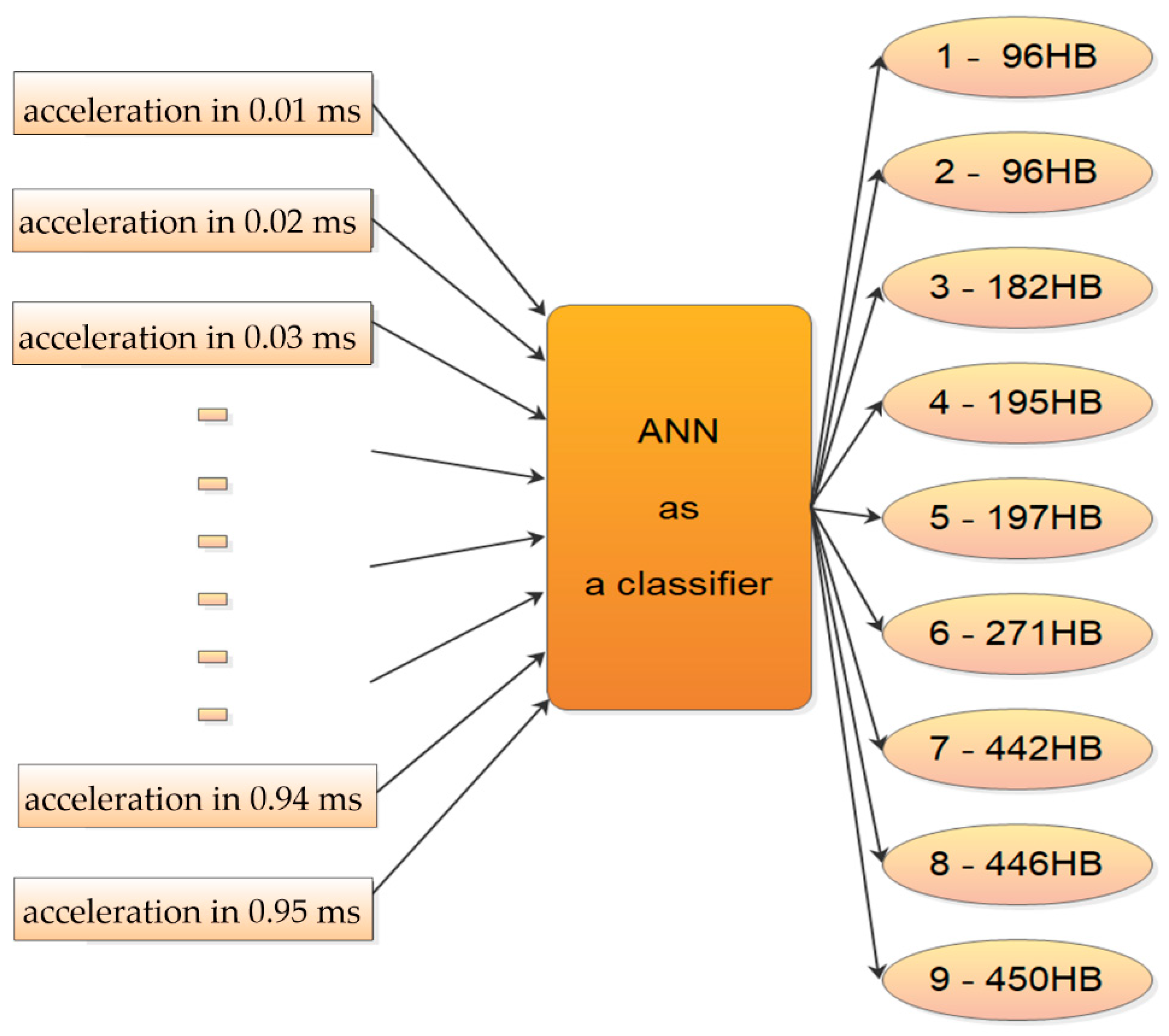


| Steel | C/% | Si/% | Mn/% | Ni/% | Cr/% | Cu/% | Ti/% | V/% | GOST |
|---|---|---|---|---|---|---|---|---|---|
| 08 kp | 0.05–0.11 | 0.03 | 0.25–0.5 | 0.25 | 0.1 | 0.25 | 1050 | ||
| 09G2C | <0.12 | 0.5–0.8 | 1.3–1.7 | 0.3 | 0.3 | 0.3 | 19282 | ||
| 18KhGT | 0.17–0.23 | 0.17–0.37 | 0.8–1.1 | 0.3 | 1.0–1.3 | 0.3 | 0.03–0.09 | 4543 | |
| 20 | 0.17–0.24 | 0.17–0.37 | 0.35–0.65 | 0.25 | 0.25 | 0.25 | 1050 | ||
| 35 | 0.32–.04 | 0.17–0.37 | 0.5–0.8 | 0.25 | 0.25 | 0.25 | 1050 | ||
| 40Kh | 0.36–0.44 | 0.17–0.37 | 0.5–0.8 | 0.3 | 0.8–1.1 | 0.3 | 4543 | ||
| 45 | 0.42–0.5 | 0.17–0.37 | 0.5–0.8 | 0.25 | 0.25 | 0.25 | 1050 | ||
| 50KhFA | 0.46–0.54 | 0.17–0.37 | 0.5–0.8 | 0.25 | 0.8–1.1 | 0.2 | 0.1–0.2 | 14959 | |
| 65G | 0.62–0.7 | 0.17–0.37 | 0.9–1.2 | 0.25 | 0.25 | 0.2 | 14959 |
| Sample Number | Fold 1 | Fold 2 | Fold 3 | Fold 4 | Fold 5 | Fold 6 |
|---|---|---|---|---|---|---|
| 15 | U | T | T | U | T | T |
| 16 | V | T | T | T | T | T |
| 17 | T | U | T | V | U | T |
| 18 | T | V | T | T | T | T |
| 19 | T | T | U | T | V | U |
| 20 | T | T | V | T | T | T |
| 21 | T | T | T | T | T | V |
| Original Class | Predictions | |||||
|---|---|---|---|---|---|---|
| Fold 1 | Fold 2 | Fold 3 | Fold 4 | Fold 5 | Fold 6 | |
| 1 96 HB | 1 96 HB | 1 96 HB | 2 96 HB | 1 96 HB | 1 96 HB | 2 96 HB |
| 2 96 HB | 2 96 HB | 2 96 HB | 2 96 HB | 2 96 HB | 2 96 HB | 2 96 HB |
| 2 96 HB | 2 96 HB | 2 96 HB | 2 96 HB | 2 96 HB | 2 96 HB | 2 96 HB |
| 3 182 HB | 3 182 HB | 3 182 HB | 3 182 HB | 3 182 HB | 3 182 HB | 5 197 HB |
| 4 195 HB | 3 182 HB | 4 195 HB | 5 197 HB | 4 195 HB | 4 195 HB | 5 197 HB |
| 5 197 HB | 5 197 HB | 4 195 HB | 4 195 HB | 5 197 HB | 5 197 HB | 4 195 HB |
| 6 271 HB | 6 271 HB | 6 271 HB | 6 271 HB | 6 271 HB | 6 271 HB | 6 271 HB |
| 7 442 HB | 9 450 HB | 7 442 HB | 7 442 HB | 9 450 HB | 8 446 HB | 8 446 HB |
| 8 446 HB | 8 446 HB | 8 446 HB | 8 446 HB | 8 446 HB | 8 446 HB | 8 446 HB |
| 8 446 HB | 8 446 HB | 8 446 HB | 8 446 HB | 8 446 HB | 8 446 HB | 8 446 HB |
| 9 450 HB | 9 450 HB | 9 450 HB | 9 450 HB | 9 450 HB | 9 450 HB | 9 450 HB |
| Subset | Average Correctness Level in the Steps (in/%) | |||||||
|---|---|---|---|---|---|---|---|---|
| Step 1 | Step 2 | Step 3 | Step 4 | Step 5 | Step 6 | Step 7 | Step 8 | |
| validating | 100.0 | 100.0 | 98.0 | 95.5 | 99.7 | 100.0 | 96.2 | 95.5 |
| all subsets | 100.0 | 100.0 | 100.0 | 100.0 | 100.0 | 100.0 | 97.0 | 95.5 |
| Original Class | Number Correct and Incorrect Classifications | |||||||
|---|---|---|---|---|---|---|---|---|
| Step 1 | Step 2 | Step 3 | Step 4 | Step 5 | Step 6 | Step 7 | Step 8 | |
| 1 96 HB | 30 | 30 | 30 | 30 | 30 | 30 | 30 | 30 |
| 2 96 HB | 54 | 54 | 54 | 54 | 54 | 54 | 54 | 54 |
| 3 182 HB | 42 | 42 | 37; 5 | 42 | 42 | 42 | 42 | 42 |
| 4 195 HB | 42 | 42 | 42 | 42 | 42 | 42 | 42 | 42 |
| 5 197 HB | 36 | 36 | 36 | 30; 6 | 35; 1 | 36 | 36 | 36 |
| 6 271 HB | 42 | 42 | 42 | 42 | 42 | 42 | 42 | 42 |
| 7 442 HB | 42 | 42 | 42 | 42 | 42 | 42 | 29; 13 | 42 |
| 8 446 HB | 72 | 72 | 72 | 72 | 72 | 72 | 72 | 69; 3 |
| 9 450 HB | 42 | 42 | 42 | 42 | 42 | 42 | 41; 1 | 29; 13 |
| End of Assessment at | Class Assessed | Confidence of Assessment | Possible Faults |
|---|---|---|---|
| Step 1 | 1 96 HB | 100.0% | None |
| Step 2 | 2 96 HB | 100.0% | None |
| Step 3 | 3 182 HB | 100.0% | None |
| Step 4 | 4 195 HB | 87.5% | 5 197 HB can be classified as 4 195 HB |
| Step 5 | 5 197 HB | 100.0% | None |
| Step 6 | 6 271 HB | 100.0% | None |
| Step 7 | 7 442 HB | 96.7% | 9 450 HB can be classified as 7 442 HB |
| Step 8 | 8 445 HB | 84.1% | 9 450 HB can be classified as 8 445 HB |
| 9 450 HB | 90.6% | 8 445 HB can be classified as 9 450 HB |
© 2020 by the authors. Licensee MDPI, Basel, Switzerland. This article is an open access article distributed under the terms and conditions of the Creative Commons Attribution (CC BY) license (http://creativecommons.org/licenses/by/4.0/).
Share and Cite
Beskopylny, A.; Lyapin, A.; Anysz, H.; Meskhi, B.; Veremeenko, A.; Mozgovoy, A. Artificial Neural Networks in Classification of Steel Grades Based on Non-Destructive Tests. Materials 2020, 13, 2445. https://doi.org/10.3390/ma13112445
Beskopylny A, Lyapin A, Anysz H, Meskhi B, Veremeenko A, Mozgovoy A. Artificial Neural Networks in Classification of Steel Grades Based on Non-Destructive Tests. Materials. 2020; 13(11):2445. https://doi.org/10.3390/ma13112445
Chicago/Turabian StyleBeskopylny, Alexey, Alexandr Lyapin, Hubert Anysz, Besarion Meskhi, Andrey Veremeenko, and Andrey Mozgovoy. 2020. "Artificial Neural Networks in Classification of Steel Grades Based on Non-Destructive Tests" Materials 13, no. 11: 2445. https://doi.org/10.3390/ma13112445