Nickel-Based Alloy Dry Milling Process Induced Material Softening Effect


Abstract
:1. Introduction
2. Force Model and Milling Temperature Simulation
2.1. Mechanistic Milling Force Model
2.2. Dry Milling Temperature Simulation
3. Experiment Verification
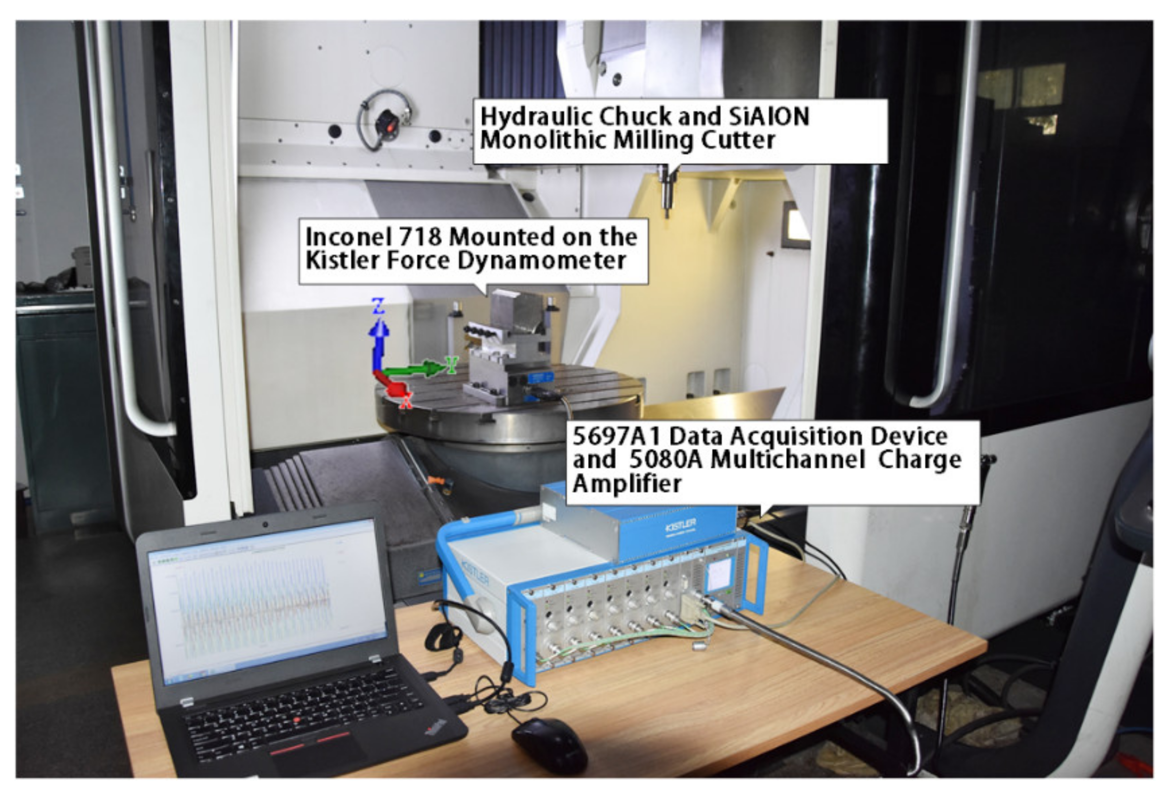
3.1. Experiment Design and Set-Up
3.2. Experiment Results and Discussion
3.3. Tool Wear, Microstructure of Machined Surface, and the Form of Chips Under Different Cutting Parameters
4. Conclusions
- (1)
- The ceramic material SiAlON could withstand the high temperature generated at the shear zone and the accumulated heat under high-speed machining conditions in the dry milling process.
- (2)
- The heat generated in the high-speed milling process could cause a material softening effect on the nickel-based alloy. The average maximum temperature of the shear zone exceeded 1000 °C.
- (3)
- The cutting force turning point was at 527.52 m/min; when the cutting speed exceeded that value, the cutting force began to decrease. When cutting speed continued to increase, the milling force continued to decrease. The milling speed increased the milling temperature to soften the workpiece material. Higher milling speeds could make the milling material removal rate to increase, further making the milling efficiency increase. From the metallographic microscope, the dry milling process had no surface burn on the processed nickel-based alloy surface.
Author Contributions
Funding
Conflicts of Interest
Nomenclature
| a | Cutting depth |
| A | Yield stress under reference deformation conditions (MPa) |
| Aer | Cutting-edge radius |
| Ah | Helical angle |
| Apl | Axial primary land |
| Arf | Radial primary relief angle |
| Art | Radial rake angle (tangential degrees) |
| B | Strain hardening constant (MPa) ε is an equivalent plastic strain |
| c | Feed rate |
| C | Strain rate strengthening coefficient |
| d1~d5 | Failure parameters |
| D | Cutter diameter |
| Dc | Core diameter |
| f(t) | The function of interpolation curve |
| fz | Feed per tooth |
| Fave | Average milling force |
| Fx | Force in the x-direction |
| Fy | Force in the y-direction |
| Fz | Force in the z-direction |
| Average cutting force in x, y, z directions (q = x, y, z) | |
| Cutting force coefficients in x, y, z directions (q = x, y, z) | |
| Edge force which does not depend on the chip thickness (q = x, y, z) | |
| h | Chip thickness |
| Kfc | Cutting force coefficients in the axial direction |
| Kfe | Edge constants in axial direction |
| Krc | Cutting force coefficients in the radial direction |
| Kre | Edge constants in radial direction |
| Ktc | Cutting force coefficients in the tangential direction |
| Kte | Edge constants in tangential direction |
| m | Thermal softening coefficient |
| n | Strain hardening coefficient |
| N | Number of flutes |
| p | Compressive stress |
| q | Mises stress |
| S | Spindle speed |
| r | Force reduction rate |
| t | The average temperature in the milling process |
| T | Current absolute temperature |
| Ti | Initial temperature |
| Tm | Melting temperature |
| Tr | Reference temperature |
| T* | Reference temperature |
| Vc | Cutting speed |
| Wrd | The radial width of cut |
| The equivalent plastic strain of the increment step | |
| Strain rate | |
| Reference strain rate | |
| Equivalent plastic strain | |
| Strain failure value | |
| μ | Friction coefficient |
| τ | Friction stress |
| τ* | Maximum shearing stress |
| σ | Equivalent stress |
| σB | Stefan-Boltzmann constant |
| σn | Normal stress |
| ω | Fracture value |
References
- Suárez, A.; Veiga, F.; Polvorosa, R.; Artaza, T.; Holmbergc, J.; López de Lacalle, L.N.; Wretlande, A. Surface integrity and fatigue of non-conventional machined Alloy 718. J. Manuf. Process. 2019, 48, 44–50. [Google Scholar] [CrossRef]
- Polvorosa, R.; López de Lacalle, L.N.; Egea, A.J.S.; Fernandez, A.; Esparta, M.; Zamakona, I. Cutting edge control by monitoring the tapping torque of new and resharpened tapping tools in Inconel 718. Int. J. Adv. Manuf. Tech. 2020, 106, 3799–3808. [Google Scholar] [CrossRef]
- Yu, T.; Guo, X.; Wang, Z.; Xu, P.F.; Zhao, J. Effects of the ultrasonic vibration field on polishing process of nickel-based alloy Inconel 718. J. Mater. Process. Technol. 2019, 273, 116–228. [Google Scholar] [CrossRef]
- Marques, A.; Suarez, M.P.; Sales, W.F.; Machado, Á.R. Turning of Inconel 718 with whisker-reinforced ceramic tools applying vegetable-based cutting fluid mixed with solid lubricants by MQL. J. Mater. Process. Technol. 2019, 266, 530–543. [Google Scholar] [CrossRef]
- Suárez, A.; López de Lacalle, L.N.; Polvorosa, R.; Veiga, F.; Wretland, A. Effects of high-pressure cooling on the wear patterns on turning inserts used on alloy in 718. Mater. Manuf. Process. 2017, 32, 678–686. [Google Scholar] [CrossRef]
- Thakur, A.; Gangopadhyay, S. State-of-the-art in surface integrity in machining of nickel-based super alloys. Int. J. Mach. Tool. Manuf. 2016, 100, 25–54. [Google Scholar] [CrossRef]
- Polvorosa, R.; Suarez, A.; López de Lacalle, L.N.; Cerrillo, I.; Wretland, A.; Veiga, F. Tool wear on nickel alloys with different coolant pressures: Comparison of alloy 718 and waspaloy. J. Manuf. Process. 2017, 26, 44–56. [Google Scholar] [CrossRef]
- Suárez, A.; Veiga, F.; López de Lacalle, L.N.; Polvorosa, R.; Wretland, A. An investigation of cutting forces and tool wear in turning of Haynes 282. J. Manuf. Process. 2019, 37, 529–540. [Google Scholar] [CrossRef]
- Xavior, M.A.; Manohar, M.; Jeyapandiarajan, P.; Madhukar, P.M. Tool wear assessment during machining of Inconel 718. Proc. Eng. 2017, 174, 1000–1008. [Google Scholar] [CrossRef]
- González, H.; Pereira, O.; Fernández-Valdivielso, A.; López de Lacalle, L.N.; Calleja, A. Comparison of flank super abrasive machining vs. flank milling on inconel® 718 surfaces. Materials 2018, 11, 1638. [Google Scholar] [CrossRef] [Green Version]
- Ezugwu, E.O.; Wang, Z.M.; Machado, A.R. The machinability of nickel-based alloys: A review. J. Mater. Process. Tech. 1998, 86, 1–16. [Google Scholar] [CrossRef]
- Zhang, S.; Li, J.F.; Wang, Y.W. Tool life and cutting forces in end milling Inconel 718 under dry and minimum quantity cooling lubrication cutting conditions. J. Clean. Prod. 2012, 32, 81–87. [Google Scholar] [CrossRef]
- Klocke, F. Manufacturing Processes 1; Springer Press: Berlin, Germany, 2011; pp. 69–72. [Google Scholar]
- Bhatia, S.M.; Pandey, P.C.; Shan, H.S. Thermal cracking of carbide tools during intermittent cutting. Wear 1978, 51, 201–211. [Google Scholar] [CrossRef]
- Habeeb, H.H.; Abou-El-Hossein, K.A.; Bashir, M.; Ghani, J.A.; Kadirgama, K. Investigating of tool wear, tool life and surface roughness when machining of nickel alloy 242 with using of different cutting tools. Asian J. Sci. Res. 2008, 1, 222–230. [Google Scholar] [CrossRef]
- Tan, M.T.; Zhang, Y.Z. Groove wear of tools in nc turning of pure nickel. CIRP. Ann. Manuf. Technol. 1986, 35, 71–74. [Google Scholar] [CrossRef]
- Liao, Y.S.; Lin, H.M.; Wang, J.H. Behaviors of end milling Inconel 718 superalloy by cemented carbide tools. J. Mater. Process. Techol. 2008, 201, 460–465. [Google Scholar] [CrossRef]
- Sun, S.; Brandt, M.; Dargusch, M.S. Thermally enhanced machining of hard-to-machine materials—A review. Int. J. Mach. Tool. Manuf. 2010, 50, 663–680. [Google Scholar] [CrossRef]
- Garcí, A.; Navas, V.; Arriola, I.; Gonzalo, O.; Leunda, J. Mechanisms involved in the improvement of Inconel 718 machinability by laser assisted machining (LAM). Int. J. Mach. Tool. Manuf. 2013, 74, 19–28. [Google Scholar] [CrossRef]
- López de Lacalle, L.N.; Sa´nchez, J.A.; Lamikiz, A.; Celaya, A. Plasma assisted milling of heat-resistant superalloys. J. Manuf. Sci. E. T. ASME 2004, 126, 274–285. [Google Scholar] [CrossRef]
- Leopardi, G.; Tagliaferri, F.; Rüger, C.; Dix, M. Analysis of laser assisted milling (LAM) of Inconel 718 with ceramic tools. Proc. CIRP 2015, 33, 514–519. [Google Scholar] [CrossRef] [Green Version]
- Liu, J. Mechanical property of silicon nitride ceramic structure. J. Foreign Refract. 2011, 7, 50–54. [Google Scholar]
- Grguraš, D.; Kern, M.; Pušavec, F. Suitability of the full body ceramic end milling tools for high speed machining of nickel based alloy Inconel 718. Proc. CIRP 2018, 77, 630–633. [Google Scholar] [CrossRef]
- Davis, D.R.; Landwehr, S.E.; Yeckley, R.L. Monolithic Ceramic End Mill. U.S. Patent 9481041, 11 February 2014. [Google Scholar]
- Altintas, Y. Manufacturing Automation: Metal Cutting Mechanics, Machine Tool Vibrations, and CNC Design, 2nd ed.; Cambridge University Press: Cambridge, UK, 2012. [Google Scholar]
- Fernández-Abia, A.I.; Barreiro, J.; López de Lacalle, L.N.; Pelayo, G.U. A mechanistic model for high speed turning of austenitic stainless steels. Adv. Mater. Res. 2012, 498, 1–6. [Google Scholar] [CrossRef]
- He, A.; Xie, G.; Zhang, H.; Wang, X. A comparative study on Johnson–Cook, modified Johnson–Cook and Arrhenius-type constitutive models to predict the high temperature flow stress in 20CrMo alloy steel. Mater. Des. 2013, 52, 677–685. [Google Scholar] [CrossRef]
- Johnson, G.R.; Cook, W.H. Fracture characteristics of three metals subjected to various strains, strain rates, temperatures and pressures. Eng. Fract. Mech. 1985, 21, 31–48. [Google Scholar] [CrossRef]
- Chen, B.; Liu, W.; Luo, M.; Zhang, X. Reverse Identification of John-Cook constitutive parameters of superalloy based on orthogonal cutting. J. Mech. Eng. 2019, 55, 217–224. [Google Scholar] [CrossRef] [Green Version]
- Cercignani, C. The Boltzmann Equation and Its Applications; Springer: New York, NY, USA, 1988; pp. 40–103. [Google Scholar]


| Number | 0 | 1 | 2 | 3 | 4 | 5 | 6 | 7 | 8 | 9 |
|---|---|---|---|---|---|---|---|---|---|---|
| Feed per tooth (mm/tooth) | 0.015 | 0.02 | 0.025 | 0.03 | 0.035 | 0.04 | 0.045 | 0.05 | 0.055 | 0.06 |
| Ktc | Kte | Krc | Kre | Kfc | Kfe |
|---|---|---|---|---|---|
| −538.26 | −200.89 | −5004.21 | 178.32 | 12973.39 | 274.29 |
| Parameters | Value |
|---|---|
| Feed per tooth/fz | 0.03 mm/tooth |
| Radial width of cut/Wrd | 5 mm |
| Initial temperature/Ti | 20 °C |
| Cutter diameter/D | 12 mm |
| Core diameter/Dc | 9.02 mm |
| Number of flutes/N | 6 |
| Radial rake (tangential degrees)/Art | −2° |
| Helical angle/Ah | 40° |
| Cutting-edge radius/Aer | 2 |
| Radial primary relief angle/Arf | 8° |
| Axial primary land/Apl | 0.71 mm |
| Cutting speed/VC | 300 m/min, 400 m/min, 500 m/min, 600 m/min, 700 m/min |
| Parameters | d1 | d2 | d3 | d4 | d5 |
|---|---|---|---|---|---|
| Value | 0.11 | 0.75 | −1.45 | 0.04 | 0.89 |
| Parameters | A (MPa) | B (MPa) | C | n | m | |
|---|---|---|---|---|---|---|
| Value | 1241 | 622 | 0.0134 | 0.6522 | 1.3 | 1 |
| Parameters | Density (g/cm3) | Melting Point (°C) | Thermal Conductivity | Specific Heat Capacity | Poisson Rate |
|---|---|---|---|---|---|
| Value | 8.24 | 1260–1360 | 14.7 (100 °C) | 435 | 0.3 |
© 2020 by the authors. Licensee MDPI, Basel, Switzerland. This article is an open access article distributed under the terms and conditions of the Creative Commons Attribution (CC BY) license (http://creativecommons.org/licenses/by/4.0/).
Share and Cite
Zha, J.; Yuan, Z.; Zhang, H.; Li, Y.; Chen, Y. Nickel-Based Alloy Dry Milling Process Induced Material Softening Effect. Materials 2020, 13, 3758. https://doi.org/10.3390/ma13173758
Zha J, Yuan Z, Zhang H, Li Y, Chen Y. Nickel-Based Alloy Dry Milling Process Induced Material Softening Effect. Materials. 2020; 13(17):3758. https://doi.org/10.3390/ma13173758
Chicago/Turabian StyleZha, Jun, Zelong Yuan, Hangcheng Zhang, Yipeng Li, and Yaolong Chen. 2020. "Nickel-Based Alloy Dry Milling Process Induced Material Softening Effect" Materials 13, no. 17: 3758. https://doi.org/10.3390/ma13173758
APA StyleZha, J., Yuan, Z., Zhang, H., Li, Y., & Chen, Y. (2020). Nickel-Based Alloy Dry Milling Process Induced Material Softening Effect. Materials, 13(17), 3758. https://doi.org/10.3390/ma13173758