High Precision Detection Method for Delamination Defects in Carbon Fiber Composite Laminates Based on Ultrasonic Technique and Signal Correlation Algorithm

 , ,
, ,
Abstract
:1. Introduction
2. Proposed Method Based on Signal Correlation
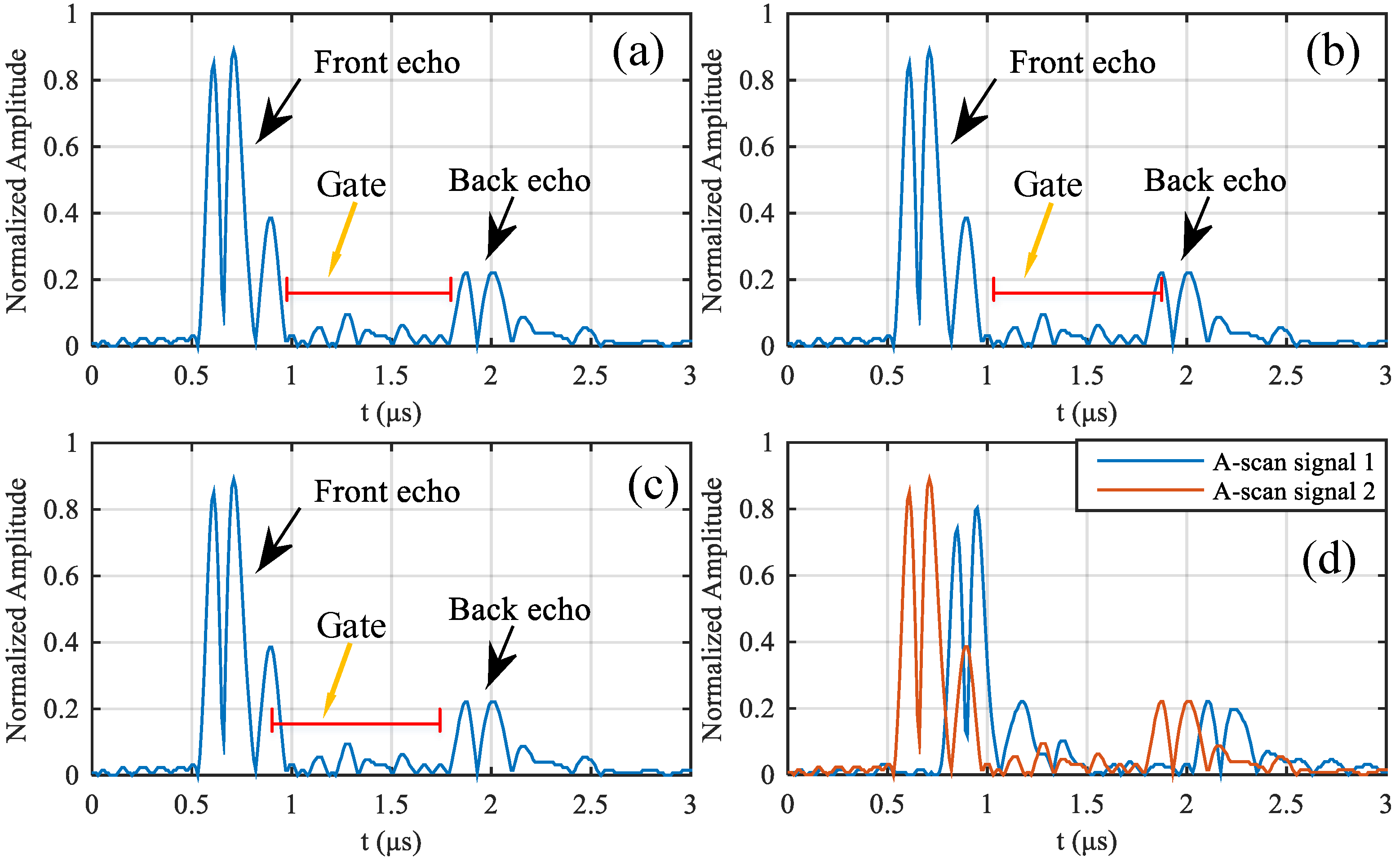
2.1. Classical Ultrasonic C-Scan Method
2.2. A-Scan Signal Correlation Algorithm
2.3. Overview of The Method
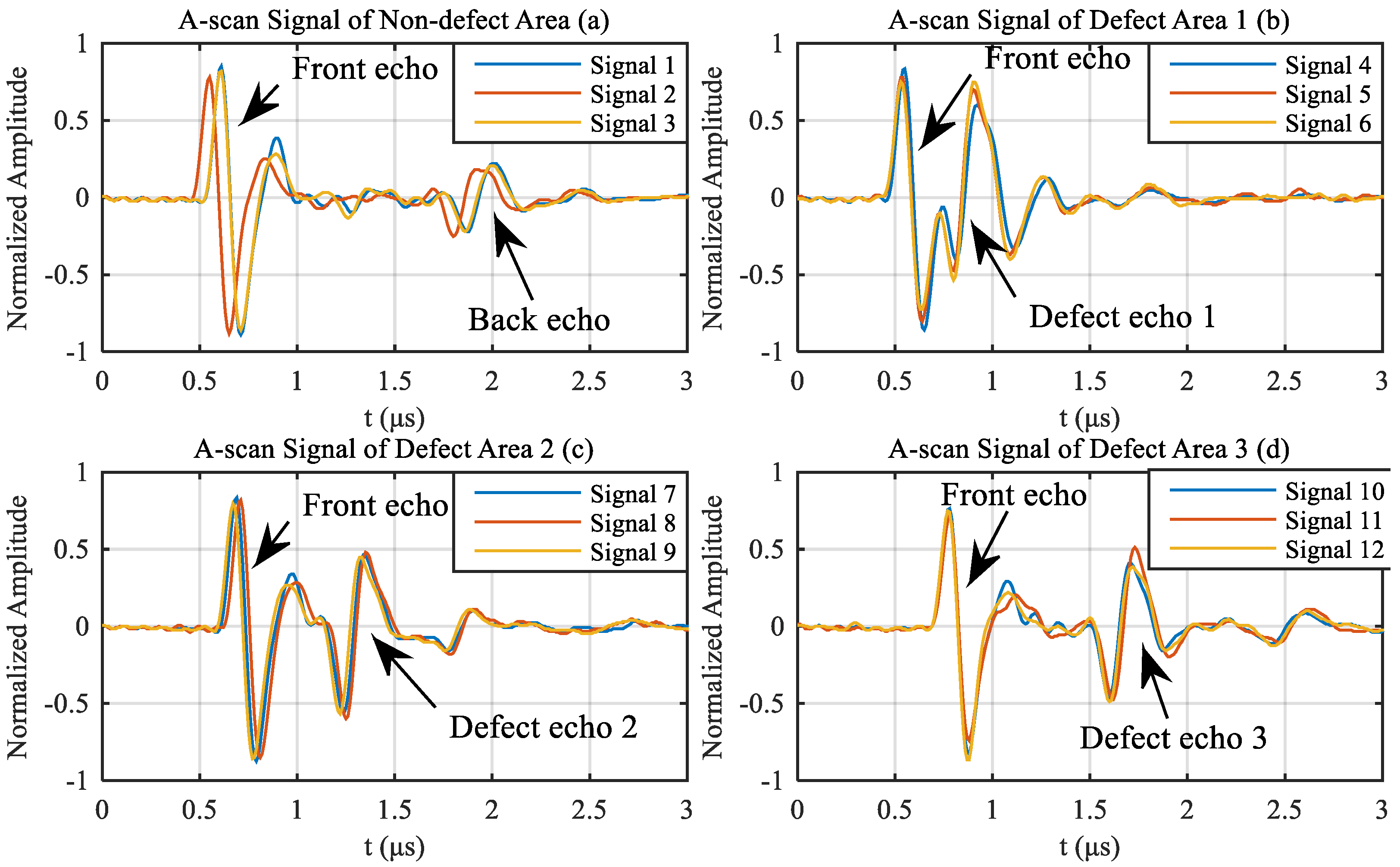
- Step 1: Acquire standard A-scan signals from non-defect area. In order to reduce the influence of random errors, the number of signals should be greater than 10.
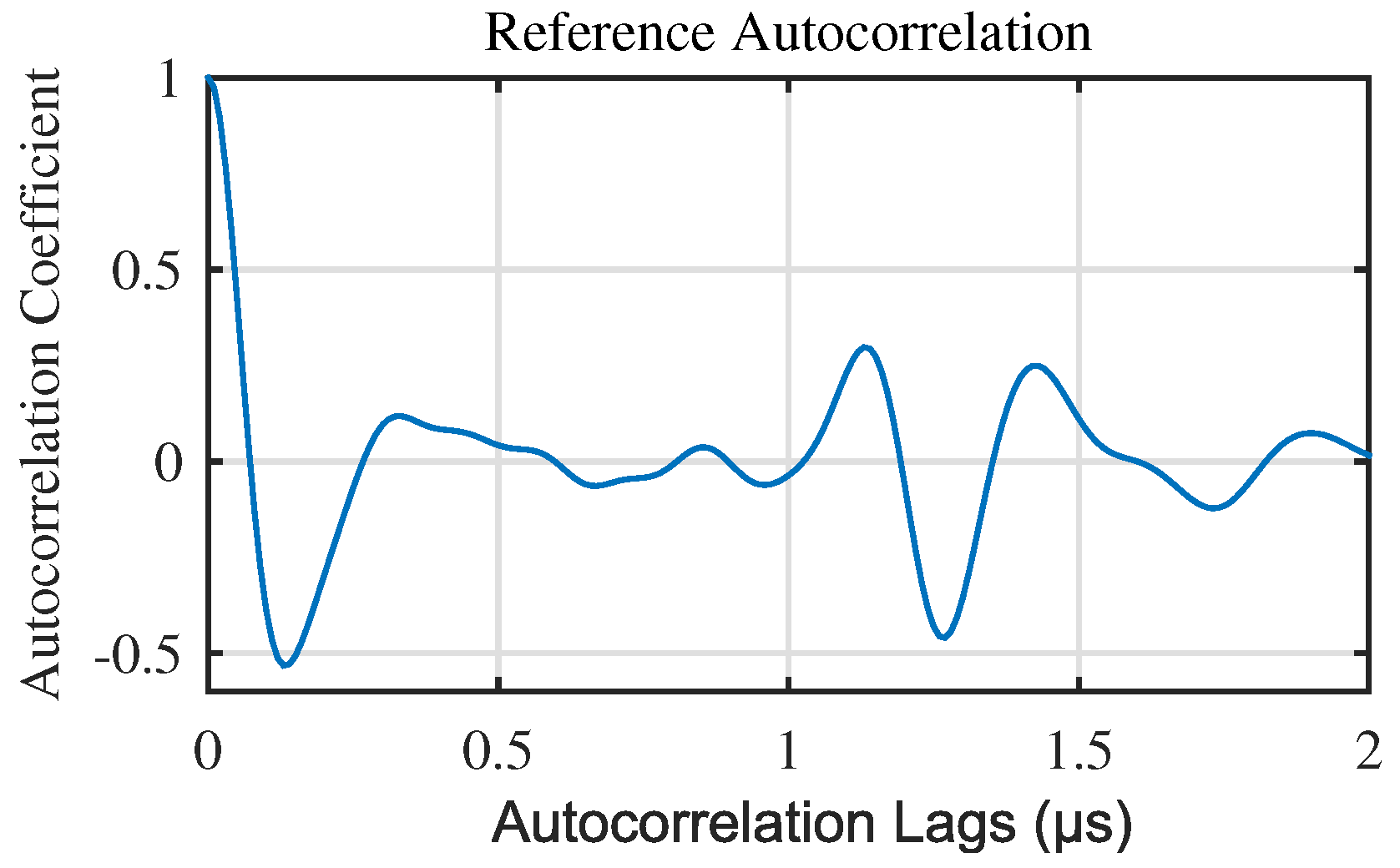
- Step 2: Calculate autocorrelation from above standard A-scan signals and generate reference autocorrelation, which is detailed in Section 2.4.
- Step 3: Ultrasonic scan of all areas of the object to obtain A-scan signals, during which the parameters such as the distance between the ultrasonic transducer and the object to be measured, the ultrasonic excitation pulse voltage, the ultrasonic echo signal sampling rate, and the signal gain should be set to be consistent with Step 1.
- Step 4: Calculate autocorrelation for all A-scan signals, and classify signals from defect and non-defect, which is detailed in Section 2.5.
- Step 5: Generate the defect image by Euclidean distance rather than the amplitude of the defect echo used in traditional ultrasonic C-scan. To improve visibility, we use pseudo-color coding to convert gray images into color images.
- Step 6: Calculate the defect depth of the A-scan signals of the classified defect area, which is detailed in Section 2.6.
2.4. Generate Reference Signal
2.5. Classification of Defective and Non-Defective Signals
2.6. Calculation of Defect Depth
- Step 1: Intercept the first peak of the reference autocorrelation, record as .
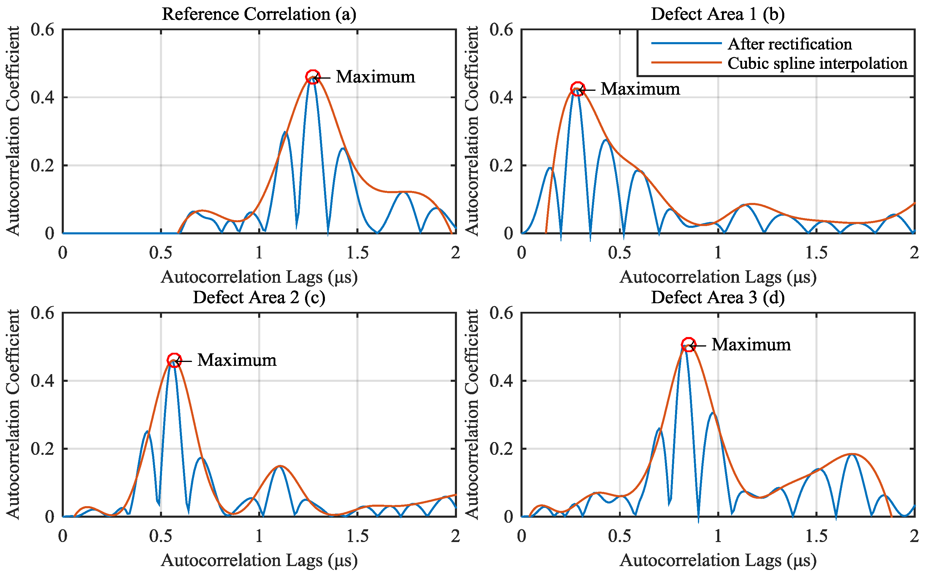
- Step 2: Calculate the defect peak by the follow function.where is the defect peak, is the autocorrelation of defect signal, is the first peak of the reference autocorrelation.
- Step 3: Use median filter to smooth the curve of defect peak, and get .
- Step 4: Find the peaks of , as , where i is the order number of peaks. Use cubic spline interpolation to interpolate these peaks, record as . Set the interval as one tenth of the original signal interval.
- Step 5: Find the maximum value of , record as . The corresponding to the maximum value is the required sound path. Finally, the defect depth can be calculated from .
2.7. Advantages of Proposed Algorithm over Traditional Ultrasonic C-Scan Method
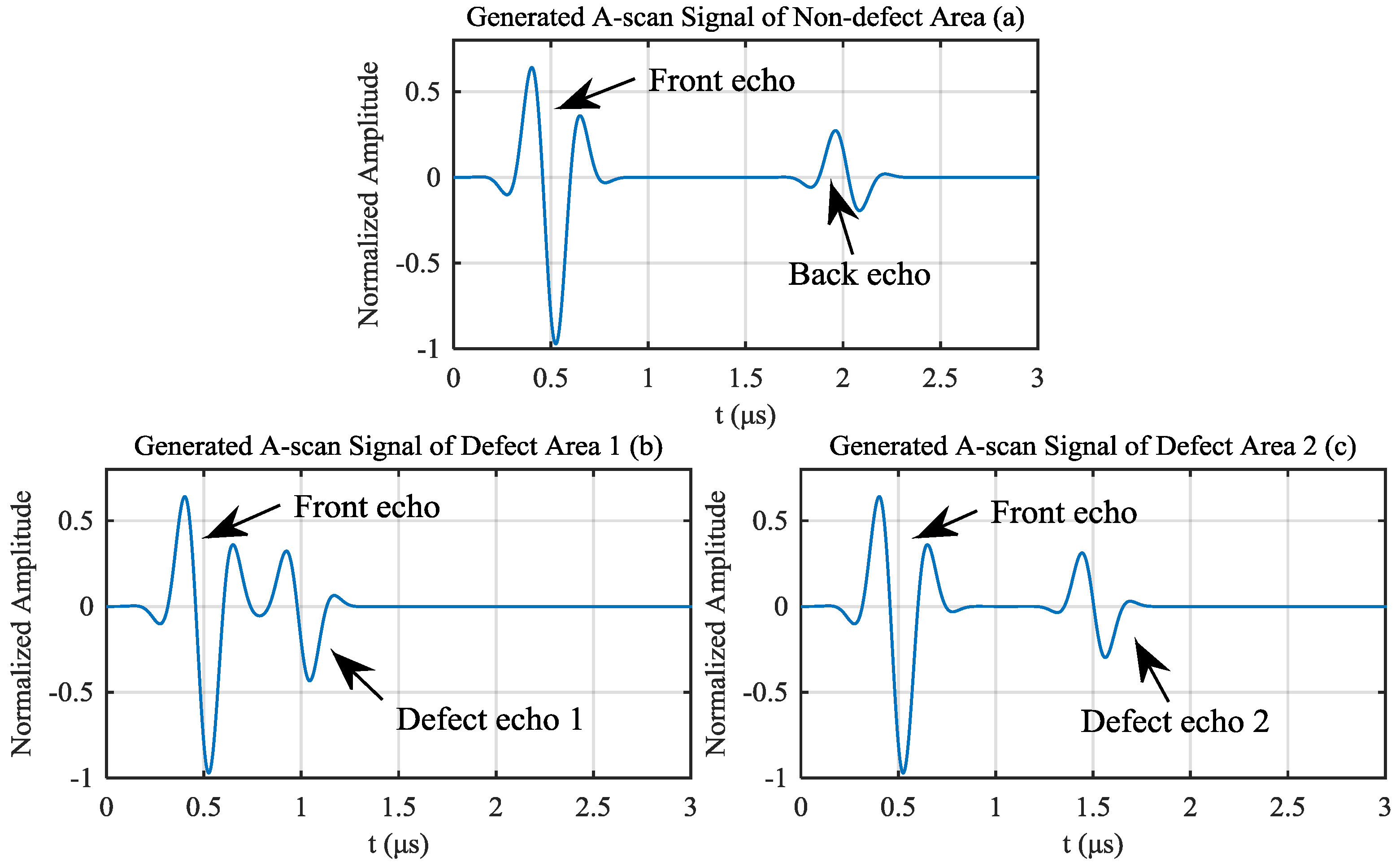
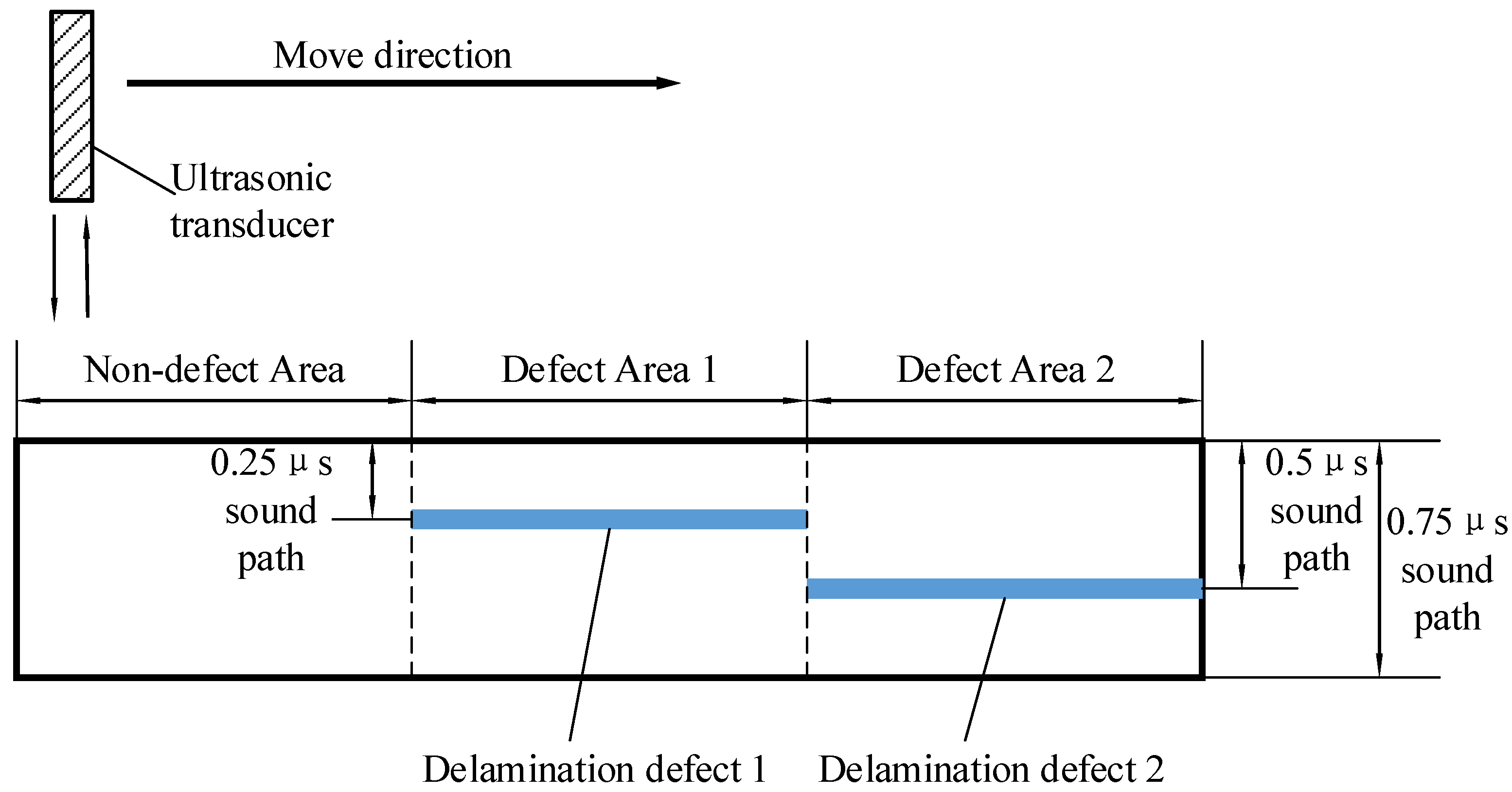
3. Simulation Based on Artificial Echo Signals
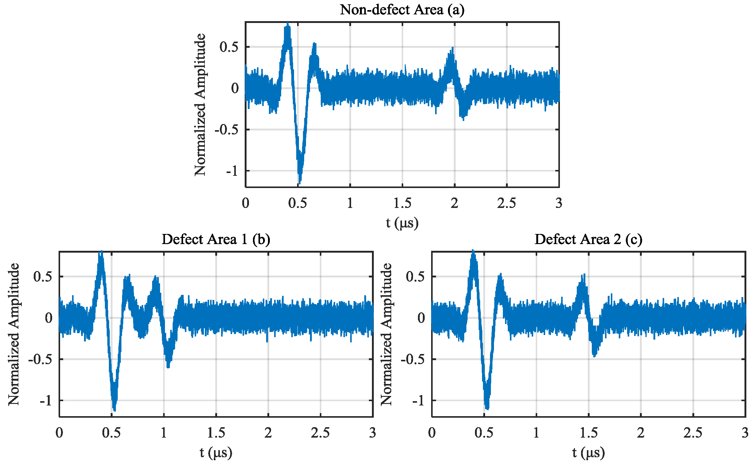
4. Experimental Test Result And Discussion
4.1. Signal Filtering
4.2. Generating Reference Signal
4.3. Signal Classification And Results
4.4. Defect Depth Calculation And Comparing
4.5. Defect Imaging And Comparing
4.6. Comparison of Phased Array C-Scan, Conventional Ultrasonic C-Scan and Proposed Algorithm
- (1)
- The phased array ultrasonic C-scan has higher detection accuracy and speed than conventional ultrasonic C-scan and the proposed algorithm.
- (2)
- The proposed algorithm can avoid signal peak tracking and complex gate setting, which are necessary when using phased array ultrasonic C-scan and conventional ultrasonic C-scan. The proposed algorithm needs less prior knowledge, more convenient for operators to measure objects and more suitable for automated testing.
- (3)
- Compared with conventional ultrasonic C-scan method, the proposed algorithm can calculated depth and size of the near surface defect better.
- (4)
- In addition, we found in actual measurement that the proposed algorithm is more sensitive to the surface of the object. As a result, when the surface of the object to be tested is uniform, the proposed algorithm performs better.
5. Conclusions
- (1)
- By using signal autocorrelation instead of the original ultrasonic pulse-echo signal, some problems can be avoided, such as complex gate setting and signal peak tracking because of the slight change in the distance between the ultrasonic transducer and the laminate which can lead to signal peak time shift.
- (2)
- The proposed algorithm only requires a small amount of reference signals in non-defect areas, without prior knowledge and adjustment of parameters such as gates and thresholds.
- (3)
- The proposed algorithm can detect the depth and size of defects with high precision. The defect size error is less than 4%, and the defect depth error is less than 3%. Provides a high-precision ultrasonic detection and signal processing method.
- (4)
- The proposed algorithm provides a new idea and direction for ultrasonic visual testing and can be widely used in automated ultrasonic testing.
Author Contributions
Funding
Conflicts of Interest
References
- Mohammadkhani, R.; Fragonara, L.Z.; Janardhan, P.M.; Petrunin, I.; Tsourdos, A.; Gray, I. Ultrasonic Phased Array Imaging Technology for the Inspection of Aerospace Composite Structures. In Proceedings of the 2019 IEEE 5th International Workshop on Metrology for AeroSpace (MetroAeroSpace), Torino, Italy, 19–21 June 2019; IEEE: Piscataway, NJ, USA, 2019; pp. 203–208. [Google Scholar]
- Zhang, X.H.; Yang, H.; Zhang, H.; Wang, C.Y. A carbon fiber reinforced nylon 6 (CFRPA6) composite specialized for military field cooking task. Applied Mechanics and Materials. Trans. Tech. Publ. 2012, 224, 199–203. [Google Scholar]
- Lee, J.C.; Park, D.H.; Jung, H.S.; Lee, S.H.; Jeong, W.Y.; Kim, K.Y.; Lim, D.Y. Design for Carbon Fiber Lamination of PMI Foam Cored CFRP Sandwich Composite Applied to Automotive Rear Spoiler. Fibers Polym. 2020, 21, 156–161. [Google Scholar] [CrossRef]
- Maierhofer, C.; Myrach, P.; Reischel, M.; Steinfurth, H.; Röllig, M.; Kunert, M. Characterizing damage in CFRP structures using flash thermography in reflection and transmission configurations. Compos. Part B Eng. 2014, 57, 35–46. [Google Scholar] [CrossRef]
- Isbilir, O.; Ghassemieh, E. Numerical investigation of the effects of drill geometry on drilling induced delamination of carbon fiber reinforced composites. Compos. Struct. 2013, 105, 126–133. [Google Scholar] [CrossRef]
- Meola, C.; Boccardi, S.; Carlomagno, G.; Boffa, N.; Monaco, E.; Ricci, F. Nondestructive evaluation of carbon fibre reinforced composites with infrared thermography and ultrasonics. Compos. Struct. 2015, 134, 845–853. [Google Scholar] [CrossRef]
- Caminero, M.; García-Moreno, I.; Rodríguez, G.; Chacón, J. Internal damage evaluation of composite structures using phased array ultrasonic technique: Impact damage assessment in CFRP and 3D printed reinforced composites. Compos. Part B Eng. 2019, 165, 131–142. [Google Scholar] [CrossRef]
- Garcia, C.; Trendafilova, I. Triboelectric sensor as a dual system for impact monitoring and prediction of the damage in composite structures. Nano Energy 2019, 60, 527–535. [Google Scholar] [CrossRef] [Green Version]
- Blandford, B.M.; Jack, D.A. High resolution depth and area measurements of low velocity impact damage in carbon fiber laminates via an ultrasonic technique. Compos. Part B Eng. 2020, 188, 107843. [Google Scholar] [CrossRef]
- Liu, Y.; Li, X.; Zhang, G.; Zhang, S.; Jeong, H. Characterizing Microstructural Evolution of TP304 Stainless Steel Using a Pulse-Echo Nonlinear Method. Materials 2020, 13, 1395. [Google Scholar] [CrossRef] [Green Version]
- Ryuzono, K.; Yashiro, S.; Nagai, H.; Toyama, N. Topology Optimization-Based Damage Identification Using Visualized Ultrasonic Wave Propagation. Materials 2020, 13, 33. [Google Scholar] [CrossRef] [Green Version]
- Slonski, M.; Schabowicz, K.; Krawczyk, E. Detection of Flaws in Concrete Using Ultrasonic Tomography and Convolutional Neural Networks. Materials 2020, 13, 1557. [Google Scholar] [CrossRef] [PubMed] [Green Version]
- Naqiuddin, M.M.; Leong, M.S.; Hee, L.; Azrieasrie, M. Ultrasonic signal processing techniques for Pipeline: A review. MATEC Web of Conferences. EDP Sci. 2019, 255, 06006. [Google Scholar]
- Tiwari, K.A.; Raisutis, R.; Samaitis, V. Hybrid signal processing technique to improve the defect estimation in ultrasonic non-destructive testing of composite structures. Sensors 2017, 17, 2858. [Google Scholar] [CrossRef] [Green Version]
- Wang, B.; Saniie, J. A High Performance Ultrasonic System for Flaw Detection. In Proceedings of the 2019 IEEE International Ultrasonics Symposium (IUS), Glasgow, UK, 6–9 October 2019; IEEE: Piscataway, NJ, USA, 2019; pp. 840–843. [Google Scholar]
- Pedram, S.K.; Mudge, P.; Gan, T.H. Enhancement of ultrasonic guided wave signals using a split-spectrum processing method. Appl. Sci. 2018, 8, 1815. [Google Scholar] [CrossRef] [Green Version]
- Garcia Marquez, F.P.; Gomez Munoz, C.Q. A New Approach for Fault Detection, Location and Diagnosis by Ultrasonic Testing. Energies 2020, 13, 1192. [Google Scholar] [CrossRef] [Green Version]
- Zhang, M.; Li, M.; Zhang, J.; Liu, L.; Li, H. Onset detection of ultrasonic signals for the testing of concrete foundation piles by coupled continuous wavelet transform and machine learning algorithms. Adv. Eng. Inform. 2020, 43, 101034. [Google Scholar] [CrossRef]
- Xue, R.; Wang, X.; Yang, Q.; Dong, F.; Zhang, Y.; Cao, J.; Song, G. Grain size characterization of aluminum based on ensemble empirical mode decomposition using a laser ultrasonic technique. Appl. Acoust. 2019, 156, 378–386. [Google Scholar] [CrossRef]
- Gao, F.; Wei, J.X.; Di, B.R. Ultrasonic attenuation estimation based on time-frequency analysis. Appl. Geophys. 2019. [Google Scholar] [CrossRef]
- Cai, H.; Xu, C.; Zhou, S.; Yan, H.; Yang, L. Study on the thick-walled pipe ultrasonic signal enhancement of modified S-transform and singular value decomposition. Math. Probl. Eng. 2015, 2015, 312620. [Google Scholar] [CrossRef]
- Rodríguez, A.; Miralles, R.; Bosch, I.; Vergara, L. New analysis and extensions of split-spectrum processing algorithms. NDT & E Int. 2012, 45, 141–147. [Google Scholar]
- Bouden, T.; Djerfi, F.; Nibouche, M. Adaptive split spectrum processing for ultrasonic signal in the pulse echo test. Russ. J. Nondestruct. Test. 2015, 51, 245–257. [Google Scholar] [CrossRef]
- Praveen, A.; Vijayarekha, K.; Abraham, S.T.; Venkatraman, B. Signal quality enhancement using higher order wavelets for ultrasonic TOFD signals from austenitic stainless steel welds. Ultrasonics 2013, 53, 1288–1292. [Google Scholar] [CrossRef] [PubMed]
- Mohammadkhani, R.; Zanotti Fragonara, L.; Padiyar, M.J.; Petrunin, I.; Raposo, J.; Tsourdos, A.; Gray, I. Improving Depth Resolution of Ultrasonic Phased Array Imaging to Inspect Aerospace Composite Structures. Sensors 2020, 20, 559. [Google Scholar] [CrossRef] [PubMed] [Green Version]
- Luo, Y.; Xue, W.; Yu, Y. Ultrasonic Signal Denoising Based on a New Wavelet Thresholding Function. In Proceedings of the 2018 37th Chinese Control Conference (CCC), Wuhan, China, 25–27 July 2018; IEEE: Piscataway, NJ, USA, 2018; pp. 4363–4367. [Google Scholar]
- Lu, Y.; Oruklu, E.; Saniie, J. Application of Hilbert-Huang transform for ultrasonic nondestructive evaluation. In Proceedings of the 2008 IEEE Ultrasonics Symposium, Beijing, China, 2–5 November 2008; IEEE: Piscataway, NJ, USA, 2008; pp. 1499–1502. [Google Scholar]
- Sharma, G.K.; Kumar, A.; Jayakumar, T.; Rao, B.P.; Mariyappa, N. Ensemble Empirical Mode Decomposition based methodology for ultrasonic testing of coarse grain austenitic stainless steels. Ultrasonics 2015, 57, 167–178. [Google Scholar] [CrossRef] [PubMed]
- Ali, M.G.; Warraich, S.A.; Khan, T.M. Evaluation of the aging effect on mild steel (E 6013) welded areas using Hilbert Huang Transform on UT signals. In Proceedings of the 2016 International Conference on Emerging Technologies (ICET), Islamabad, Pakistan, 18–19 October 2016; IEEE: Piscataway, NJ, USA, 2016; pp. 1–5. [Google Scholar]
- Shi, Z.; Liu, L.; Peng, M.; Liu, C.; Tao, F.; Liu, C. Non-destructive testing of full-length bonded rock bolts based on HHT signal analysis. J. Appl. Geophys. 2018, 151, 47–65. [Google Scholar] [CrossRef]
- Malik, M.A.; Saniie, J. S-transform applied to ultrasonic nondestructive testing. In Proceedings of the 2008 IEEE Ultrasonics Symposium, Beijing, China, 2–5 November 2008; IEEE: Piscataway, NJ, USA, 2008; pp. 184–187. [Google Scholar]
- Benammar, A.; Drai, R.; Guessoum, A. Ultrasonic flaw detection using threshold modified S-transform. Ultrasonics 2014, 54, 676–683. [Google Scholar] [CrossRef]
- Xu, J.; Wei, H. Ultrasonic testing analysis of concrete structure based on S transform. Shock. Vib. 2019, 2019. [Google Scholar] [CrossRef]
- Zhu, Y.; Xu, C.; Xiao, D. Denoising Ultrasonic Echo Signals with Generalized S Transform and Singular Value Decomposition. Trait. Signal 2019, 36, 139–145. [Google Scholar] [CrossRef]
- Song, Y.; Kube, C.M.; Zhang, J.; Li, X. Higher-order spatial correlation coefficients of ultrasonic backscattering signals using partial cross-correlation analysis. J. Acoust. Soc. Am. 2020, 147, 757–768. [Google Scholar] [CrossRef]
- Zhang, H.; Shao, M.; Fan, G.; Zhang, H.; Zhu, W.; Zhu, Q. Phase Coherence Imaging for Near-Surface Defects in Rails Using Cross-Correlation of Ultrasonic Diffuse Fields. Metals 2019, 9, 868. [Google Scholar] [CrossRef] [Green Version]
- Zhang, H.; Zhang, J.; Fan, G.; Zhang, H.; Zhu, W.; Zhu, Q.; Zheng, R. The Auto-Correlation of Ultrasonic Lamb Wave Phased Array Data for Damage Detection. Metals 2019, 9, 666. [Google Scholar] [CrossRef] [Green Version]
- Kawamura, Y.; Tsurushima, M.; Mizutani, K.; Ujihira, M.; Aoshima, N.; Kuraoka, S. Ultrasonic measurement system for detecting penetration of boulders by autocorrelation analysis. Jpn. J. Appl. Phys. 2005, 44, 4364. [Google Scholar] [CrossRef]
- Liang, W.; Chen, L.; Zhou, F.x.; Ge, Z.H.; Ding, G. Maximum fraction cross-correlation spectrum for time of arrival estimation of ultrasonic echoes. Russ. J. Nondestruct. Test. 2015, 51, 120–130. [Google Scholar] [CrossRef]
- Luppescu, G.C.; Dawson, A.J.; Michaels, J.E. Dispersive matched filtering of ultrasonic guided waves for improved sparse array damage localization. In AIP Conference Proceedings; AIP Publishing LLC: Melville, NY, USA, 2016; Volume 1706, p. 030008. [Google Scholar]
- Li, S.; Poudel, A.; Chu, T.P. Ultrasonic defect mapping using signal correlation for nondestructive evaluation (NDE). Res. Nondestruct. Eval. 2015, 26, 90–106. [Google Scholar] [CrossRef]
- Hasiotis, T.; Badogiannis, E.; Tsouvalis, N.G. Application of ultrasonic C-scan techniques for tracing defects in laminated composite materials. Stroj. -Vestn. -J. Mech. Eng. 2011, 57, 192–203. [Google Scholar] [CrossRef]
- Wronkowicz, A.; Dragan, K.; Lis, K. Assessment of uncertainty in damage evaluation by ultrasonic testing of composite structures. Compos. Struct. 2018, 203, 71–84. [Google Scholar] [CrossRef]
- Demirli, R. Model Based Estimation of Ultrasonic Echoes: Analysis, Algorithms, and Applications. Ph.D. Thesis, Illinois Institute of Technology, Chicago, IL, USA, 2001. [Google Scholar]


| Sample | Non-Defect Area | Defect Area 1 | Defect Area 2 |
|---|---|---|---|
| 1 | 0.3733 | 7.1439 | 7.1929 |
| 2 | 0.4343 | 7.1246 | 7.3927 |
| 3 | 0.5421 | 7.1526 | 7.4258 |
| 4 | 0.4091 | 7.3631 | 7.3605 |
| 5 | 0.4995 | 7.1424 | 7.3247 |
| Sample | Defect Area 1 (Depth 0.25) | Defect Area 2 (Depth 0.5) | ||
|---|---|---|---|---|
| Depth | Error (%) | Depth | Error (%) | |
| 1 | 0.2568 | 2.72 | 0.5037 | 0.74 |
| 2 | 0.2579 | 3.14 | 0.5087 | 1.73 |
| 3 | 0.2573 | 2.92 | 0.5104 | 2.08 |
| 4 | 0.2570 | 2.80 | 0.5085 | 1.70 |
| 5 | 0.2572 | 2.88 | 0.5032 | 0.64 |
| Sample | Non-Defect Area | Defect Area 1 | Defect Area 2 | Defect Area 3 |
|---|---|---|---|---|
| 1 | 0.3337 | 2.5523 | 2.5838 | 2.5079 |
| 2 | 0.3790 | 2.5026 | 2.5202 | 2.4704 |
| 3 | 0.2483 | 2.3818 | 2.4829 | 2.4303 |
| 4 | 0.2769 | 2.2894 | 2.6116 | 2.5084 |
| 5 | 0.3649 | 2.2639 | 2.6179 | 2.5416 |
| 6 | 0.3048 | 2.2975 | 2.6149 | 2.5653 |
| 7 | 0.1855 | 2.3653 | 2.5982 | 2.5945 |
| 8 | 0.4699 | 2.4036 | 2.5936 | 2.4551 |
| 9 | 0.5050 | 2.4889 | 2.5563 | 2.5349 |
| 10 | 0.3381 | 2.5701 | 2.6070 | 2.6140 |
| Sample | Defect Area 1 (0.41 mm Depth) | Defect Area 2 (0.86 mm Depth) | Defect Area 3 (1.32 mm Depth) | |||
|---|---|---|---|---|---|---|
| Depth (mm) | Error (%) | Depth (mm) | Error (%) | Depth (mm) | Error (%) | |
| 1 | 0.4401 | 7.3400 | 0.8833 | 2.7117 | 1.3312 | 0.8519 |
| 2 | 0.4401 | 7.3400 | 0.8802 | 2.3474 | 1.3359 | 1.2078 |
| 3 | 0.4291 | 4.6660 | 0.8708 | 1.2548 | 1.3422 | 1.6824 |
| 4 | 0.4072 | 0.6819 | 0.8661 | 0.7084 | 1.3438 | 1.8011 |
| 5 | 0.3962 | 3.3558 | 0.8661 | 0.7084 | 1.3485 | 2.1570 |
| 6 | 0.4150 | 1.2281 | 0.8677 | 0.8905 | 1.3438 | 1.8011 |
| 7 | 0.4197 | 2.3741 | 0.8692 | 1.0726 | 1.3281 | 0.6146 |
| 8 | 0.4276 | 4.2840 | 0.8708 | 1.2548 | 1.3375 | 1.3265 |
| 9 | 0.4150 | 1.2281 | 0.8739 | 1.6190 | 1.3406 | 1.5638 |
| 10 | 0.4135 | 0.8461 | 0.8645 | 0.5263 | 1.3485 | 2.1570 |
| Average | 0.4204 | 2.5269 | 0.8713 | 1.3094 | 1.3400 | 1.5163 |
| Measurement Method | Defect Area 1 | Defect Area 2 | Defect Area 3 | |
|---|---|---|---|---|
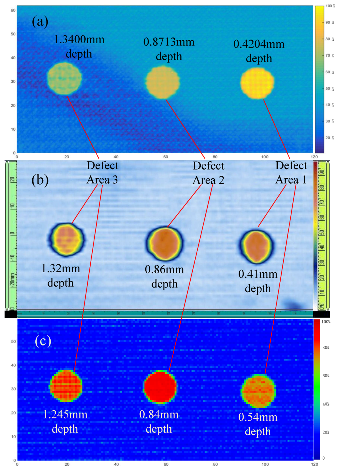
| Olympus OmniScan MX2 (mm) | 0.41 | 0.86 | 1.32 | |
| Conventional ultrasonic C-scan | Depth (mm) | 0.54 | 0.84 | 1.245 |
| Error (%) | 31.707 | 2.3256 | 5.6818 | |
| Proposed algorithm | Depth (mm) | 0.4204 | 0.8713 | 1.3400 |
| Error (%) | 2.5269 | 1.3094 | 1.5163 | |
| Detect Items | OmniScan MX2 | Proposed Algorithm | Error | Conventional C-Scan | Error | |
|---|---|---|---|---|---|---|
| Defect Area 3 | Length | 12.90 | 13.125 | 1.744% | 13.5 | 4.444% |
| Width | 12.55 | 12.75 | 1.594% | 12.75 | 1.594% | |
| Defect Area 2 | Length | 13.00 | 12.75 | 1.923% | 13.125 | 1.154% |
| Width | 12.95 | 13.125 | 1.351% | 13.125 | 1.351% | |
| Defect Area 1 | Length | 11.90 | 12.375 | 3.992% | 12.75 | 7.143% |
| Width | 12.35 | 12.75 | 3.239% | 12.75 | 6.275% | |
© 2020 by the authors. Licensee MDPI, Basel, Switzerland. This article is an open access article distributed under the terms and conditions of the Creative Commons Attribution (CC BY) license (http://creativecommons.org/licenses/by/4.0/).
Share and Cite
Ma, M.; Cao, H.; Jiang, M.; Sun, L.; Zhang, L.; Zhang, F.; Sui, Q.; Tian, A.; Liang, J.; Jia, L. High Precision Detection Method for Delamination Defects in Carbon Fiber Composite Laminates Based on Ultrasonic Technique and Signal Correlation Algorithm. Materials 2020, 13, 3840. https://doi.org/10.3390/ma13173840
Ma M, Cao H, Jiang M, Sun L, Zhang L, Zhang F, Sui Q, Tian A, Liang J, Jia L. High Precision Detection Method for Delamination Defects in Carbon Fiber Composite Laminates Based on Ultrasonic Technique and Signal Correlation Algorithm. Materials. 2020; 13(17):3840. https://doi.org/10.3390/ma13173840
Chicago/Turabian StyleMa, Mengyuan, Hongyi Cao, Mingshun Jiang, Lin Sun, Lei Zhang, Faye Zhang, Qingmei Sui, Aiqin Tian, Jianying Liang, and Lei Jia. 2020. "High Precision Detection Method for Delamination Defects in Carbon Fiber Composite Laminates Based on Ultrasonic Technique and Signal Correlation Algorithm" Materials 13, no. 17: 3840. https://doi.org/10.3390/ma13173840