Shear Wave Splitting and Polarization in Anisotropic Fluid-Infiltrating Porous Media: A Numerical Study


Abstract
1. Introduction
2. Mathematical Model
2.1. Governing Equations
2.2. Constitutive Laws
2.2.1. Effective Stress Law for Anisotropic Elasticity
2.2.2. Tensorial Nature of Biot’s Coefficient
2.2.3. Darcy’s Law
3. Numerical Implementation
3.1. Galerkin Form
3.2. Matrix Form and Time Discretization
3.2.1. Implicit Monolithic Schemes
| Algorithm 1: Newton–Raphson Algorithm. |
| Initialization: |
| for |
| for |
| Compute matrix: |
| Compute residual: |
| Check residual: |
| if |
| break |
| end |
| Compute Jacobi matrix: |
| Compute Y-increment: |
| Update solution: |
| end |
| end |
3.2.2. Semi-Explicit/Implicit Splitting Scheme
| Algorithm 2: Prediction/Correction Algorithm. |
| Initialization: |
| for |
| for |
| Compute matrix: |
| Compute prediction velocities: |
| Compute pore fluid pressure: |
| Compute velocities correction: |
| Compute solid displacements: |
| if |
| break |
| end |
| Update prediction variables: |
| end |
| end |
4. Numerical Examples
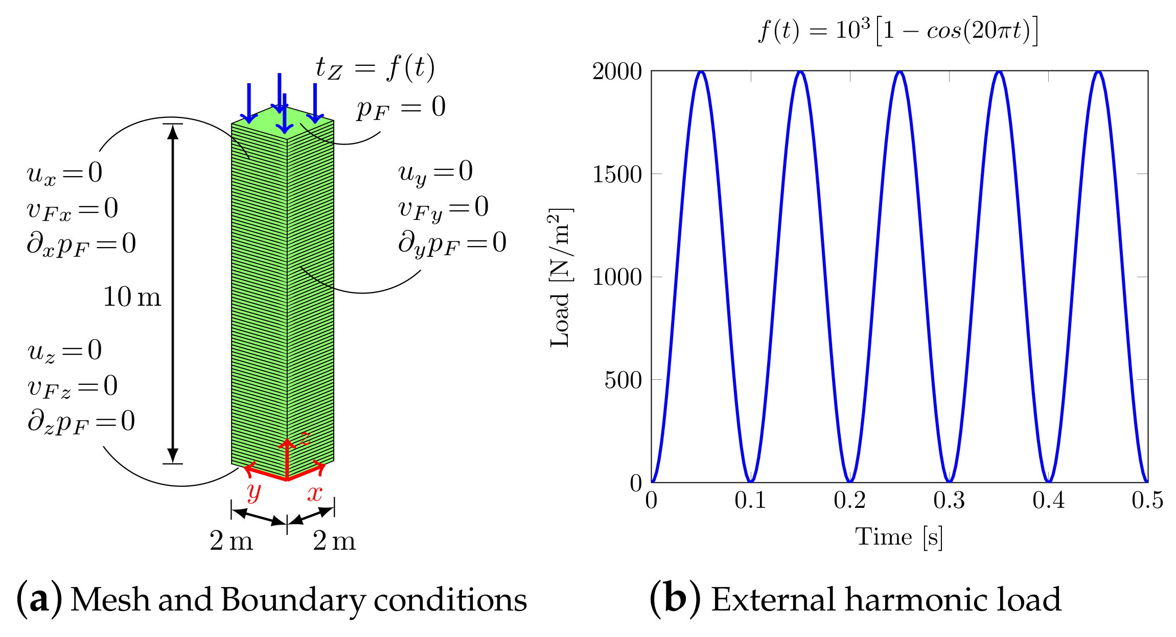
4.1. Benchmark Cases with Isotropic Elastic Materials
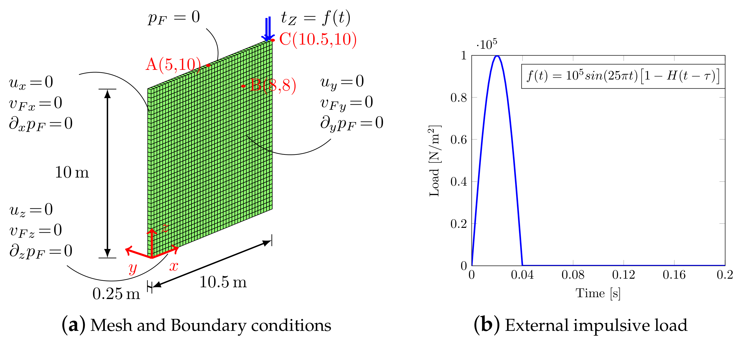
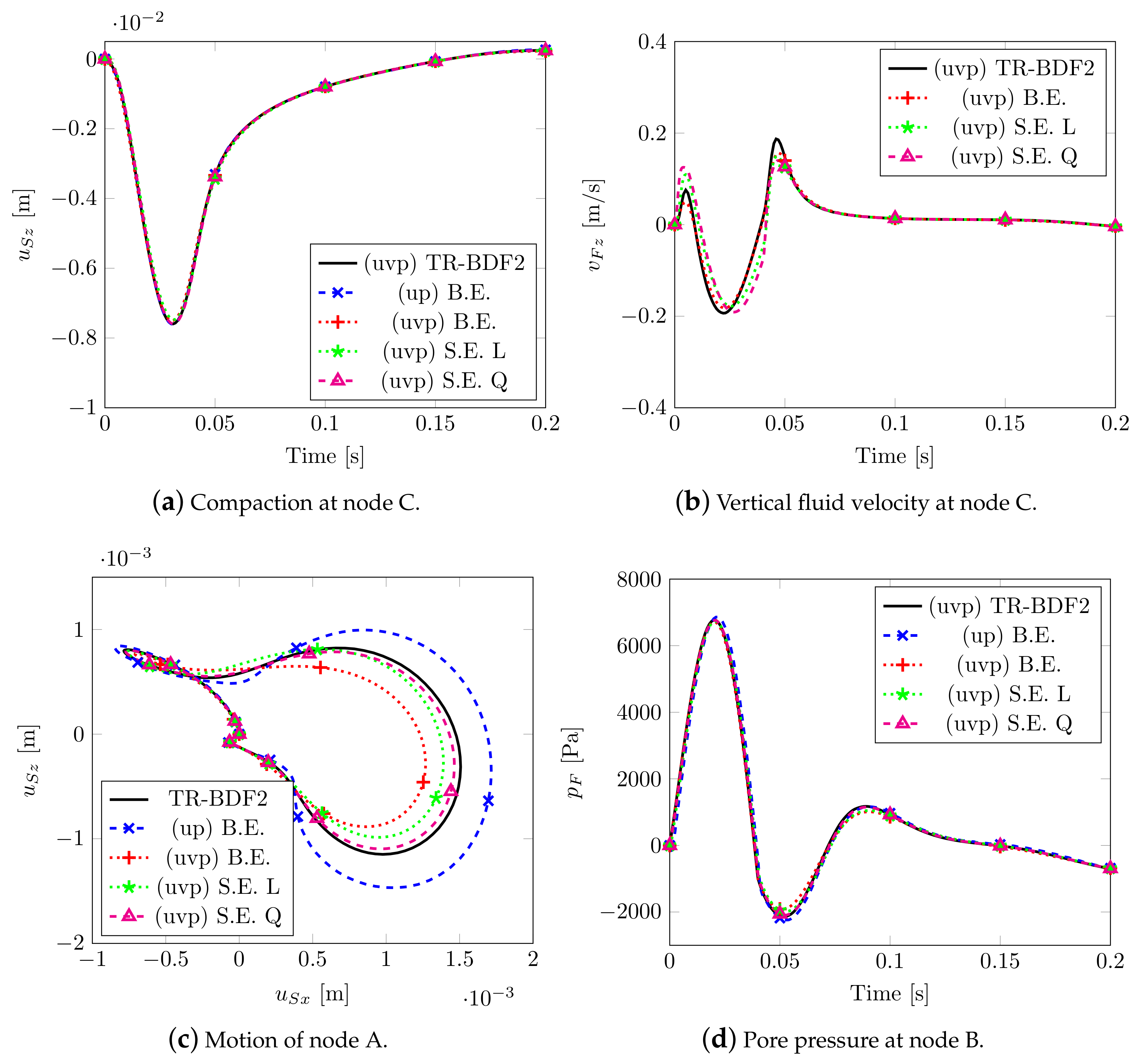
4.2. Dynamic Poroelastic Responses of Isotropic Porous Media
4.3. Dynamic Poroelastic Responses with Transversely Isotropic Porous Media
4.3.1. Effect of Different Rotation in a Transversely Isotropic Symmetry Axis of Soil Material
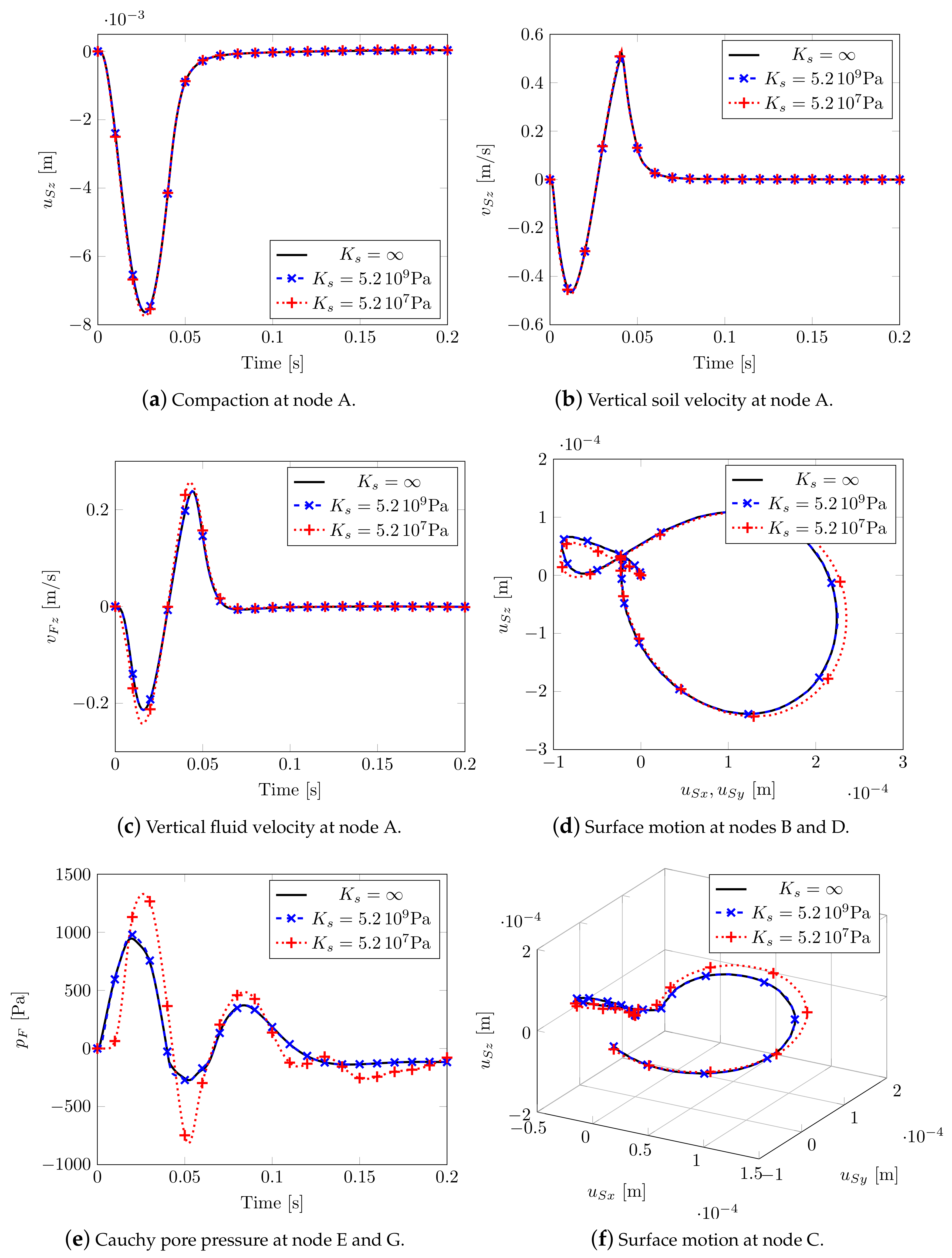
4.3.2. Effect of Biot’s Effective Stress Coefficient Tensor on Wave Propagation
5. Discussion
- (i)
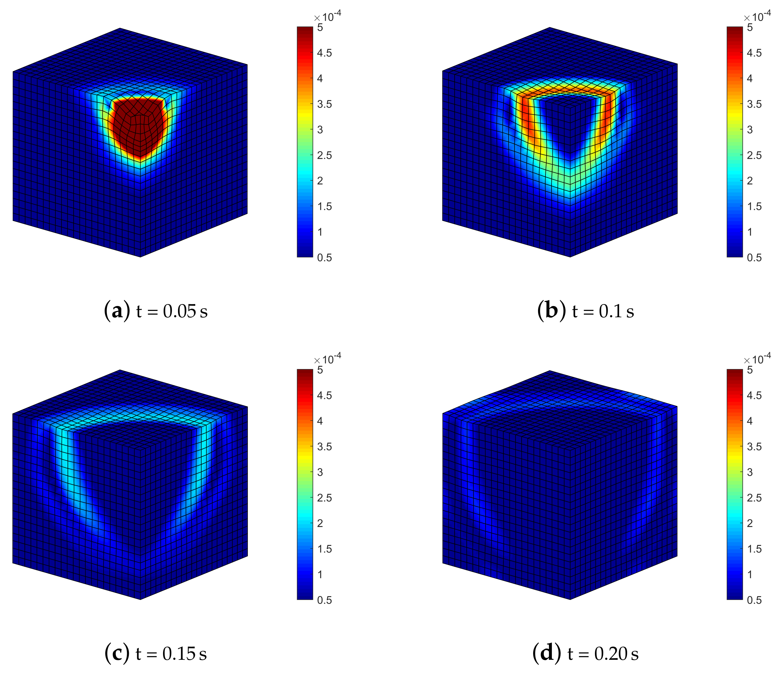
- the p-waves produce polarized vibrations along the direction of propagation (particles move along the wave’s direction of propagation) and subsequent compression and extension deformations along the same direction: they are visible along the vertical direction under the impulsive load (Figure 6 and Figure 9), even considering the anisotropic models (in this case they are coupled with the shear contribution, Figure 14 and Figure 18);
- (ii)
- p-waves are faster than s-waves: in all the models in fact the domain borders are reached in different times;
- (iii)
- (iv)
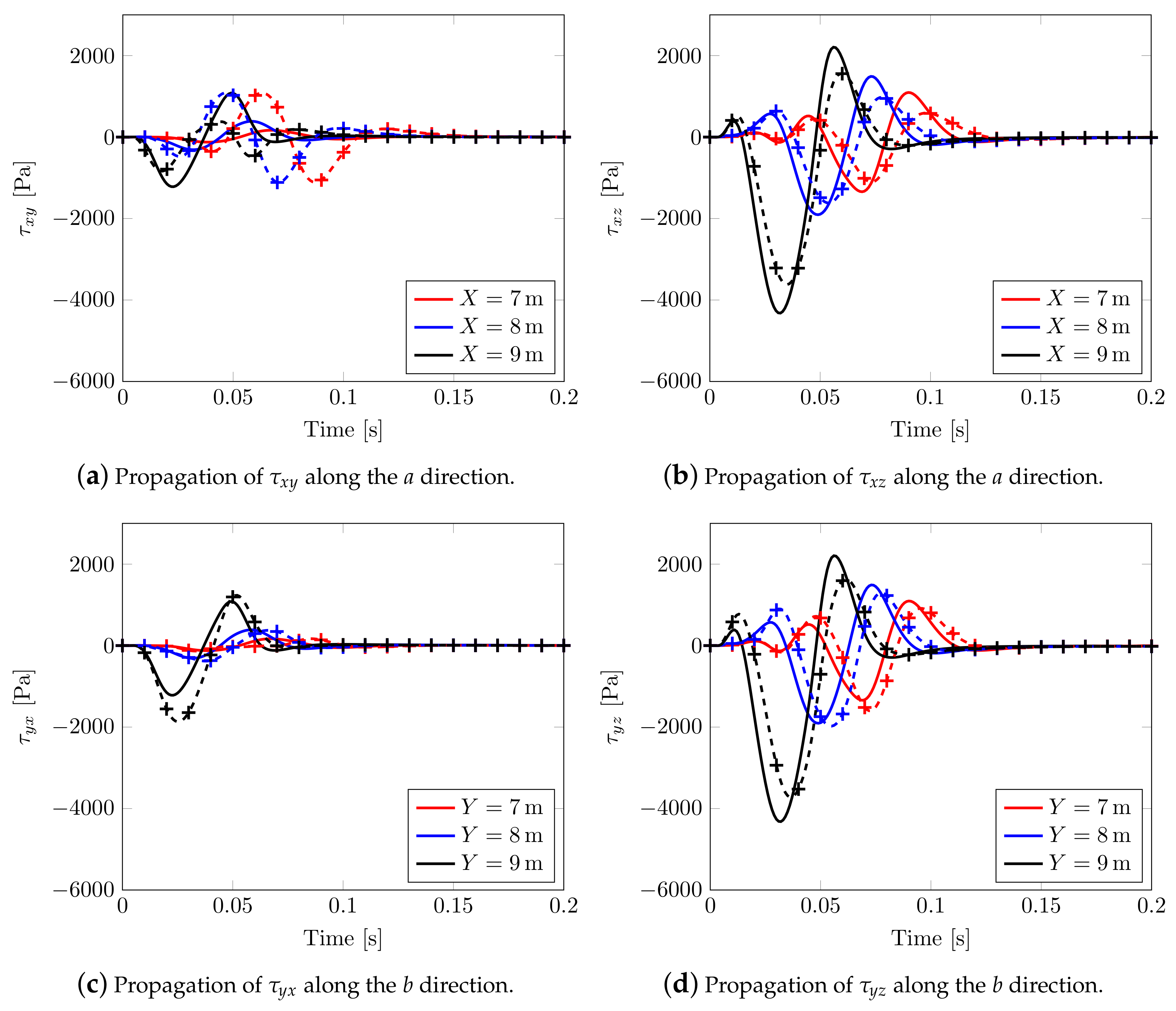
- the s-wave decouples into a wave polarized on the horizontal plane and into another one on the vertical plane: visible in the curves of effective shear stresses, Figure 15;
6. Conclusions
Author Contributions
Funding
Acknowledgments
Conflicts of Interest
Appendix A
References
- Biot, M.A. Theory of propagation of elastic waves in a fluid-saturated porous solid. II. Higher frequency range. J. Acoust. Soc. Am. 1956, 28, 179–191. [Google Scholar] [CrossRef]
- Biot, M. Theory of elastic waves in a fluid-saturated porous solid. 1. Low frequency range. J. Acoust. Soc. Am. 1956, 28, 168–178. [Google Scholar] [CrossRef]
- Berryman, J.G. Elastic wave propagation in fluid-saturated porous media. J. Acoust. Soc. Am. 1981, 69, 416–424. [Google Scholar] [CrossRef]
- Paterson, M.; Wong, T. Experimental Rock Deformation—The Brittle Field; Springer Science & Business Media: Berlin, Germany, 2005. [Google Scholar]
- Na, S.; Sun, W. Wave propagation and strain localization in a fully saturated softening porous medium under the non-isothermal conditions. Int. J. Numer. Anal. Methods Geomech. 2016, 40, 1485–1510. [Google Scholar] [CrossRef]
- Sharma, M. Propagation of seismic waves in patchy-saturated porous media: Double-porosity representation. Geophys. Prospect. 2019, 67, 2147–2160. [Google Scholar] [CrossRef]
- Borja, R.; Sun, W. Estimating inelastic sediment deformation from local site response simulations. Acta Geotech. 2007, 2, 183–195. [Google Scholar] [CrossRef][Green Version]
- Borja, R.; Sun, W. Coseismic sediment deformation during the 1989 Loma Prieta earthquake. J. Geophys. Res. Solid Earth 2008, 113, doi. [Google Scholar] [CrossRef]
- Sun, W. A unified method to predict diffuse and localized instabilities in sands. Geomech. Geoengin. 2013, 8, 65–75. [Google Scholar] [CrossRef]
- Na, S.; Sun, W.; Ingraham, M.; Yoon, H. Effects of spatial heterogeneity and material anisotropy on the fracture pattern and macroscopic effective toughness of Mancos Shale in Brazilian tests. J. Geophys. Res. Solid Earth 2017, 122, 6202–6230. [Google Scholar] [CrossRef]
- Thamarux, P.; Matsuoka, M.; Poovarodom, N.; Iwahashi, J. VS30 Seismic Microzoning Based on a Geomorphology Map: Experimental Case Study of Chiang Mai, Chiang Rai, and Lamphun, Thailand. ISPRS Int. J. Geo-Inf. 2019, 8, 309. [Google Scholar] [CrossRef]
- Crampin, S. Evaluation of anisotropy by shear-wave splitting. Geophysics 1985, 50, 142–152. [Google Scholar] [CrossRef]
- Cardoso, L.; Cowin, S.C. Role of structural anisotropy of biological tissues in poroelastic wave propagation. Mech. Mater. 2012, 44, 174–188. [Google Scholar] [CrossRef]
- Aki, K.; Richards, P.G. Quantitative Seismology, 2nd ed.; University Science Books: Mill Valley, CA, USA, 2002. [Google Scholar]
- Vlastos, S.; Liu, E.; Main, I.; Schoenberg, M.; Narteau, C.; Li, X.; Maillot, B. Dual simulations of fluid flow and seismic wave propagation in a fractured network: Effects of pore pressure on seismic signature. Geophys. J. Int. 2006, 166, 825–838. [Google Scholar] [CrossRef]
- Boxberg, M.S.; Prévost, J.H.; Tromp, J. Wave propagation in porous media saturated with two fluids. Transp. Porous Media 2015, 107, 49–63. [Google Scholar] [CrossRef]
- Crampin, S.; Peacock, S. A review of shear-wave splitting in the compliant crack-critical anisotropic Earth. Wave Motion 2005, 41, 59–77. [Google Scholar] [CrossRef]
- Grechka, V.; Kachanov, M. Effective elasticity of fractured rocks: A snapshot of the work in progress. Geophysics 2006, 71, W45–W58. [Google Scholar] [CrossRef]
- Grechka, V.; Vasconcelos, I.; Kachanov, M. The influence of crack shape on the effective elasticity of fractured rocks. Geophysics 2006, 71, D153–D160. [Google Scholar] [CrossRef]
- Crampin, S.; McGonigle, R. The variation of delays in stress-induced anisotropic polarization anomalies. Geophys. J. Int. 1981, 64, 115–131. [Google Scholar] [CrossRef]
- Virieux, J. P-SV wave propagation in heterogeneous media: Velocity-stress finite-difference method. Geophysics 1986, 51, 889–901. [Google Scholar] [CrossRef]
- Carcione, J.M. A generalization of the Fourier pseudospectral method. Geophysics 2010, 75, A53–A56. [Google Scholar] [CrossRef]
- Prevost, J.H. Wave propagation in fluid-saturated porous media: An efficient finite element procedure. Int. J. Soil Dyn. Earthq. Eng. 1985, 4, 183–202. [Google Scholar] [CrossRef]
- Sluys, L.; de Borst, R.; Mühlhaus, H. Wave propagation, localization and dispersion in a gradient-dependent medium. Int. J. Solids Struct. 1993, 30, 1153–1171. [Google Scholar] [CrossRef]
- Abellan, M.; De Borst, R. Wave propagation and localisation in a softening two-phase medium. Comput. Methods Appl. Mech. Eng. 2006, 195, 5011–5019. [Google Scholar] [CrossRef]
- Cowin, S.C.; Doty, S.B. Tissue Mechanics; Springer Science & Business Media: Berlin, Germany, 2007. [Google Scholar]
- Ehlers, W. Porous Media: Theory, Experiments and Numerical Applications; Springer Science & Business Media: Berlin, Germany, 2002. [Google Scholar]
- De Marchi, N.; Salomoni, V.; Spiezia, N. Effects of Finite Strains in Fully Coupled 3D Geomechanical Simulations. Int. J. Geomech. 2019, 19, 04019008. [Google Scholar] [CrossRef]
- White, J.; Borja, R. Stabilized low-order finite elements for coupled solid-deformation/fluid-diffusion and their application to fault zone transients. Comput. Methods Appl. Mech. Eng. 2008, 197, 4353–4366. [Google Scholar] [CrossRef]
- Sun, W.; Ostien, J.; Salinger, A. A stabilized assumed deformation gradient finite element formulation for strongly coupled poromechanical simulations at finite strain. Int. J. Numer. Anal. Methods Geomech. 2013, 37, 2755–2788. [Google Scholar] [CrossRef]
- Sun, W. A stabilized finite element formulation for monolithic thermo-hydro-mechanical simulations at finite strain. Int. J. Numer. Methods Eng. 2015, 103, 798–839. [Google Scholar] [CrossRef]
- Wang, K.; Sun, W. A semi-implicit discrete-continuum coupling method for porous media based on the effective stress principle at finite strain. Comput. Methods Appl. Mech. Eng. 2016, 304, 546–583. [Google Scholar] [CrossRef]
- Wang, K.; Sun, W. A unified variational eigen-erosion framework for interacting brittle fractures and compaction bands in fluid-infiltrating porous media. Comput. Methods Appl. Mech. Eng. 2017, 318, 1–32. [Google Scholar] [CrossRef]
- Na, S.; Bryant, E.C.; Sun, W. A configurational force for adaptive re-meshing of gradient-enhanced poromechanics problems with history-dependent variables. Comput. Methods Appl. Mech. Eng. 2019, 357, 112572. [Google Scholar] [CrossRef]
- Carroll, M. An effective stress law for anisotropic elastic deformation. J. Geophys. Res. Solid Earth 1979, 84, 7510–7512. [Google Scholar] [CrossRef]
- Nur, A.; Byerlee, J. An exact effective stress law for elastic deformation of rock with fluids. J. Geophys. Res. 1971, 76, 6414–6419. [Google Scholar] [CrossRef]
- Sun, W.; Andrade, J.; Rudnicki, J.; Eichhubl, P. Connecting microstructural attributes and permeability from 3D tomographic images of in situ shear-enhanced compaction bands using multiscale computations. Geophys. Res. Lett. 2011, 38. [Google Scholar] [CrossRef]
- Cowin, S.C. Continuum Mechanics of Anisotropic Materials; Springer Science & Business Media: Berlin, Germany, 2013. [Google Scholar]
- Markert, B.; Heider, Y.; Ehlers, W. Comparison of monolithic and splitting solution schemes for dynamic porous media problems. Int. J. Numer. Methods Eng. 2010, 82, 1341–1383. [Google Scholar] [CrossRef]
- Jansen, K.E.; Whiting, C.H.; Hulbert, G.M. A generalized-α method for integrating the filtered Navier–Stokes equations with a stabilized finite element method. Comput. Methods Appl. Mech. Eng. 2000, 190, 305–319. [Google Scholar] [CrossRef]
- Huang, M.; Wu, S.; Zienkiewicz, O. Incompressible or nearly incompressible soil dynamic behaviour—A new staggered algorithm to circumvent restrictions of mixed formulation. Soil Dyn. Earthq. Eng. 2001, 21, 169–179. [Google Scholar]
- Huang, M.; Yue, Z.Q.; Tham, L.; Zienkiewicz, O. On the stable finite element procedures for dynamic problems of saturated porous media. Int. J. Numer. Methods Eng. 2004, 61, 1421–1450. [Google Scholar]
- De Boer, R.; Ehlers, W.; Liu, Z. One-dimensional transient wave propagation in fluid-saturated incompressible porous media. Arch. Appl. Mech. 1993, 63, 59–72. [Google Scholar] [CrossRef]
- Yang, Z.; Li, Z. A numerical study on waves induced by wheel-rail contact. Int. J. Mech. Sci. 2019, 161, 105069. [Google Scholar] [CrossRef]


| Parameter | Values | S.I. unit |
|---|---|---|
| E | 14.52 × 10 | Pa |
| 0.30 | ||
| 0.33 | ||
| 10 | m/s | |
| 2000 | kg/m | |
| 1000 | kg/m |
| Parameter | Values | S.I. Unit |
|---|---|---|
| E | 12.0 × 10 | Pa |
| 0.25 | ||
| 0.33 | ||
| 10.0 | m/s | |
| 2000.0 | kg/m | |
| 1000.0 | kg/m | |
| 5.2 × 10 | Pa |
| Parameter | Values | S.I. Unit |
|---|---|---|
| 9 × 10 | Pa | |
| 15 × 10 | Pa | |
| 0.25 | ||
| 0.21 | ||
| 0.35 | ||
| 3.6 × 10 | Pa | |
| 6.0 × 10 | Pa | |
| 0.33 | ||
| 10 | m/s | |
| 10 | m/s | |
| 2000 | kg/m | |
| 1000 | kg/m | |
| 7.14 × 10 | Pa | |
| 3.57 × 10 | Pa | |
| 2.2 × 10 | Pa |
| Parameter | Values | S.I. Unit |
|---|---|---|
| 1.8 × 10 | Pa | |
| 3.0 × 10 | Pa | |
| 0.25 | ||
| 0.21 | ||
| 0.35 | ||
| 7.2 × 10 | Pa | |
| 1.2 × 10 | Pa |
Publisher’s Note: MDPI stays neutral with regard to jurisdictional claims in published maps and institutional affiliations. |
© 2020 by the authors. Licensee MDPI, Basel, Switzerland. This article is an open access article distributed under the terms and conditions of the Creative Commons Attribution (CC BY) license (http://creativecommons.org/licenses/by/4.0/).
Share and Cite
De Marchi, N.; Sun, W.; Salomoni, V. Shear Wave Splitting and Polarization in Anisotropic Fluid-Infiltrating Porous Media: A Numerical Study. Materials 2020, 13, 4988. https://doi.org/10.3390/ma13214988
De Marchi N, Sun W, Salomoni V. Shear Wave Splitting and Polarization in Anisotropic Fluid-Infiltrating Porous Media: A Numerical Study. Materials. 2020; 13(21):4988. https://doi.org/10.3390/ma13214988
Chicago/Turabian StyleDe Marchi, Nico, WaiChing Sun, and Valentina Salomoni. 2020. "Shear Wave Splitting and Polarization in Anisotropic Fluid-Infiltrating Porous Media: A Numerical Study" Materials 13, no. 21: 4988. https://doi.org/10.3390/ma13214988
APA StyleDe Marchi, N., Sun, W., & Salomoni, V. (2020). Shear Wave Splitting and Polarization in Anisotropic Fluid-Infiltrating Porous Media: A Numerical Study. Materials, 13(21), 4988. https://doi.org/10.3390/ma13214988