3.1. The Analytical Approach
The identification of mode shapes significantly improves the results of the optimization of stacking sequence in composite structures (see [
6,
11]); therefore, it is analyzed in detail in this paper.
The initial FE model is biaxially symmetric. The mode shapes of natural vibrations can be divided into Axial (A0m, ), Torsional (T0m, ), Bending (B1m, ), and Circumferential ones (C, , ).
The mode shape code, X, shows that the mode shape family (X is replaced by A for axial, T for torsional, B for bending, and C for circumferential mode shape), circumferential wave w, and axial mode x. As a rule, different mode shapes correspond to unique natural frequencies; for axisymmetric FE models, close values of the natural frequencies of adjacent vibration modes can be observed (e.g., ).
Mode shapes identification and assigning them to appropriate classes simplifies the analysis and allows building simple and effective tools for the optimization and diagnosis of the structure under study [
6,
11]. For the initial model (see
Figure 2), with no defects and/or material degradation, it is possible to create an analytical procedure for the identification of mode shapes (see [
11]). The procedure in the form described in [
11] relies on the analysis of the movement of the FE model node with the highest displacement magnitude. This approach, which is fast and effective for biaxially symmetric structure, is not reliable enough for the structure with local material degradation and/or geometric uncertainties, which in turn leads to the loss of symmetry (especially for large areas of material degradation). In what follows an automatic, neural network-based, identification of mode shapes is presented. However, the analytical method is still applied in the new approach; the learning and testing patterns were built using the results of the identification performed by the analytical procedure.
3.2. Neural Network Based Mode Shapes Identification
The range of the analyzed natural frequencies was limited here with the value 100 Hz, which seems to be a reasonable restriction from the point of view of the civil engineering analysis. The mode shapes corresponding to the natural frequencies lower than 100 Hz are the following ones: A01 (one axial mode), B11 and B12 (two bending modes), C21, C22, C23, C31, C32, C33, C41 and C42 (eight circumferential modes), and T01 (one torsional mode). The majority of them are—for biaxially symmetric structures—double mode shapes (i.e., two corresponding natural frequencies are almost equal and the corresponding mode shapes differ only in rotation about the structure axis of symmetry), and the overall number of the analyzed frequencies thus reaches 22 (10 of 12 considered modes are double ones).
To identify the above-listed mode, CNNs are applied. Although CNNs are particularly suited to image analysis, they can also efficiently analyze numerical sets. The training of CNN is performed using a set of examples (called patterns); here, each of the examples (patterns) consists of a 240-element input matrix (
) describing the analyzed mode shape (three mode shape components—displacements along three Cartesian coordinate system axes—in 20 nodes of four cross-sections of the FE model (see
Figure 4)), and one-element desired output showing the mode shape name (obtained from the analytical identification procedure). The CNN output may be presented using either the usual classification approach (the name of the identified mode shape) or a vector, where each of the vector elements shows the level of similarity to one of the considered mode shapes. The output vector contains the values from the range
, and the identified mode shape is chosen as the one corresponding to the maximal element of the output vector.
To reduce the dimensions of the input matrix, the description of each mode shape is reduced, as mentioned above, to
matrix. The selected 20 nodes in each of the selected four cross-sections are chosen as every fourth node in each of the cross-sections A, B, C, and D in
Figure 4; the cross-sections are located 6.0 m, 4.5 m, 3.0 m or 1.5 m away from the fixed end of the cylinder.
To verify the accuracy of the proposed identification method, four different numbers of layers of composite material were considered: . For each value of n (with the shell thickness constant for all the considered cases), 2000 random lamination angles sets were generated, and in each case, 12 mode shapes were considered (as described above: one axial mode, two bending modes, eight circumferential modes, and one torsional mode). Only axial and torsional modes are single modes; however, in the case of double modes, the corresponding mode shapes are not identical; they are rotated around the axis of the cylinder. The inclusion of both double mode shapes increases the accuracy of the procedure. The overall number of considered modes reached 24 () for each of the models since axial and torsional modes (single ones) were also repeated. Altogether, 192,000 patterns were obtained (one model generated 24 patterns; the number of models was equal to 2000 for each number of n).
The patterns were divided into learning and testing sets: all the cases generated for
and
composite layers were used as learning patterns while the cases with
and
layers were used at the testing stage. The number of learning patterns was the same as the number of testing patterns—in both cases, 96,000. However, the analytical identification procedure—used as the reference procedure—failed to identify A01 mode shape in some of the considered cases, and the number of corresponding patterns was slightly smaller (see
Figure 5).
The results of learning and testing of CNN network (called in what follows CNN-
) are shown in
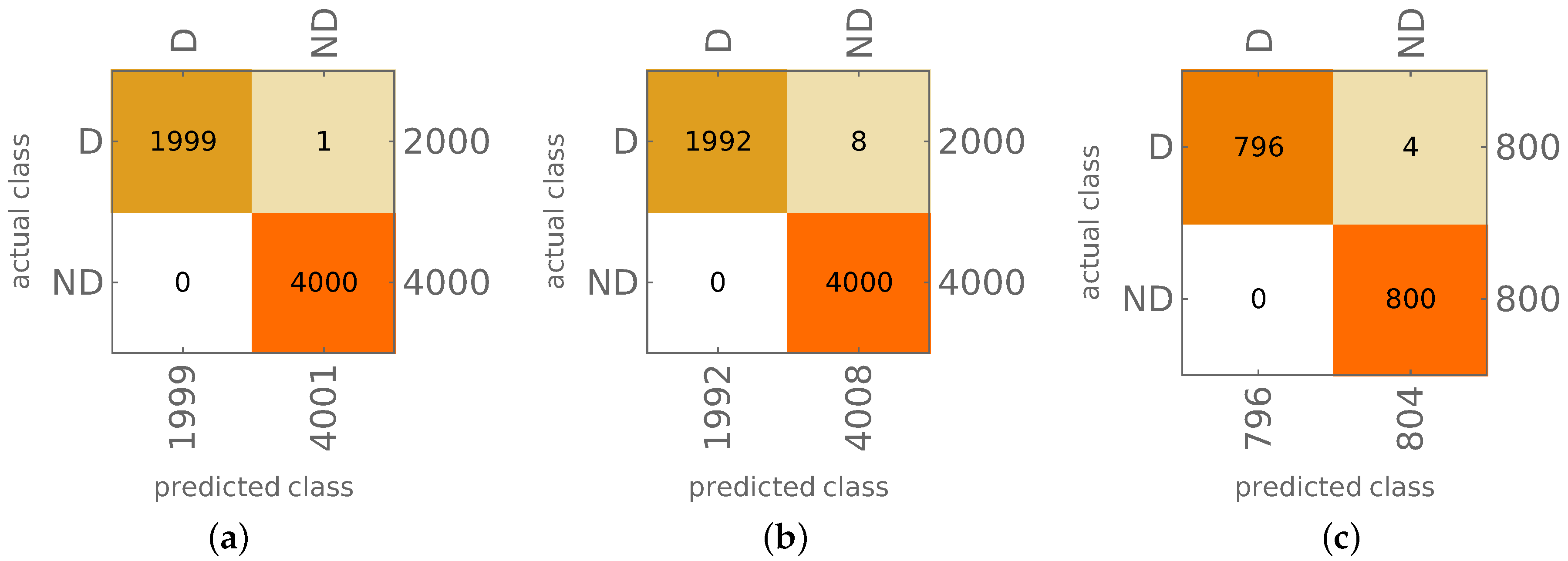
Figure 5. The figure shows the confusion matrix, where the vertical axis presents the target mode shape (identified using the analytical reference procedure) and the horizontal axis shows the CNN-identified (predicted) mode shape. The numbers on the right-hand side or below the plot show the overall number of cases in a particular row (the proper number of cases representing a particular mode shape) or column (the number of cases predicted as a particular mode shape).
In case of faultless identification of all mode shapes, there should be no cases outside the diagonal of the confusion matrix and the number of cases in the corresponding row and column should be equal. There are a few errors in the results shown in
Figure 5; however, their number is negligible. The level of accuracy of the identification of testing mode shapes reaches almost 100%.
It has to be noted that in some selected cases, a result classified as incorrect in comparison with the reference analytical procedure may be in fact correct, because the analytical procedure also may incorrectly identify the mode shape in question. However, such cases are few and do not affect the accuracy of the CNN procedure.
The trained CNN-
was also verified using mode shapes obtained from the same FE model with some material constants altered; the values of Young’s moduli were changed to
GPa and
GPa (while the original moduli were
GPa,
GPa). The results of mode shapes identification are shown in
Figure 6; the number of models with altered material constants equals 800 (200 different lamination angles cases for each
n). The results shown in
Figure 6 prove that the CNN trained on a model with constant shell thickness and material properties is able to properly predict mode shapes for a structure made of a different material.
Further verification of the robustness of the proposed mode shapes identification procedure involves artificial, random disturbing of mode shapes obtained from numerical simulations. Random noise can emulate some measurements errors, inevitable during real experiments. The mode shapes obtained from numerical simulations were processed in three consecutive steps:
each of the four cross-sections was shifted by a random vector (the same for the whole cross-section),
each node on each of the four cross-sections was shifted by a random vector (unique for each node),
the accuracy of each mode shape element was truncated to l significant digits.
In each case, the considered random noise was of a Gaussian distribution. The above described three steps can be described using simple formulas. The random shift of each mode shape cross-section is governed by the Equation:
where
is the original location of the considered cross-section (i.e.,
contains in-plane coordinates of each of the 20 points of a particular cross-section), and
is a random shift vector (its coordinated are generated using Gaussian distribution with mean equal to 0 and
standard deviation),
where
are the randomly shifted (see Equation (
5)) coordinates of each of mode shape nodes and
is the random coordinate multiplayer, unique for each mode-shape node (Gaussian distribution with mean equal to 1 and
standard deviation),
where
is an operator of truncation to
l significant digits.
The network trained and tested on noisy data is called in what follows CNN-
. Different values of
,
and
l were considered; for each of them, the proposed identification method is robust and guarantees a high identification accuracy.
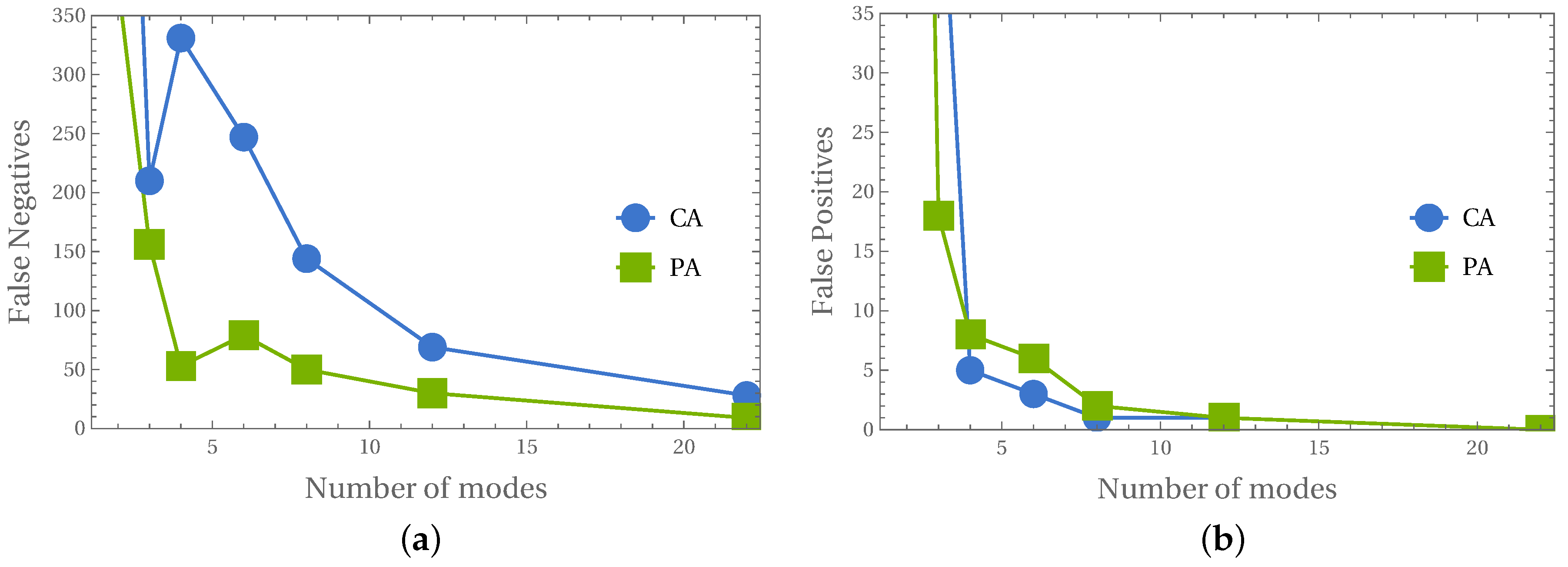
Figure 7 shows the identification results obtained for
and
. The value of
l, while it is not lower than 4, has negligible influence on the results.
In
Table 2, we present the number of wrong identification cases obtained during learning and testing for all of the above-described cases. As can be seen, the percentage of errors is small (the values in the parenthesis show the overall number of mode shapes being identified in a particular case).
It should be noted that the analytical reference procedure properly identifies the mode shape family (axial, bending, circumferential, and torsional) only for noised mode shapes with standard deviations not higher than and ( ten times smaller than the smallest one considered for CNN identification procedure), but the circumferential waves are already misidentified. For and (the smallest level of noise considered for CNN identification), the analytical identification is wrong in all cases considered, including the misidentification of the mode shape family. Although the analytical procedure can be improved and better results can certainly be obtained, the experience gained by the authors shows that the results will not be comparable to the CNN results. The analytical procedure is not robust to a larger error, even in just one coordinate among the considered three.
In addition to CNNs, the usefulness of deep learning feedforward neural networks (FFNNs) was also verified. The results are gathered in
Table 3, and although the mode shapes identification is rather precise, the advantage of CNNs over FFNNs is clearly visible. The reason for the higher accuracy of CNNs may be related to a different processing method. Moreover, as it is shown in
Table 2 and
Table 3, the number of patterns in learning sets reaches 96,000; CNNs are well suited to analyze such multielement learning sets.
3.3. Identification of Mode Shapes Obtained from the Model with Material Degradation
To verify the ability of the proposed CNN-
network to identify mode shapes obtained from a model with some changes and damages, possibly causing mode shapes changes and/or the lack of model axial symmetry, some local changes were introduced to the model. In a randomly selected area of the model, the material constants of half of the shell layers were reduced, namely, Young’s moduli are in these layers as follows:
GPa,
GPa (instead of original values
GPa,
GPa). The area with material constants degradation consisted of
r rows and
c columns of finite elements; in all the cases,
, so the degradation area was—for simplicity—considered to be “square” (in fact, it is a section of the cylindrical shell). The location of this square area was selected at random without any limitations over the entire shell; the size was limited up to 144 elements (
, for
) so its biggest size was as high as approximately 1.5% of the whole area of the shell (see
Figure 8) while the smallest size (
elements) was as small as 0.04% of the whole area of the shell.
Accordingly, all the cases with and composite layers were used as learning patterns, whereas the cases with and layers were used at the testing stage. The number of learning patterns was the same as the number of testing patterns; in both cases, it was equal to 144,000 (96,000 patterns obtained from the models without damage and 48,000 patterns obtained from the models with material degradation). The patterns were FEM-generated for the model with random lamination angles and material degradation zone location and size following the previously described assumptions.
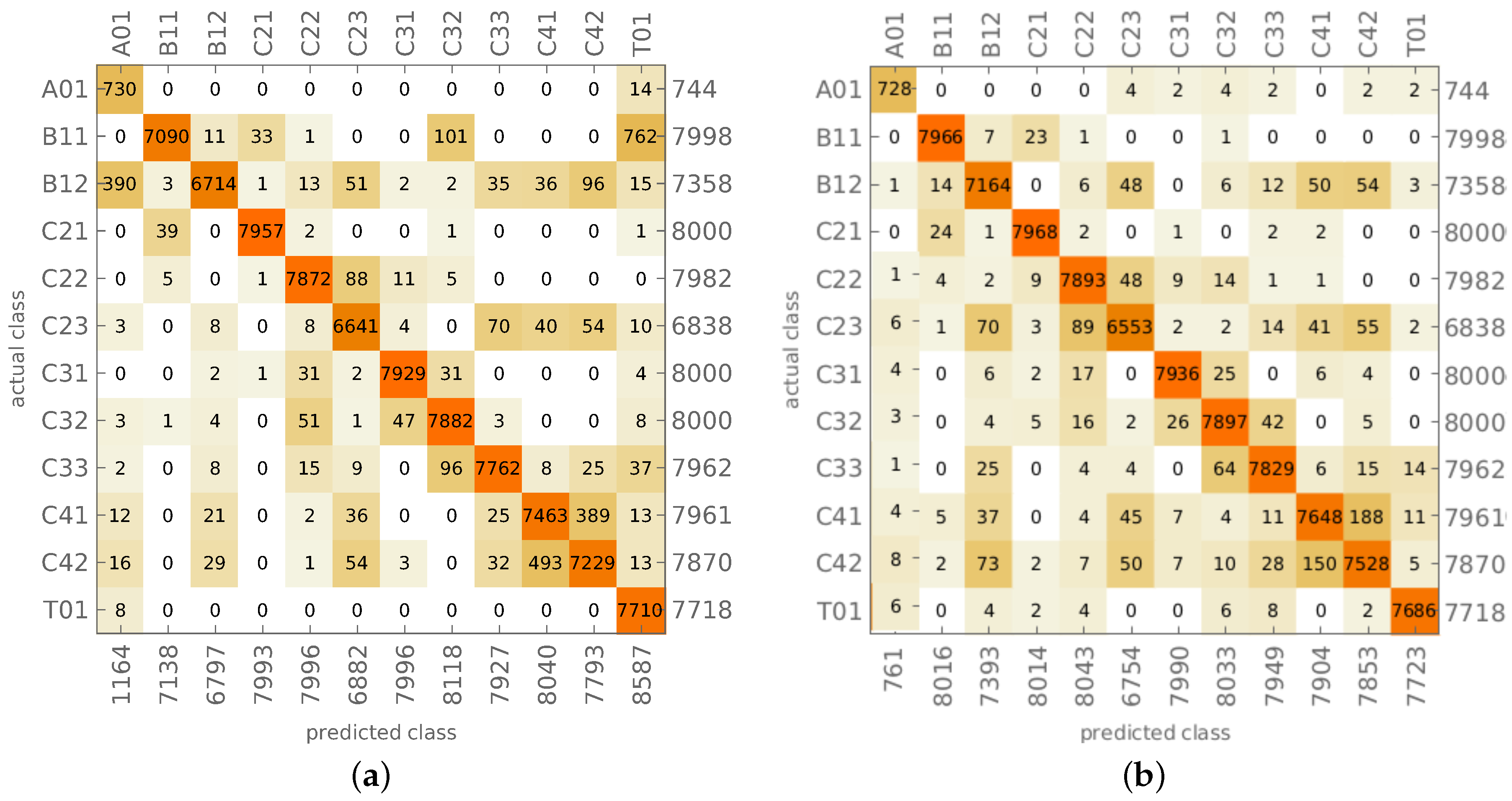
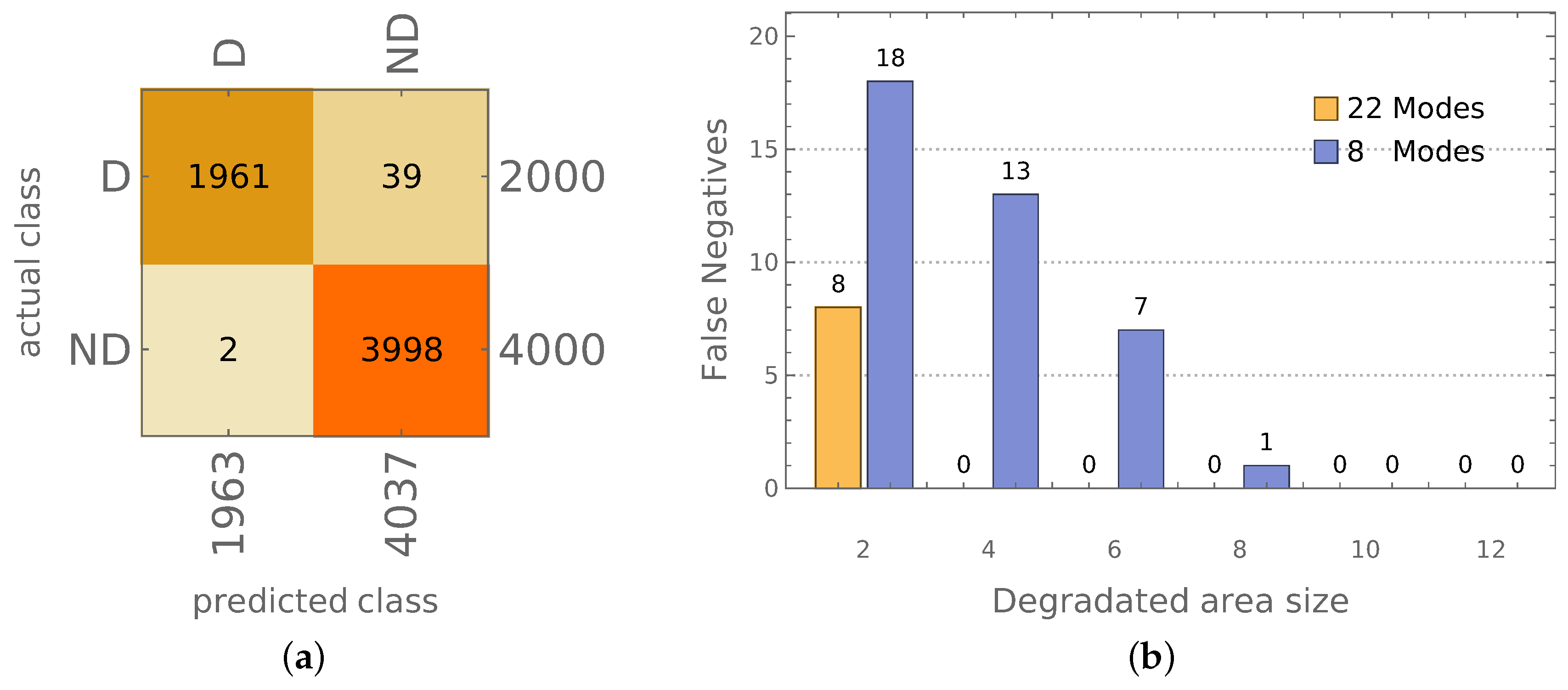
Figure 9a shows the results of mode shapes identification performed using CNN-
described in the previous subsection (learned using only data from models without material degradation). The overall accuracy of mode shapes identification is equal to 96.01%; the CNN-
network is rather precise also for the models with material degradation. The mistakes are mainly related to the identification of bending shapes (B11, B12) and circumferential shapes with fourth circumferential wave (C41, C42); the reason for these errors may be the limited number of considered cross-sections (only four). The number of examples in each of the identified classes differs from 8000 because the reference analytical procedure fails to identify some mode shapes obtained from models with material degradation.
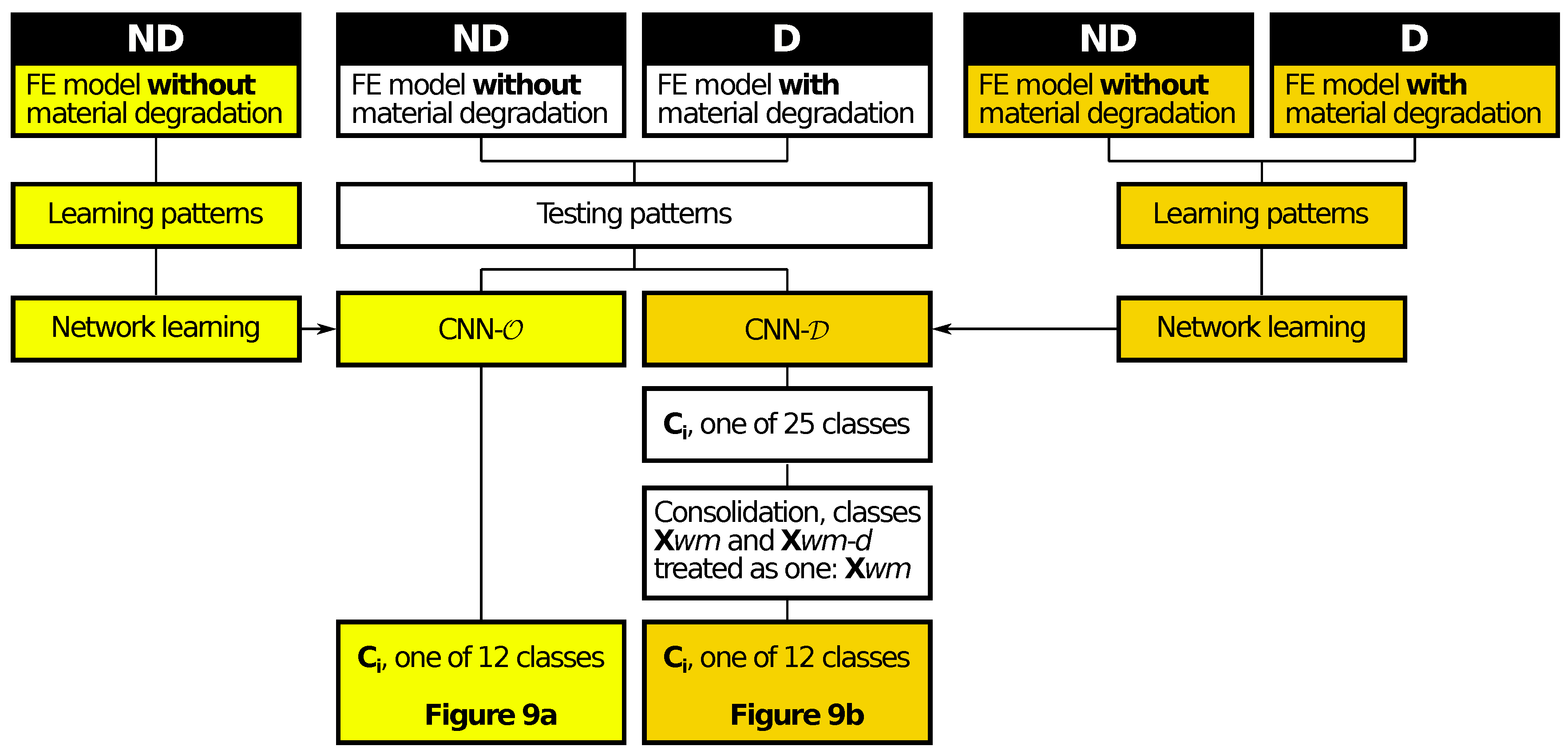
To improve the results for models with material degradation, the identification CNNs were created again using a few different approaches. The task of the CNN was to identify:
24 classes: both the mode shape and the state of the structure (with or without material degradation); the number of mode shapes classes being identified was equal to 24, the additional ones were A01d, B11d, B12d, C21d, C22d, C23d, C31d, C32d, C33d, C41d, C42d and T01d (where d stands for material degradation),
25 classes: both the mode shape and the state of the structure (with or without material degradation) with an additional 25th class for unrecognized mode shapes; the additional class corresponds to cases where the analytical procedure failed to recognize the mode shape,
25 classes (two stage CNN learning): stage I: learning on patterns without material degradation, stage II: additional learning on patterns with material degradation; such approach is suggested for this kind of networks [
41], the obtained network is called CNN-
in what follows.
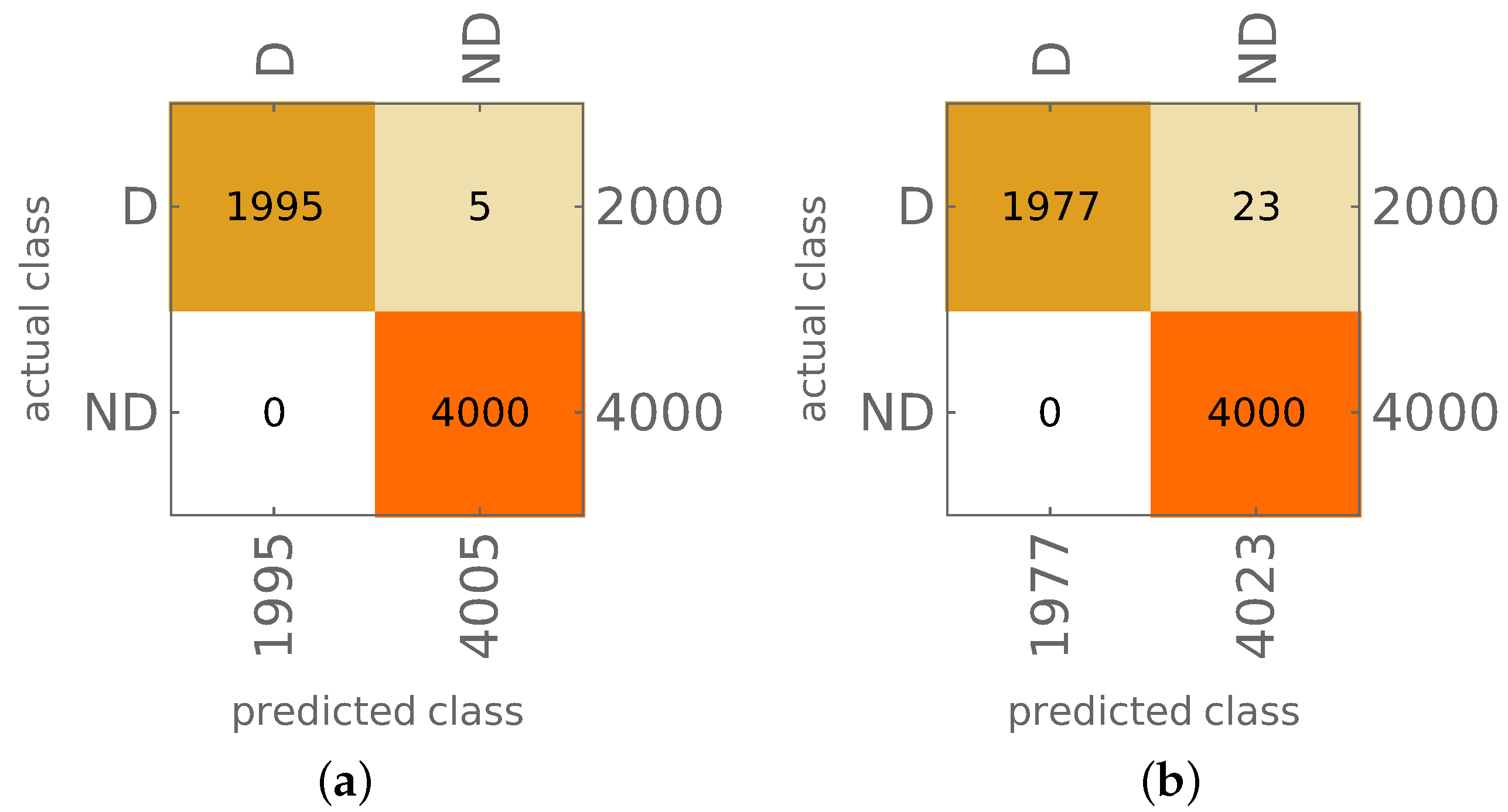
The results are gathered in
Table 4; the relative accuracy is related to 24 classes (the classes
and
d, e.g., C21 and C21
d, were treated as separate ones).
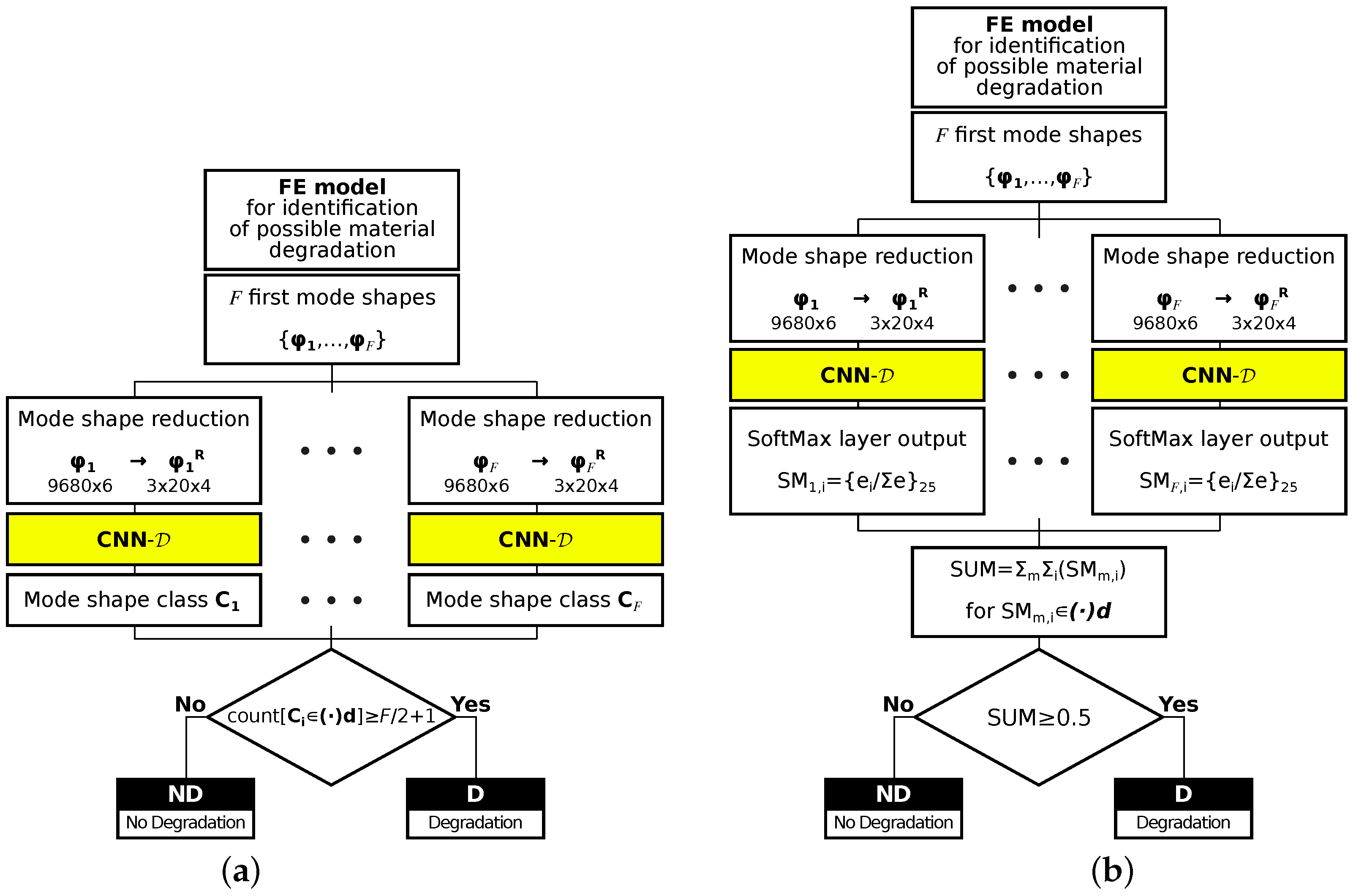
In order to compare the results with the ones presented in
Figure 9a, the results obtained from the 25-classes approach were transformed into 12 classes, where the information about material model degradation was neglected (the classes
and
d, e.g., C21 and C21
d, were treated as one), see
Figure 9b and
Figure 10 (an algorithm). The accuracy of the mode shape identification, neglecting the information concerning the model state, reaches 98.11% (this value is higher than the accuracy presented in
Table 4 since it ignores the differences between
and
d classes).


