2.1. Dynamic Equation of the Thin Plate
In the physical model, a flexible thin plate with four edges clamped conditions was adopted. The governing equation of the plate can be formulated as a partial differential equation (PDE) together with the corresponding boundary conditions and by assuming small lateral deflection conditions, one may have [
29]:
where
denotes the deflection of the mid-plane of the plate,
is the density of plate with dimension mass per unit volume,
is the transverse external force with the dimension of force per unit area,
is the flexural rigidity,
is the elastic modulus of the plate material,
is the thickness and
is the Poisson’s ratio. In the rectangular coordinate system, for
are clamped edges, then the boundary condition is as follows:
For simulation purposes, it is natural to assume that the forces and moments of the plate due to its weight are neglected. In other words, the plate has no deflection initially. Thus, for every point located on the plate, the displacement at
is assumed to be zero:
On the other hand, in the case of a plane stress problem, the constitutive equation of a homogeneous isotropic piezoelectric element can analogy for the one-dimensional problem studied by Lee and Kim [
30] and Park [
31], written as:
where
and
are the stress and strain components, respectively.
and
denote the components of the electrical field and electrical displacement, correspondingly. The superscripts (
) and (
) indicate that the material properties were measured under constant electrical and tension fields, respectively. Moreover,
is the piezoelectric constant,
interprets the dielectric constant measured under a constant tension field, and
denotes the appropriate Poisson’s ratio. Equation (4) indicates the existence of two equal in-plane strains
and
for any applied voltages along the polling axis of the piezoelectric patch. The piezoelectric patch thickness is presumably small enough to maintain a uniform and constant electric displacement over its thickness.
As shown in
Figure 1, consider bonding a piezoelectric patch on the upper surface of a thin rectangular plate with the
Z-axis pointing upward. It is assumed that the piezoelectric patch layer covers the plate from locations
to
in the
direction and from
to
in the
direction. The dimensions of the piezo patch along the
and
axes are specified by
and
, respectively. The kinetic energy of the plate and the piezo patch are the following:
where:
and:
In the above equations,
represents the mass per unit area,
represents the area of the plate, and
represents the derivatives concerning time. Also:
where
is the Heaviside step function. On the other hand, assuming that the strain is extremely small, the strain energy of the plate and the piezoelectric patch becomes:
where:
and:
The parameter
is the bending stiffness of the piezoelectric patch,
is the thickness of the piezo patch and
. Finally, applying Hamilton’s principle:
Thus, the following constitutive equations of system motion and related natural and geometric boundary conditions are derived [
32]:
where the term
is a differential operator equivalent to
, and
stands for finding the partial derivative of
first and then finding the partial derivative of
twice.
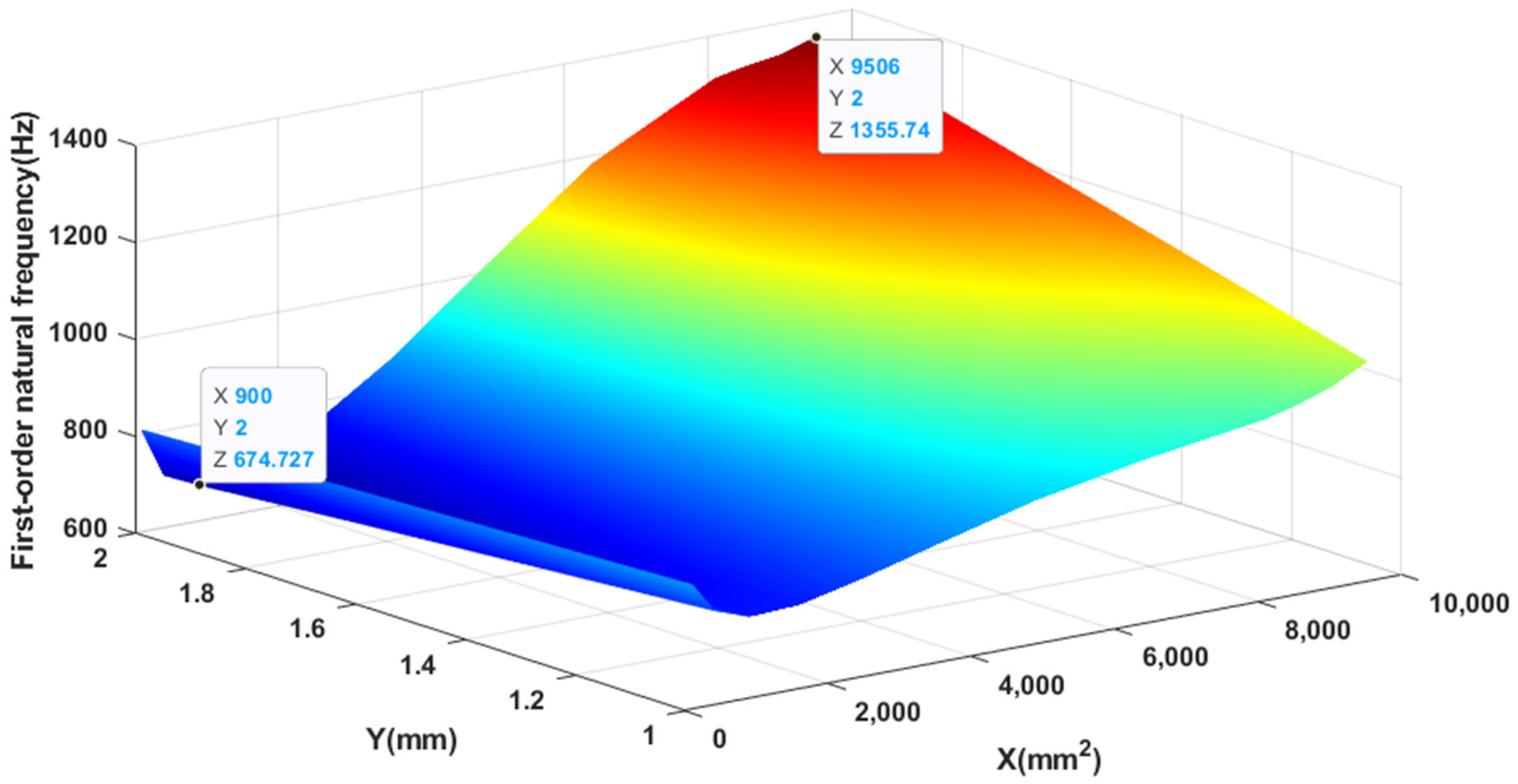
To solve Equation (13), one needs to assume that the thickness ratio of the piezoelectric plate is small so that the position of the neutral plane of the main plate can be kept unchanged with acceptable accuracy in the presence of the piezoelectric patch. Besides, since in most practical situations, the elastic modulus of piezoelectric materials is smaller than that of the motherboard, the position of the neutral plane of the combined system relative to the motherboard changes even less. In the open literature, the effect of piezoelectric patch dimension on the dynamic responses was usually ignored so that Equation (13) can be simplified to a pure elastic plate model. However, when the piezoelectric patch size is comparable to the plate, the dimension of the piezoelectric patch can significantly influence the natural frequency and displacement amplitude of the structure, which may cause inaccuracy to vibration and sounds radiation control. In the next parts, an ANN model will be built with the help of finite element simulation to explore the dimension effect of the piezoelectric patch on the structural dynamic responses.
2.2. Neural Network Modeling
The main advantage of ANN is that it can model a problem using examples rather than analytical descriptions. To study the dynamic behavior of the rectangular thin plate system considering the piezoelectric patch size effect, a computer program was written to conduct in-depth research with the help of the neural network toolbox. The complete algorithm structure of a conventional ANN includes at least three different layers: the input layer, hidden layer, and output layer. Each neuron inter-connects with all the neurons in the following layer. With a proper activation function, a combination of optimized weights can generate the prediction of the dependent variable:
where
represents the weight value of a connection,
represents an inputted independent variable, and
represents a deviation. For the activation function, the logsig function in Equation (15) is the sigmoid function in logistic regression. The input value of the Log-sigmoid function can take any value, and the output value is between 0 and 1. The input and output values of the linear transfer function purelin can take any value:
An ANN model needs to be trained from an existing training set including many pairs of input-output elements., until the root mean square error (
RMSE) between the training output data and the predicted output are minimized, as given in Equation (16):
where
represents the predicted value outputted by the ANN,
is the actual value, and
represents the total number of samples.
In this study, a typical multilayer neural network with one hidden layer is used, the network has two inputs and two output values. The proposed ANN model shown in
Figure 2 was trained by the input data obtained from COMSOL. The input layer needs many sets of data including the side length of the plate and the thickness of the piezoelectric patch. Also, the output layer gives the predicted natural frequency and displacement amplitude. The neurons in hidden layers all use a sigmoid transfer function and the neurons in the output layer use a linear transfer function. Trainbr (Bayesian regularization algorithm) modified the Levenberg-Marquardt algorithm to improve the generalization ability of the network. At the same time, the difficulty of determining the optimal network structure is reduced. The interconnection between processing units in a neural network is distributed through weights. These weights can be adjusted through the training process to optimize the neural network output.


