
Analysis of the Compression Behaviour of Reinforced Photocurable Materials Used in Additive Manufacturing Processes Based on a Mask Image Projection System

 , and
, and
Abstract
:1. Introduction
2. Materials and Methods
2.1. Formulation of Reinforced Photocurable Materials
2.2. Analytical Model Based on a Frontal Photopolymerization Process
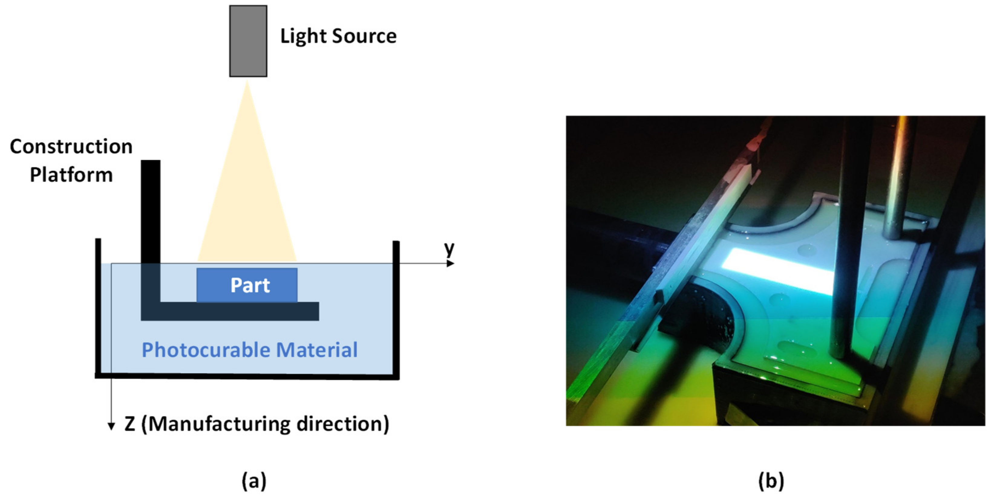
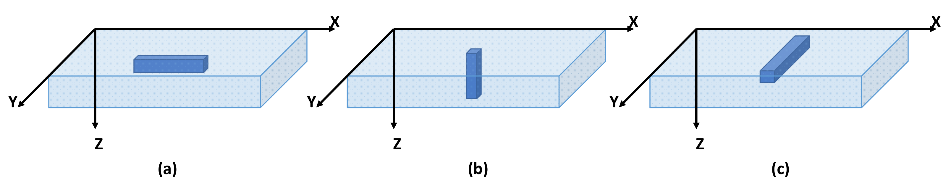
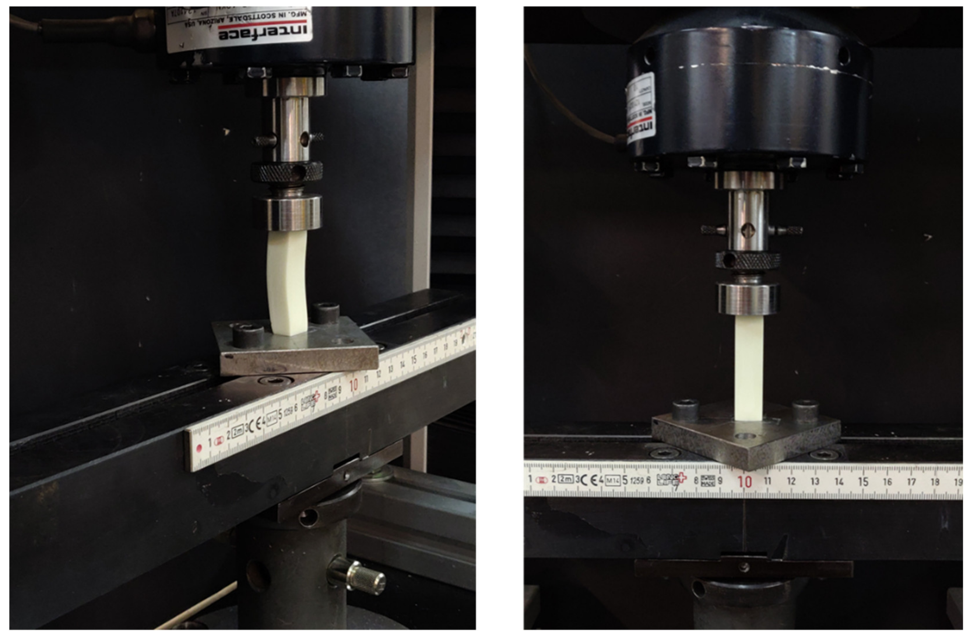
2.3. Specimens and Experimental Setup for Compression Tests
3. Results and Discussion
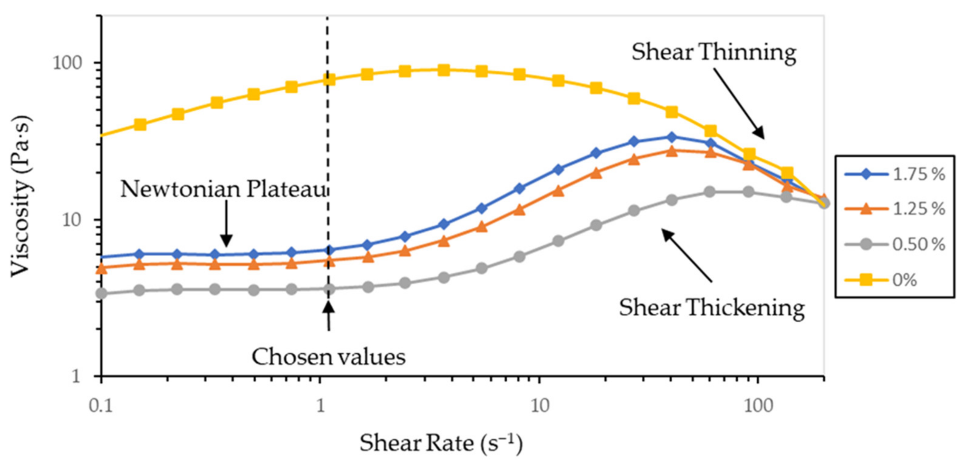
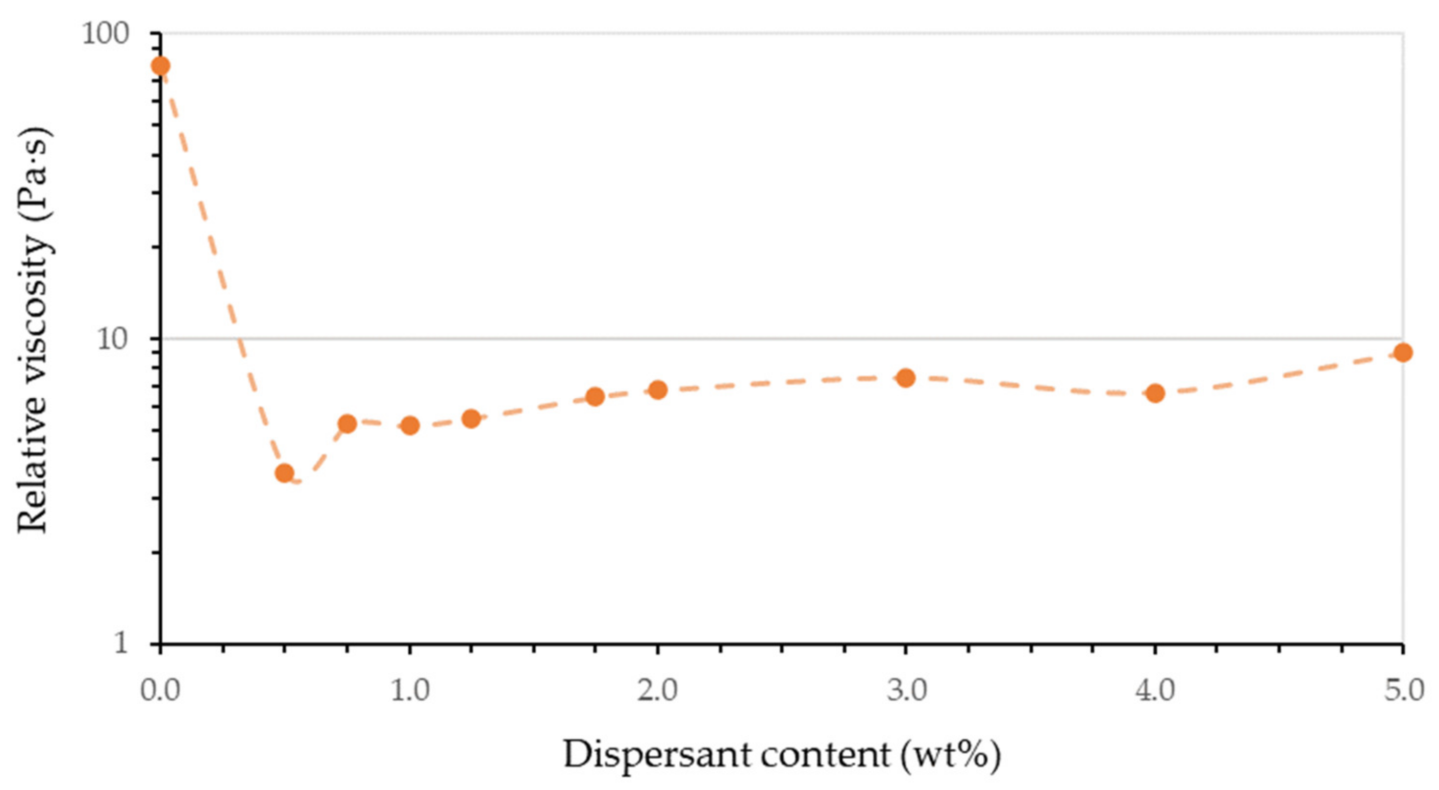
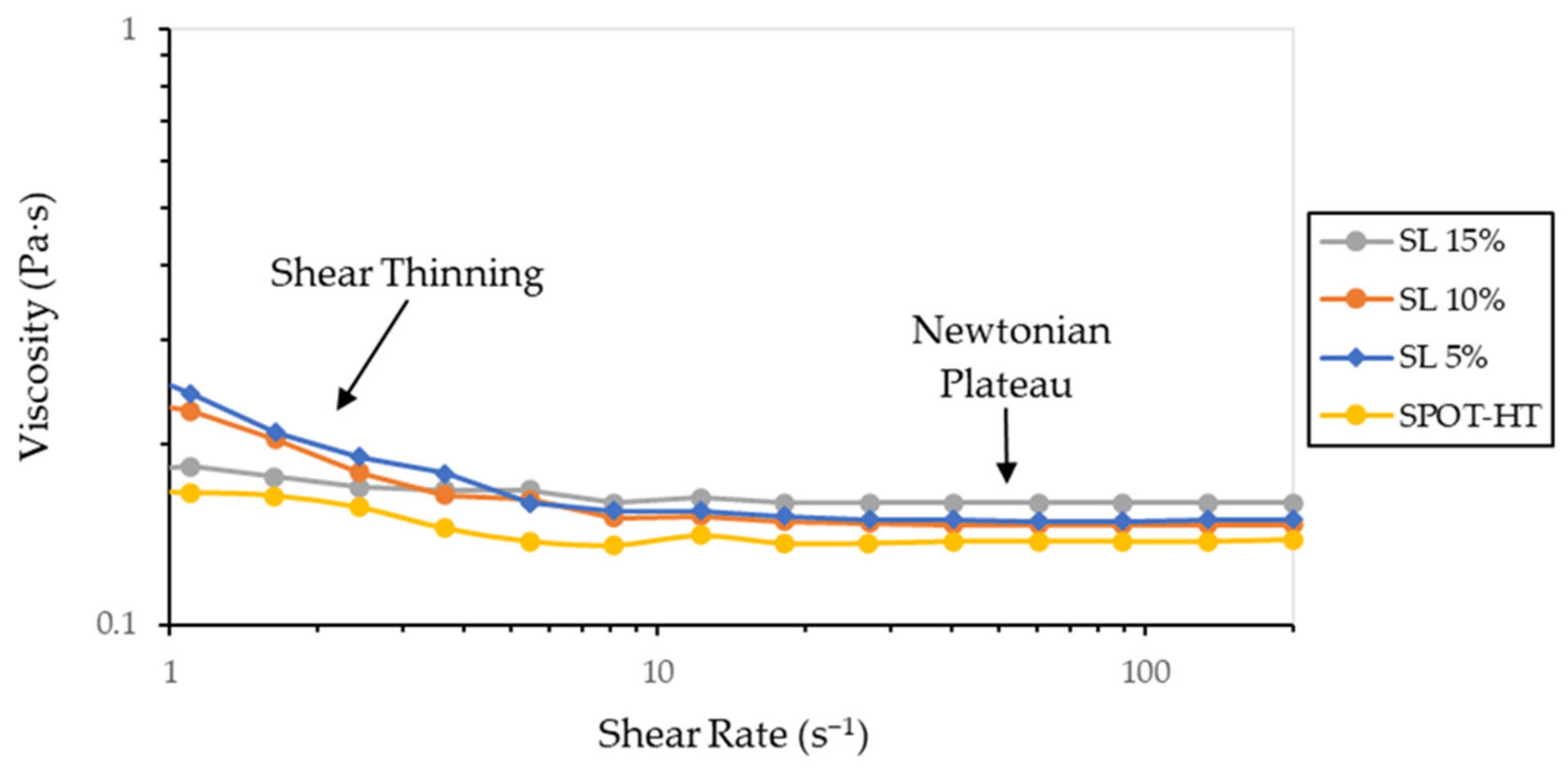
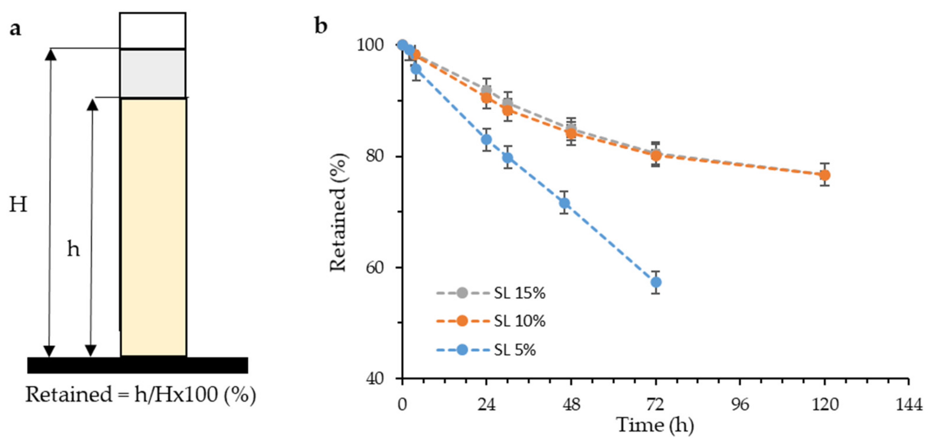
3.1. Characteristics of Reinforced Materials
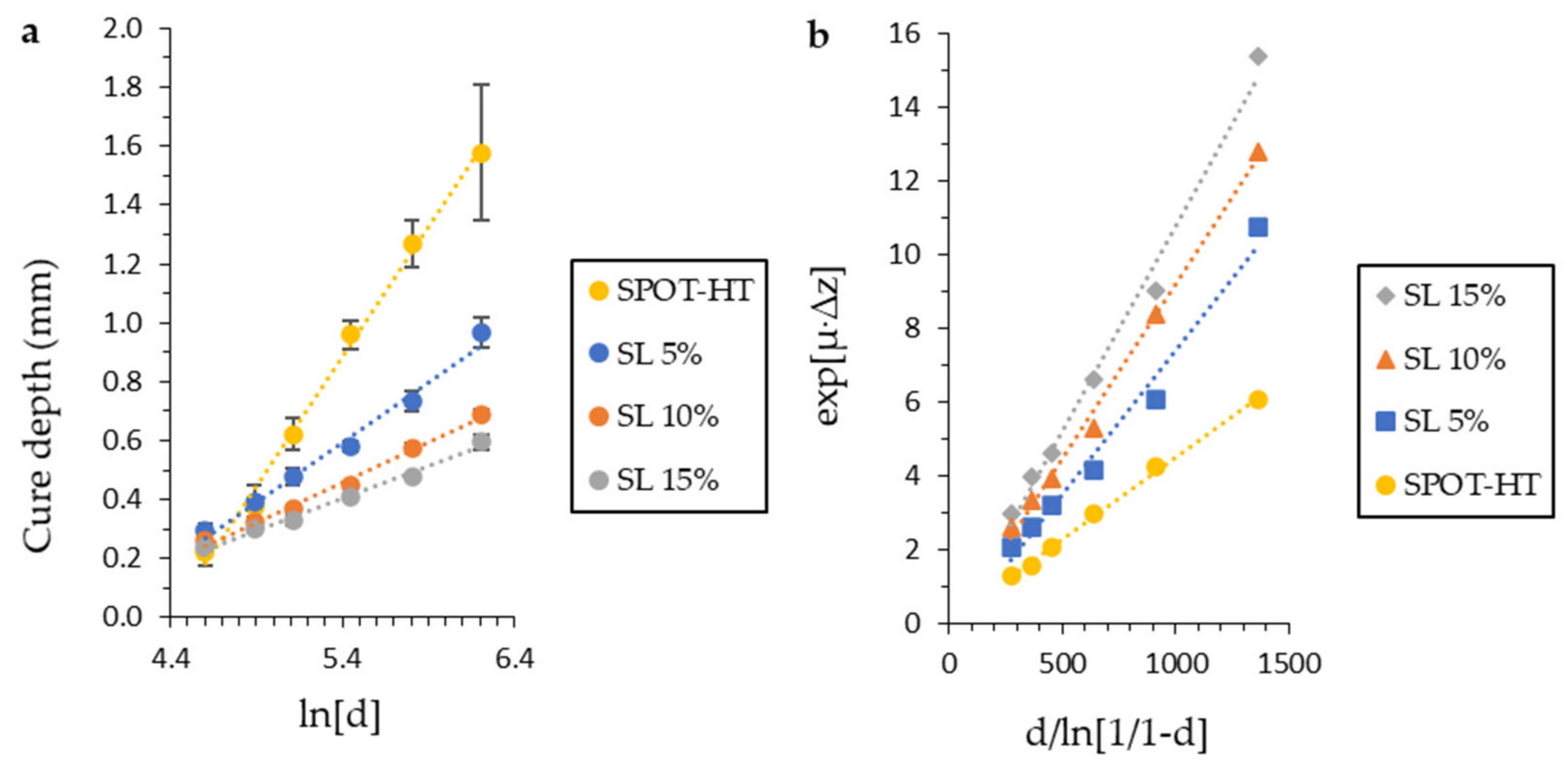
3.2. Definition of Printing Parameters
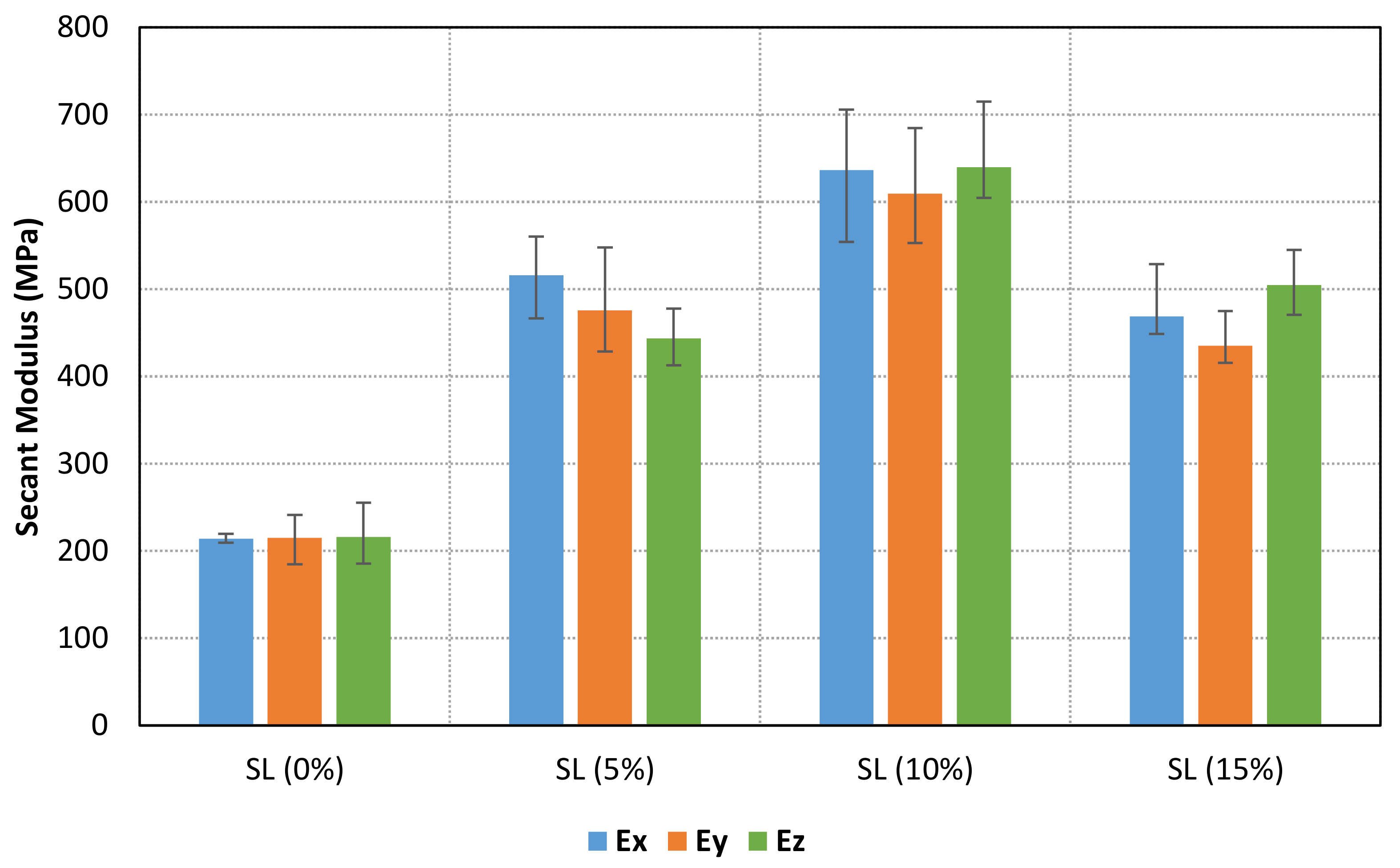
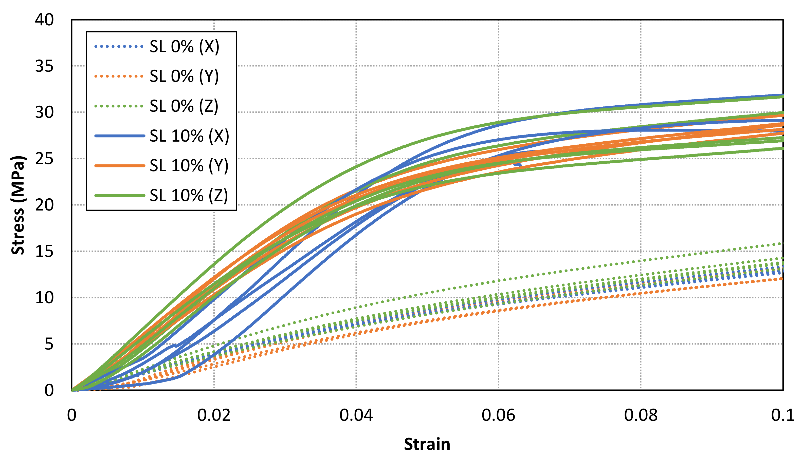
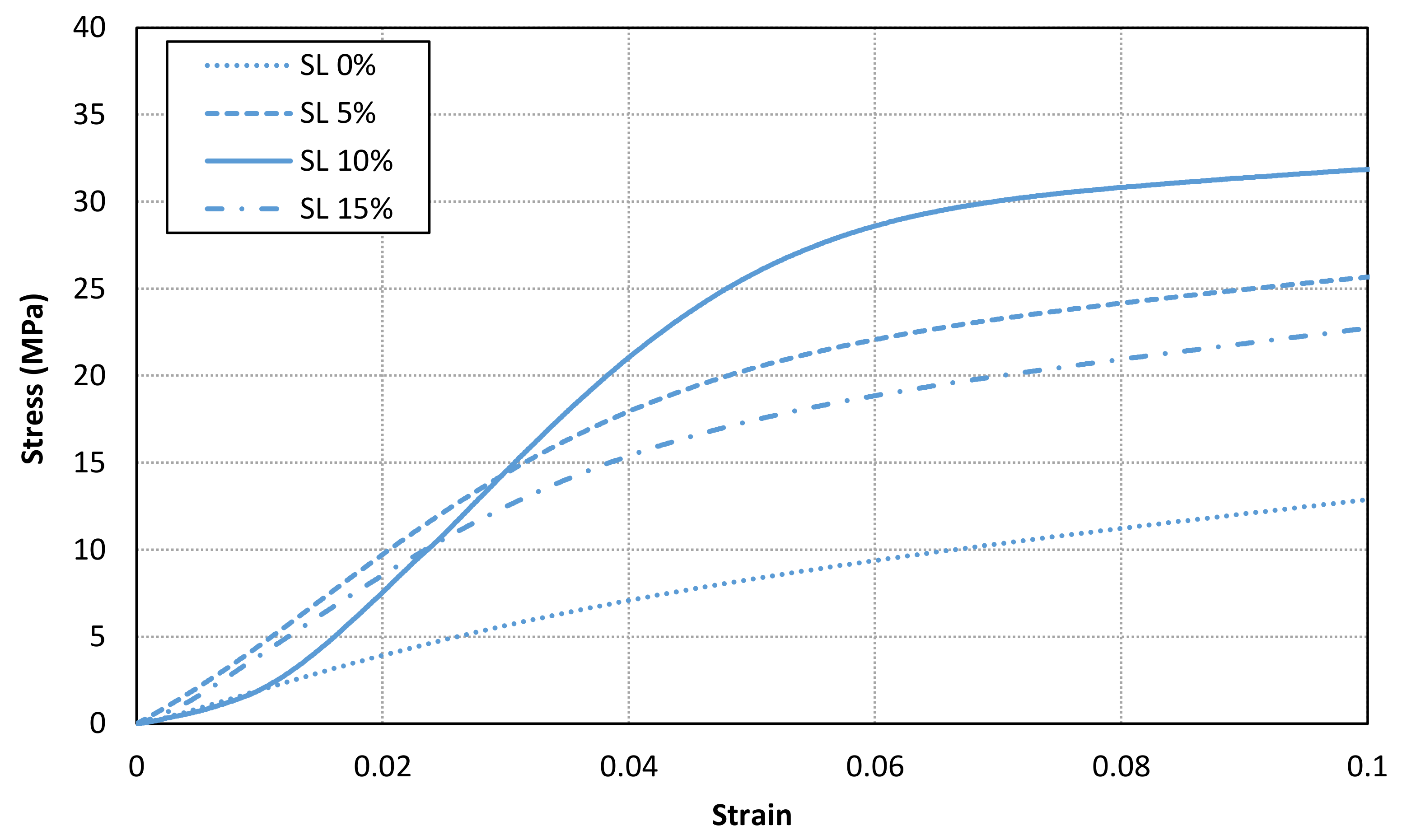
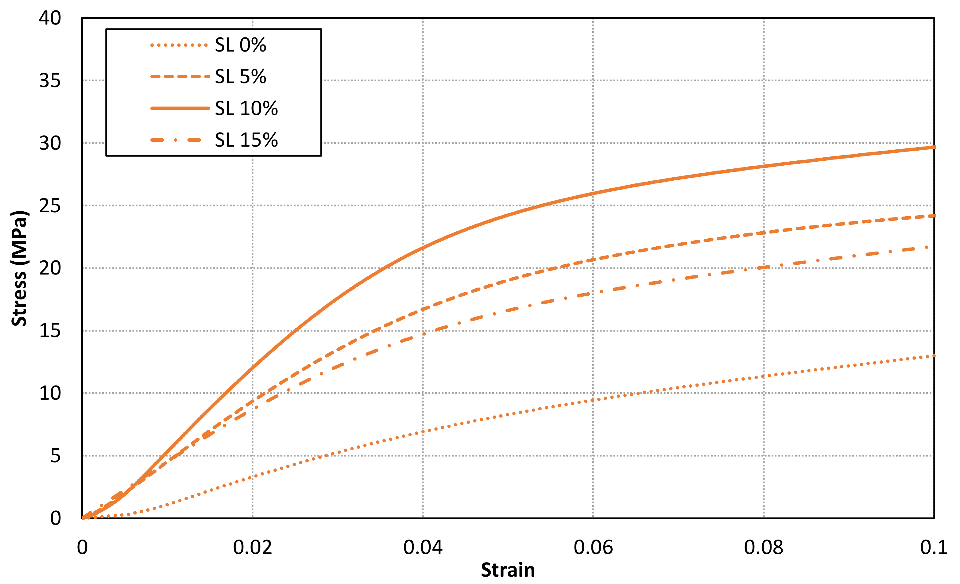
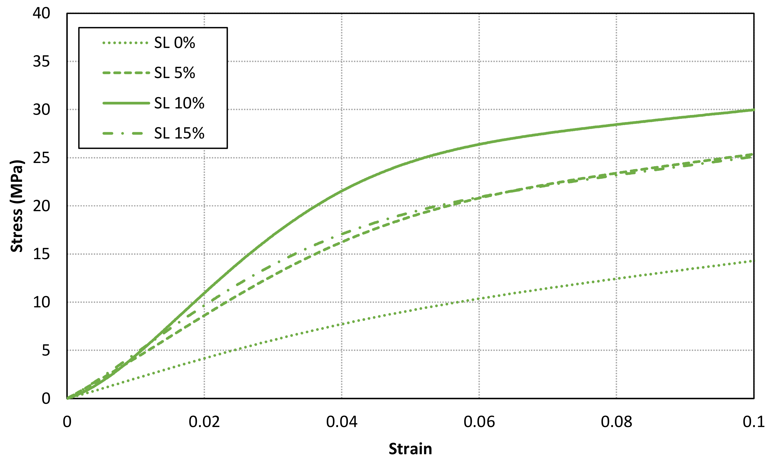
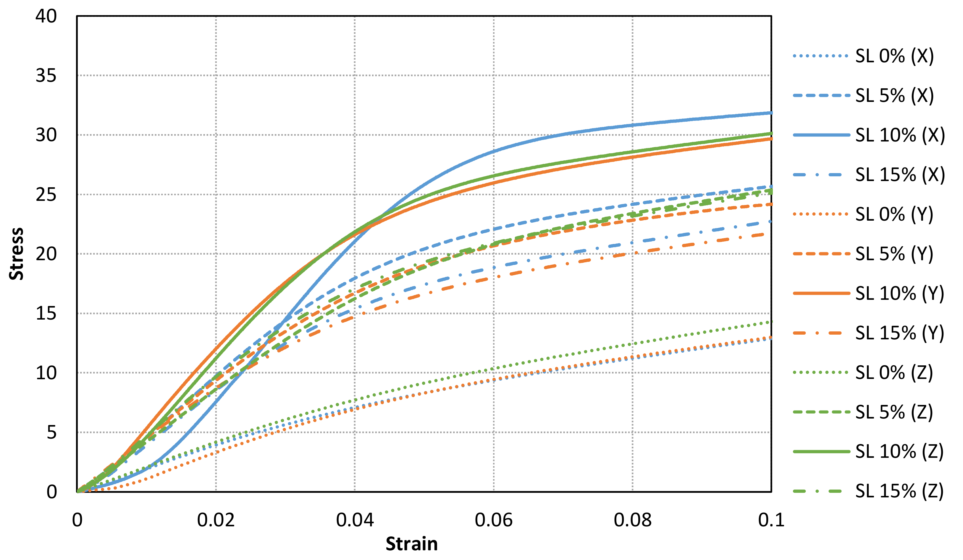
3.3. Analysis of Mechanical Properties
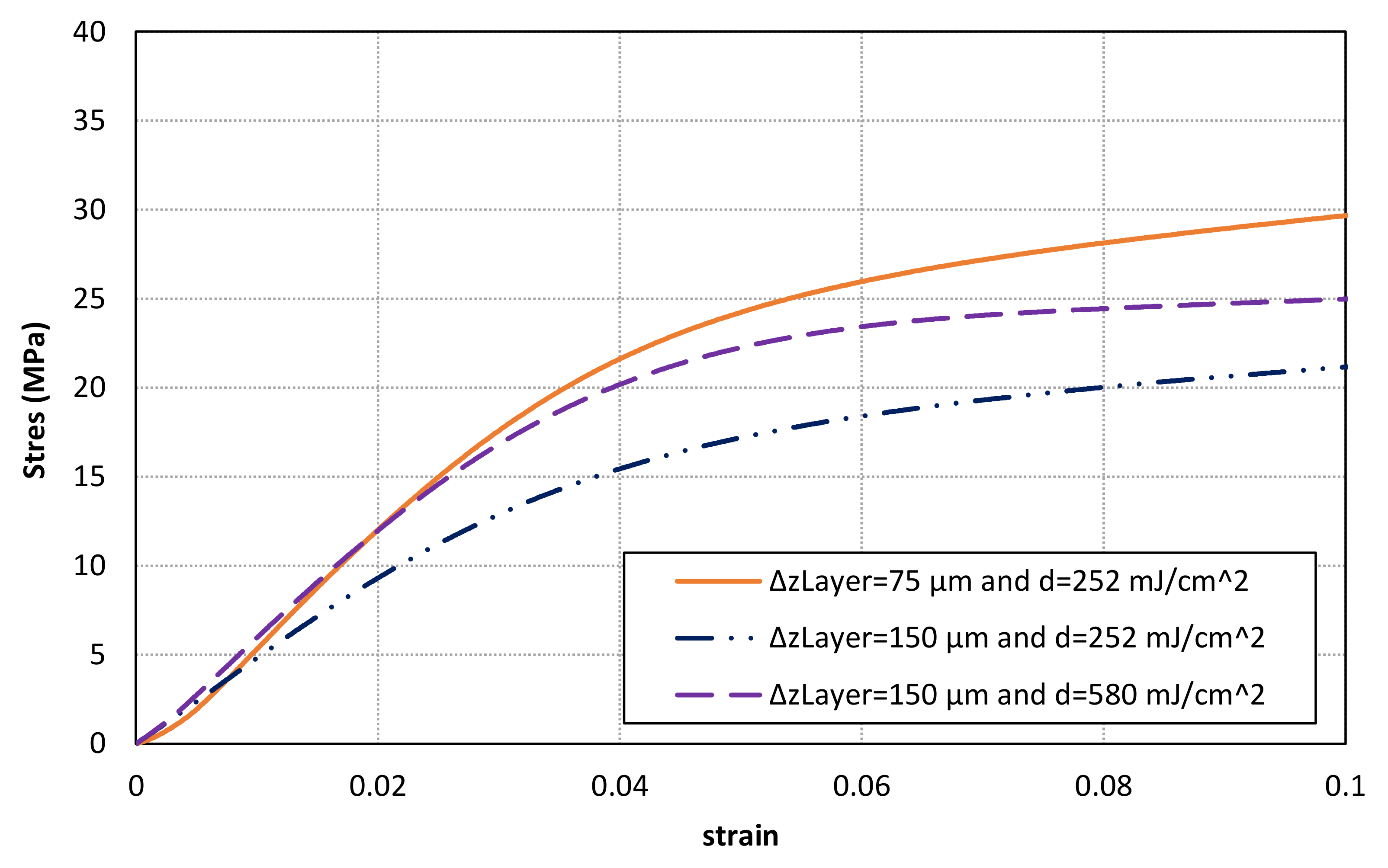
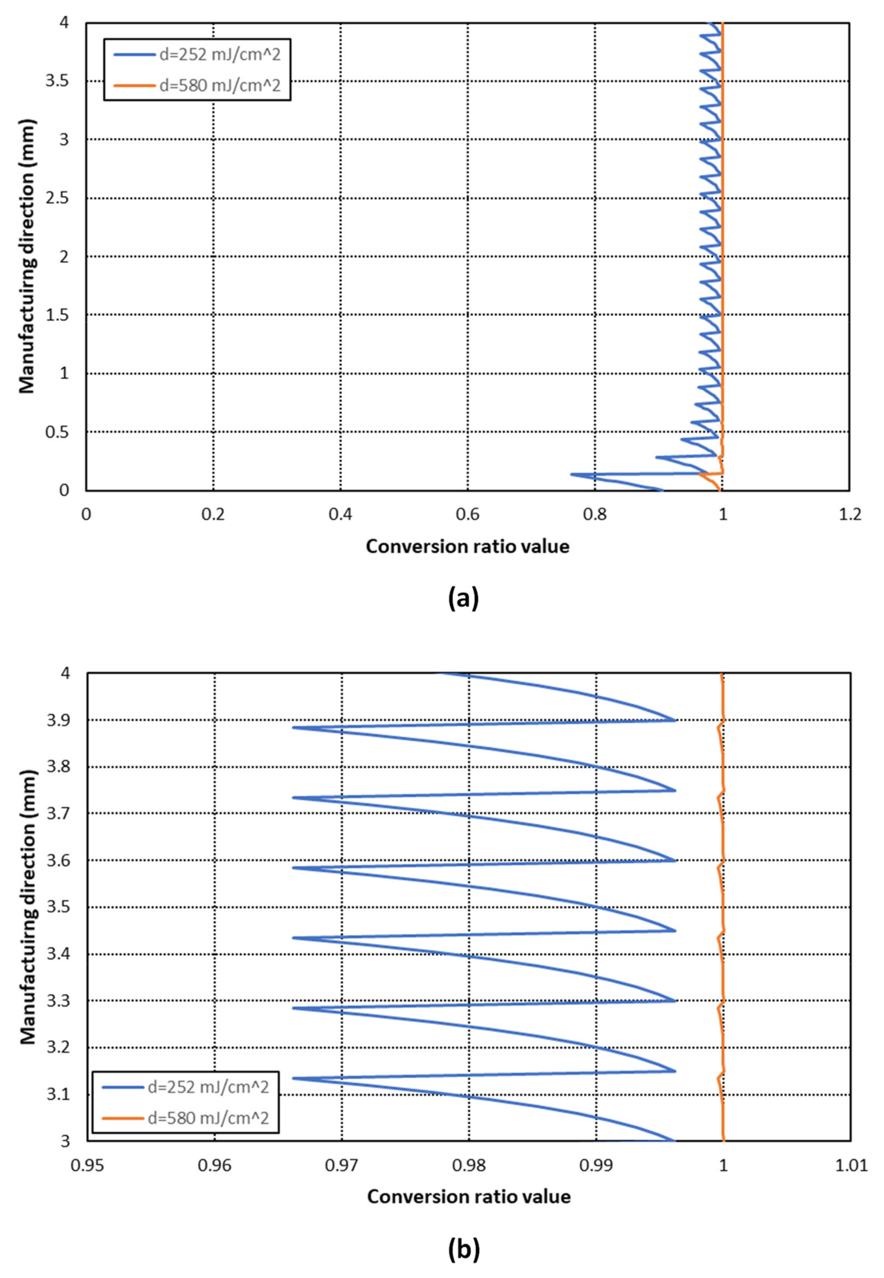
3.4. Optimization of Printing Parameters According to the Layer Thickness
4. Conclusions
Author Contributions
Funding
Institutional Review Board Statement
Informed Consent Statement
Data Availability Statement
Conflicts of Interest
References
- Sun, C.; Fang, N.; Wu, D.; Zhang, X. Projection micro-stereolithography using digital micro-mirror dynamic mask. Sens. Actuators A Phys. 2005, 121, 113–120. [Google Scholar] [CrossRef]
- Limaye, A.S.; Rosen, D.W. Process planning for mask projection stereolithography. Rapid Prototyp. J. 2007, 13, 76–84. [Google Scholar] [CrossRef]
- Vitale, A.; Hennessy, M.; Matar, O.K.; Cabral, J.T. Interfacial Profile and Propagation of Frontal Photopolymerization Waves. Macromolecules 2014, 48, 198–205. [Google Scholar] [CrossRef]
- Bonada, J.; Muguruza, A.; Francos, X.F.; Ramis, X. Influence of exposure time on mechanical properties and photocuring conversion ratios for photosensitive materials used in Additive Manufacturing. Procedia Manuf. 2017, 13, 762–769. [Google Scholar] [CrossRef]
- Bonada, J.; Muguruza, A.; Fernández-Francos, X.; Ramis, X. Optimization procedure for additive manufacturing process based on mask image projection to improve Z accuracy and resolution. J. Manuf. Process. 2018, 31, 689–702. [Google Scholar] [CrossRef] [Green Version]
- Cabral, J.T.; Douglas, J.F. Propagating waves of network formation induced by light. Polymer 2005, 46, 4230–4241. [Google Scholar] [CrossRef]
- Vitale, A.; Cabral, J.T. Frontal Conversion and Uniformity in 3D Printing by Photopolymerisation. Materials 2016, 9, 760. [Google Scholar] [CrossRef]
- Weng, Z.; Zhou, Y.; Lin, W.; Senthil, T.; Wu, L. Structure-property relationship of nano enhanced stereolithography resin for desktop SLA 3D printer. Compos. Part A Appl. Sci. Manuf. 2016, 88, 234–242. [Google Scholar] [CrossRef]
- Kumar, S.; Hofmann, M.; Steinmann, B.; Foster, J.; Weder, C. Reinforcement of Stereolithographic Resins for Rapid Prototyping with Cellulose Nanocrystals. ACS Appl. Mater. Interfaces 2012, 4, 5399–5407. [Google Scholar] [CrossRef] [PubMed]
- Eng, H.; Maleksaeedi, S.; Yu, S.; Choong, Y.Y.C.; Wiria, F.E.; Tan, C.L.C.; Su, P.C.; Wei, J. 3D Stereolithgraphy of polymer composites reinforced with orientated nanoclay. Procedia Manuf. 2017, 216, 1–7. [Google Scholar]
- Mallakpour, S.; Khadem, E. Recent development in the synthesis of polymer nanocomposites based on nano-alumina. Prog. Polym. Sci. 2015, 51, 74–93. [Google Scholar] [CrossRef]
- Bonada, J.; Xuriguera, E.; Muguruza, A.; Gonçalves, J.; Barcelona, P.; Pons, J.; Minguella, J.; Uceda, R. Reinforced photocurable materials for an Additive Manufacturing process based on Mask Image Projection. Procedia Manuf. 2019, 41, 531–538. [Google Scholar] [CrossRef]
- Monzón, M.; Ortega, Z.; Hernández, A.; Paz, R.; Ortega, F. Anisotropy of Photopolymer Parts Made by Digital Light Processing. Materials 2017, 10, 64. [Google Scholar] [CrossRef] [Green Version]
- Dizon, J.R.C.; Espera, A.H.; Chen, Q.; Advincula, R.C. Mechanical characterization of 3D-printed polymers. Addit. Manuf. 2018, 20, 44–67. [Google Scholar] [CrossRef]
- Aznarte, E.; Qureshi, A.J. A study on material-process interaction and optimization for VAT-photopolymerization processes. Rapid Prototyp. J. 2018, 24, 1479–1485. [Google Scholar] [CrossRef]
- Chang, N.-H.; Song, S.-E.; Park, K. Investigation on Anisotropy according to Printing Conditions for Projection Type Photo-polymerization 3D Printing. Polym. Korea 2018, 42, 1040–1045. [Google Scholar] [CrossRef]
- Garcia, E.A.; Ayranci, C.; Queshi, A.J. Material property-manufactuing process optimization for Form 2 vat-photo polymerization 3D printers. J. Manuf. Mater. Process. 2020, 4, 12. [Google Scholar]
- Vitale, A.; Hennessy, M.G.; Matar, O.K.; Cabral, J.T. A Unified Approach for Patterning via Frontal Photopolymerization. Adv. Mater. 2015, 27, 6118–6124. [Google Scholar] [CrossRef] [PubMed]
- Alvankarian, J.; Majlis, B.Y. Exploiting the Oxygen Inhibitory Effect on UV Curing in Microfabrication: A Modified Lithography Technique. PLoS ONE 2015, 10, e0119658. [Google Scholar] [CrossRef] [PubMed] [Green Version]
- ASTM D695-15. Standard Test. Method for Compressive Properties of Rigid Plastics; ASTM International: West Conshohocken, PA, USA, 2015. [Google Scholar]
- Casafont, M.; Pons, J.M.; Bonada, J.; Pastor, M.M.; Marimon, F.; Roure, F. Experimental study of the compression behaviour of mask image projection based on stereolithography manufactured parts. Procedia Manuf. 2019, 41, 460–467. [Google Scholar] [CrossRef]
- Zhang, J.; Wei, L.; Meng, X.; Yu, F.; Yang, N.; Liu, S. Digital light processing-stereolithography three-dimensional printing of yttria-stabilized zirconia. Ceram. Int. 2020, 46, 8745–8753. [Google Scholar] [CrossRef]


| Code | SPOT-HT (wt%) | Alumina (wt%) | Dispersant (wt% 1) | Antifoam (wt%) |
| SL 5% | 94.6 | 5.0 | 0.5 | 0.4 |
| SL 10% | 89.6 | 10.0 | 0.5 | 0.4 |
| SL 15% | 84.6 | 14.9 | 0.5 | 0.4 |
| SL 0% | SL 5% | SL 10% | SL 15% | |
|---|---|---|---|---|
| μ (mm−1) | 1.139 | 2.45 | 3.69 | 4.59 |
| K(cm2/mJ) | 0.0045 | 0.0073 | 0.0094 | 0.0107 |
| d0 (mJ/cm2) | 126 | 227 | 252 | 277 |
| EX (MPa) | |||||||
|---|---|---|---|---|---|---|---|
| SL | S1 | S2 | S3 | S4 | S5 | Mean | St |
| 0% | 219.48 | 210.42 | 217.91 | 209.29 | 212.61 | 213.94 | 4.53 |
| 5% | 540.18 | 466.34 | 560.42 | 519.42 | 493.51 | 515.97 | 37.22 |
| 10% | 705.37 | 674.87 | 553.99 | 586.38 | 661.76 | 636.47 | 63.59 |
| 15% | 528.59 | 448.65 | 461.06 | 454.79 | 450.21 | 468.66 | 33.85 |
| EY (MPa) | |||||||
| SL | S1 | S2 | S3 | S4 | S5 | Mean | St |
| 0% | 241.00 | 229.69 | 223.51 | 184.60 | 196.89 | 215.14 | 23.54 |
| 5% | 458.95 | 495.90 | 547.48 | 428.32 | 447.81 | 475.69 | 47.07 |
| 10% | 684.78 | 552.60 | 644.77 | 576.72 | 626.97 | 609.41 | 53.00 |
| 15% | 474.98 | 473.70 | 420.99 | 415.50 | 453.48 | 434.91 | 28.30 |
| EZ (MPa) | |||||||
| SL | S1 | S2 | S3 | S4 | S5 | Mean | St |
| 0% | 255.02 | 213.95 | 185.61 | 211.49 | 212.41 | 215.70 | 24.92 |
| 5% | 441.14 | 442.05 | 443.19 | 477.44 | 412.45 | 443.25 | 23.04 |
| 10% | 650.36 | 604.43 | 714.72 | 607.68 | 621.36 | 639.71 | 45.68 |
| 15% | 504.41 | 470.35 | 488.02 | 516.63 | 544.94 | 504.87 | 28.37 |
| EZ (MPa) | ||||||||
|---|---|---|---|---|---|---|---|---|
| ΔzLayer (μm) | d (mJ/cm2) | S1 | S2 | S3 | S4 | S5 | Mean | St |
| 75 | 252 | 684.78 | 552.60 | 644.77 | 576.72 | 626.97 | 609.41 | 53.00 |
| 150 | 252 | 450.20 | 485.75 | 464.27 | 507.19 | 450.66 | 471.61 | 24.58 |
| 150 | 580 | 558.73 | 635.36 | 597.11 | 605.00 | 614.69 | 602.18 | 28.19 |
Publisher’s Note: MDPI stays neutral with regard to jurisdictional claims in published maps and institutional affiliations. |
© 2021 by the authors. Licensee MDPI, Basel, Switzerland. This article is an open access article distributed under the terms and conditions of the Creative Commons Attribution (CC BY) license (https://creativecommons.org/licenses/by/4.0/).
Share and Cite
Bonada, J.; Barcelona, P.; Casafont, M.; Pons, J.M.; Padilla, J.A.; Xuriguera, E. Analysis of the Compression Behaviour of Reinforced Photocurable Materials Used in Additive Manufacturing Processes Based on a Mask Image Projection System. Materials 2021, 14, 4605. https://doi.org/10.3390/ma14164605
Bonada J, Barcelona P, Casafont M, Pons JM, Padilla JA, Xuriguera E. Analysis of the Compression Behaviour of Reinforced Photocurable Materials Used in Additive Manufacturing Processes Based on a Mask Image Projection System. Materials. 2021; 14(16):4605. https://doi.org/10.3390/ma14164605
Chicago/Turabian StyleBonada, Jordi, Pol Barcelona, Miquel Casafont, Josep Maria Pons, Jose Antonio Padilla, and Elena Xuriguera. 2021. "Analysis of the Compression Behaviour of Reinforced Photocurable Materials Used in Additive Manufacturing Processes Based on a Mask Image Projection System" Materials 14, no. 16: 4605. https://doi.org/10.3390/ma14164605
APA StyleBonada, J., Barcelona, P., Casafont, M., Pons, J. M., Padilla, J. A., & Xuriguera, E. (2021). Analysis of the Compression Behaviour of Reinforced Photocurable Materials Used in Additive Manufacturing Processes Based on a Mask Image Projection System. Materials, 14(16), 4605. https://doi.org/10.3390/ma14164605