
The Variable Frequency Conductivity of Geopolymers during the Long Agieng Period


Abstract
:1. Introduction
2. Materials and Methods
2.1. Materials and Sample Preparation
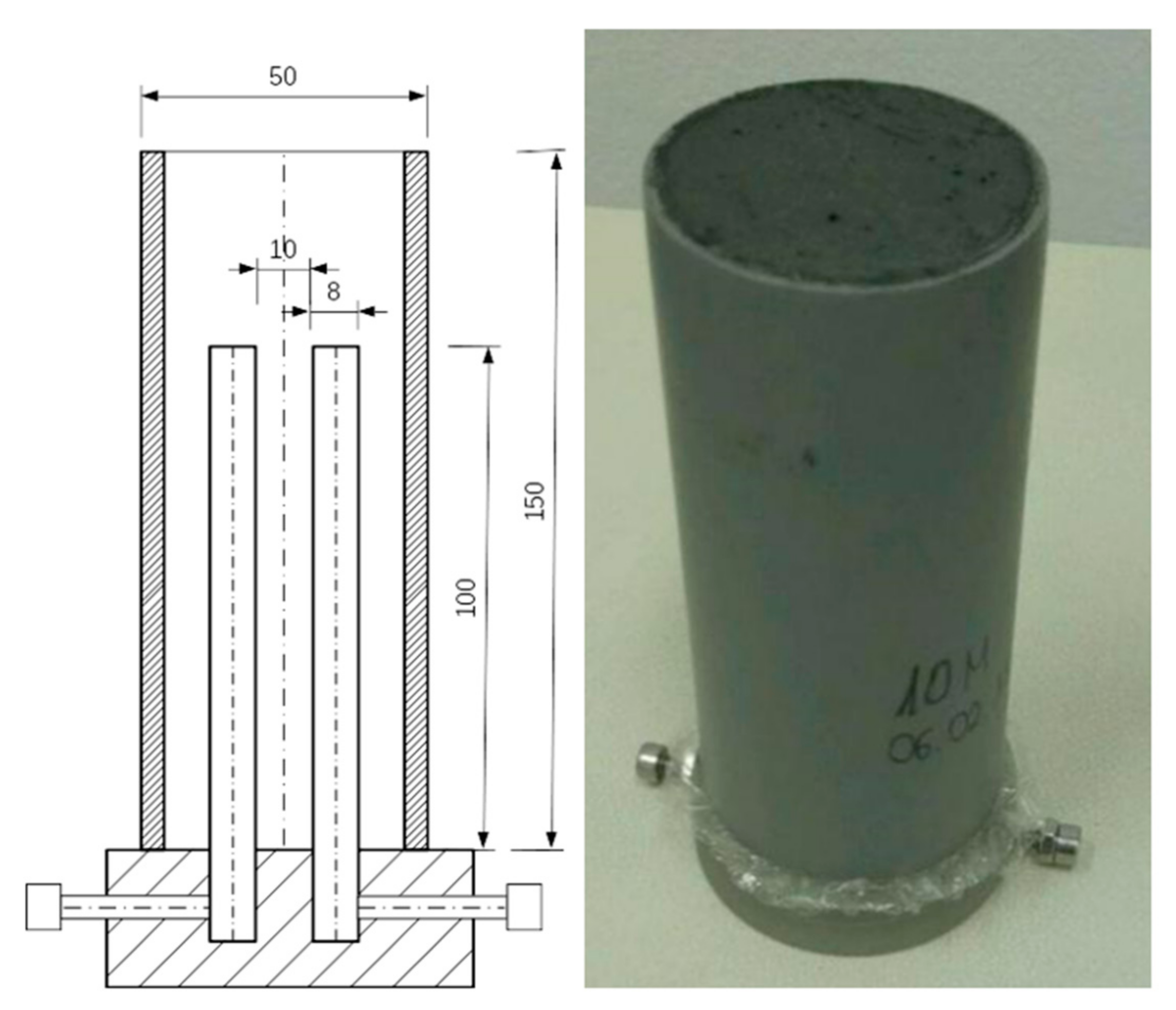
2.2. Conductivity Measurements
2.3. XRD Methods
2.4. Physical Sorption Analysis
2.5. Porosity
3. Results
3.1. Results of Conductivity Measurements
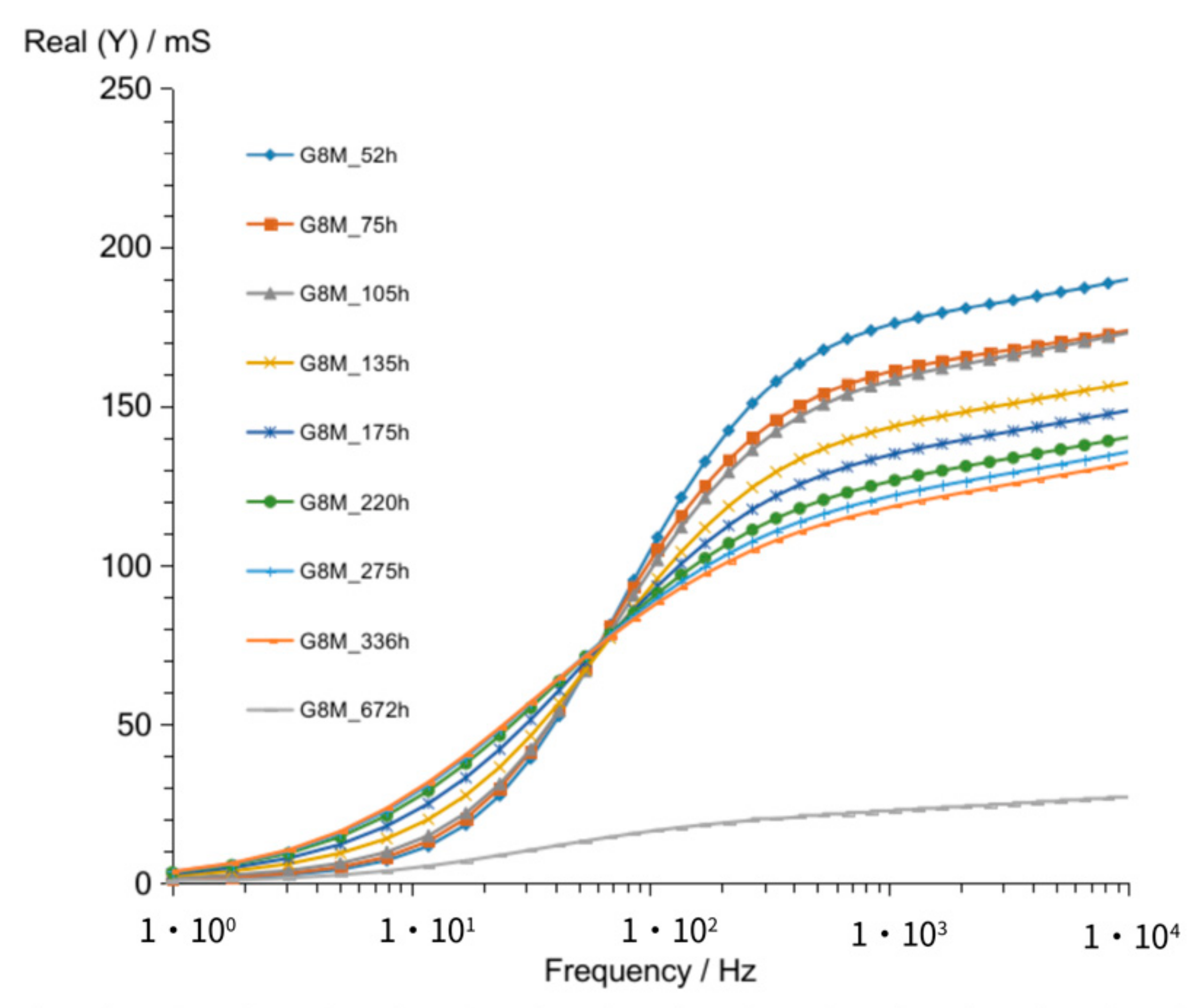
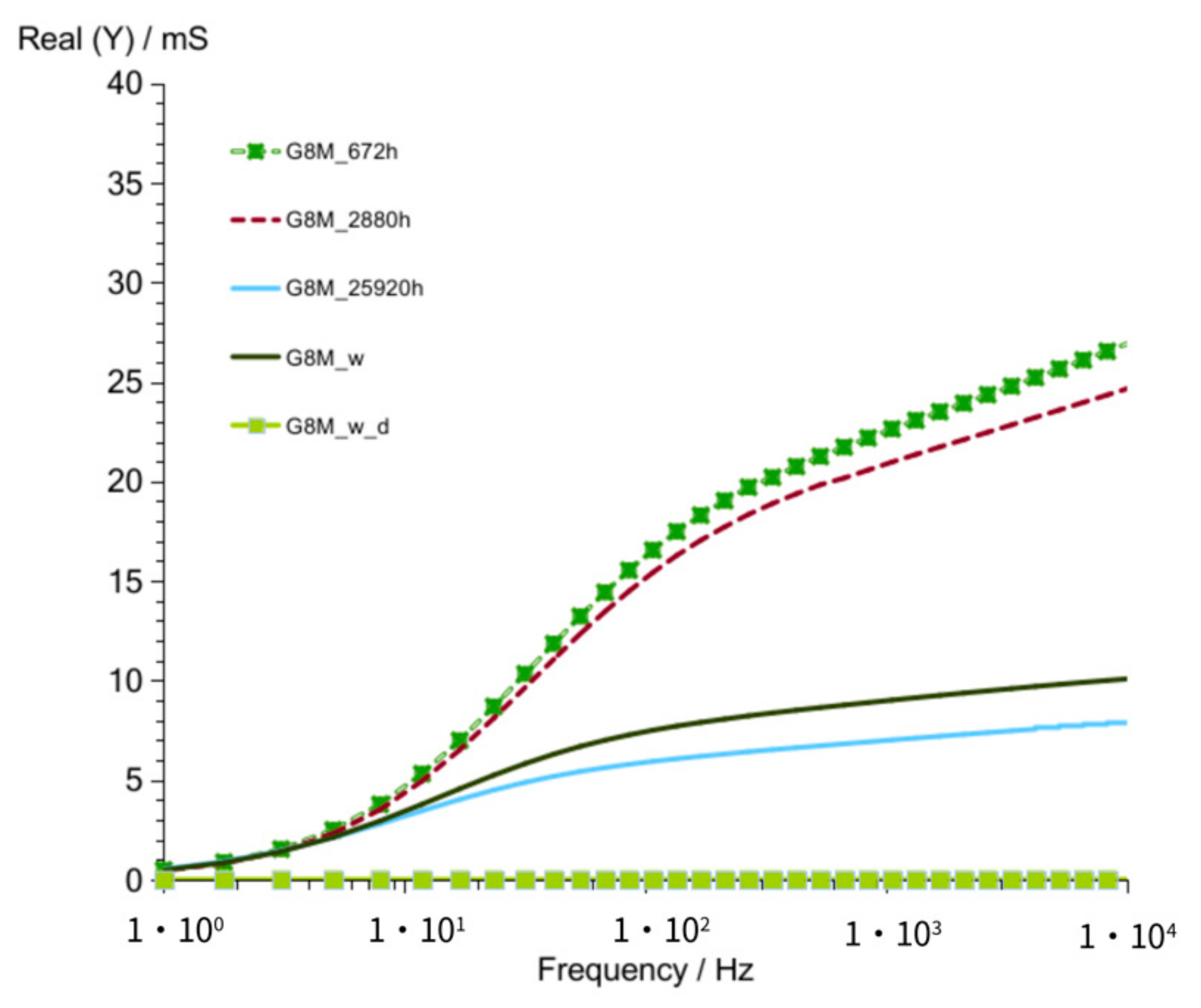
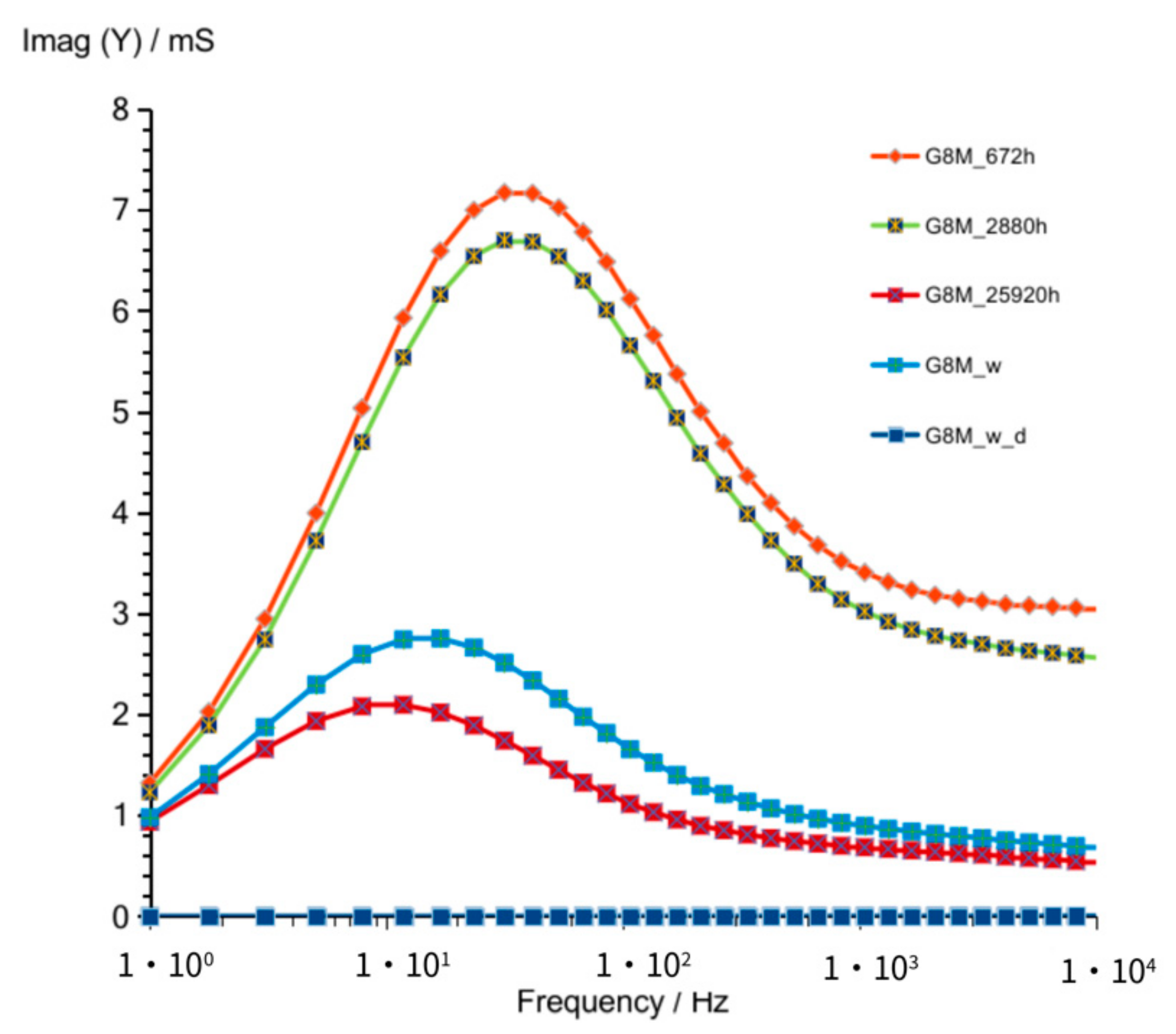
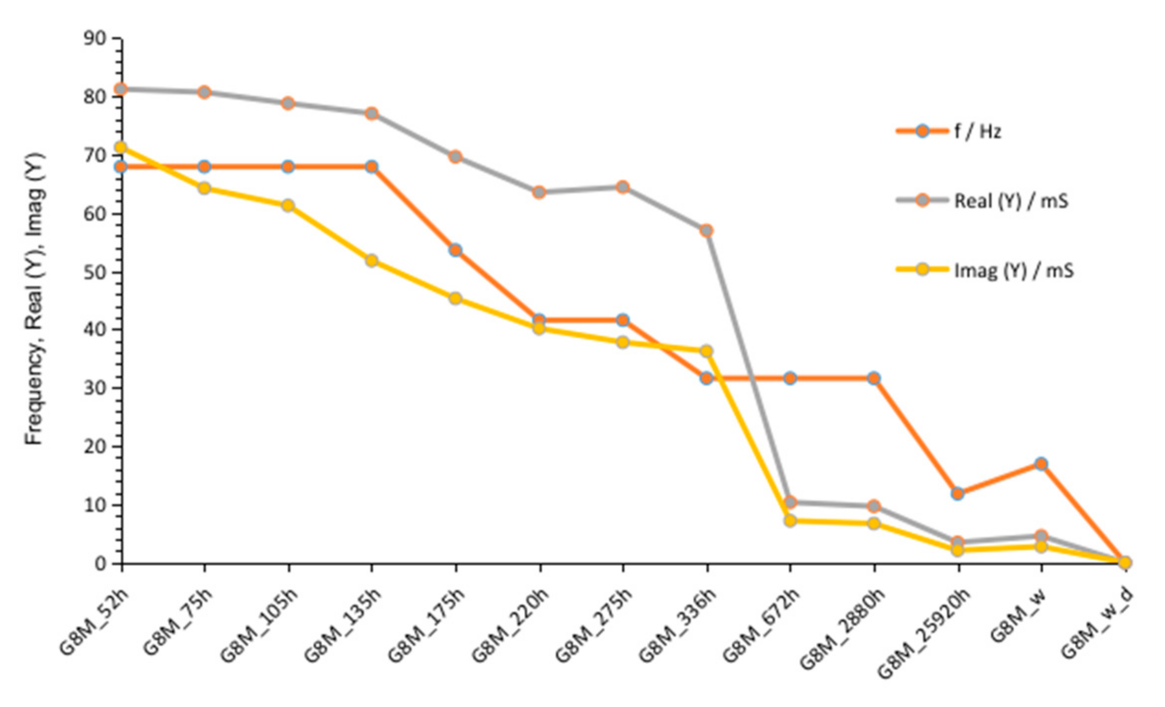
3.1.1. G8M
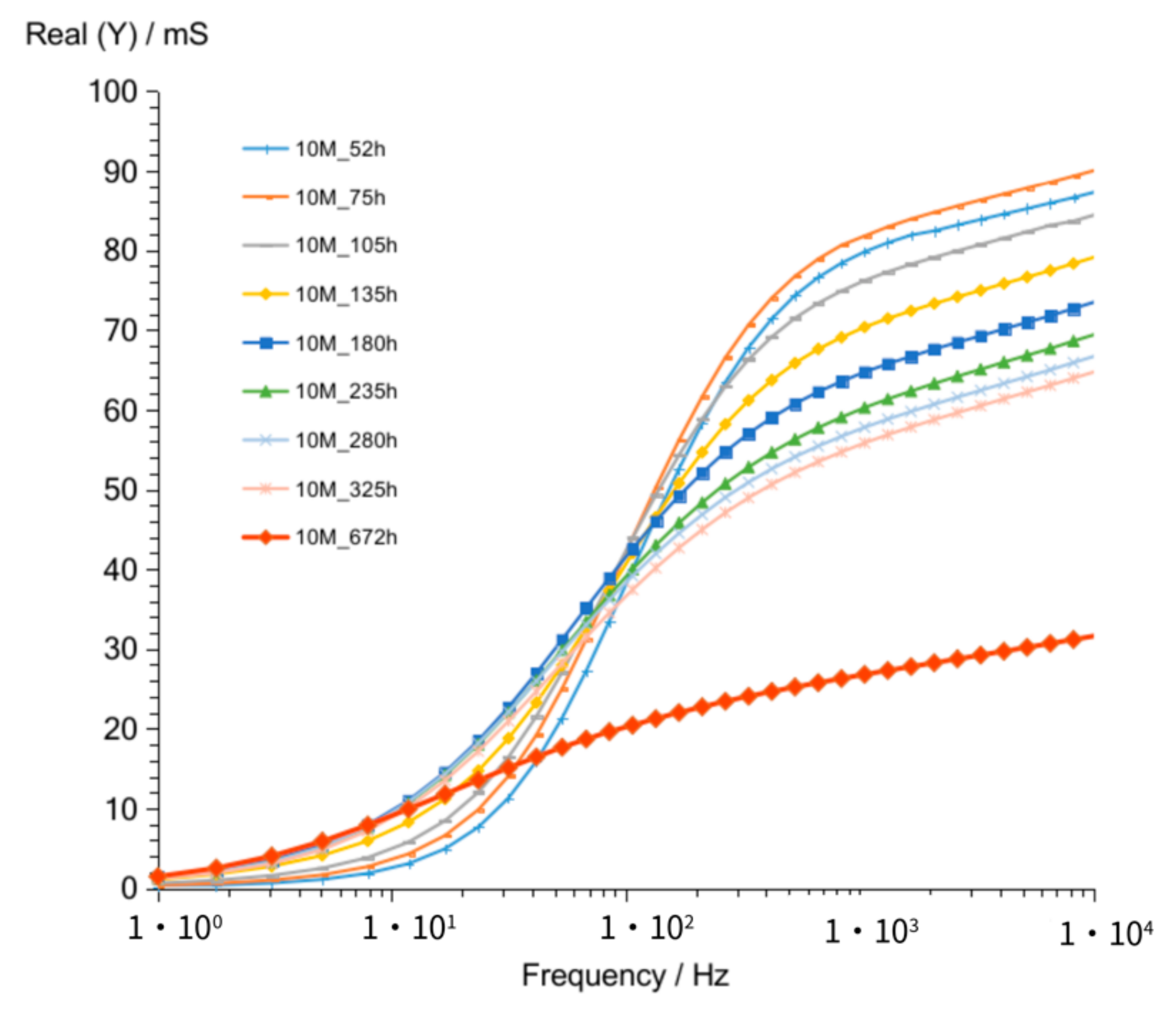
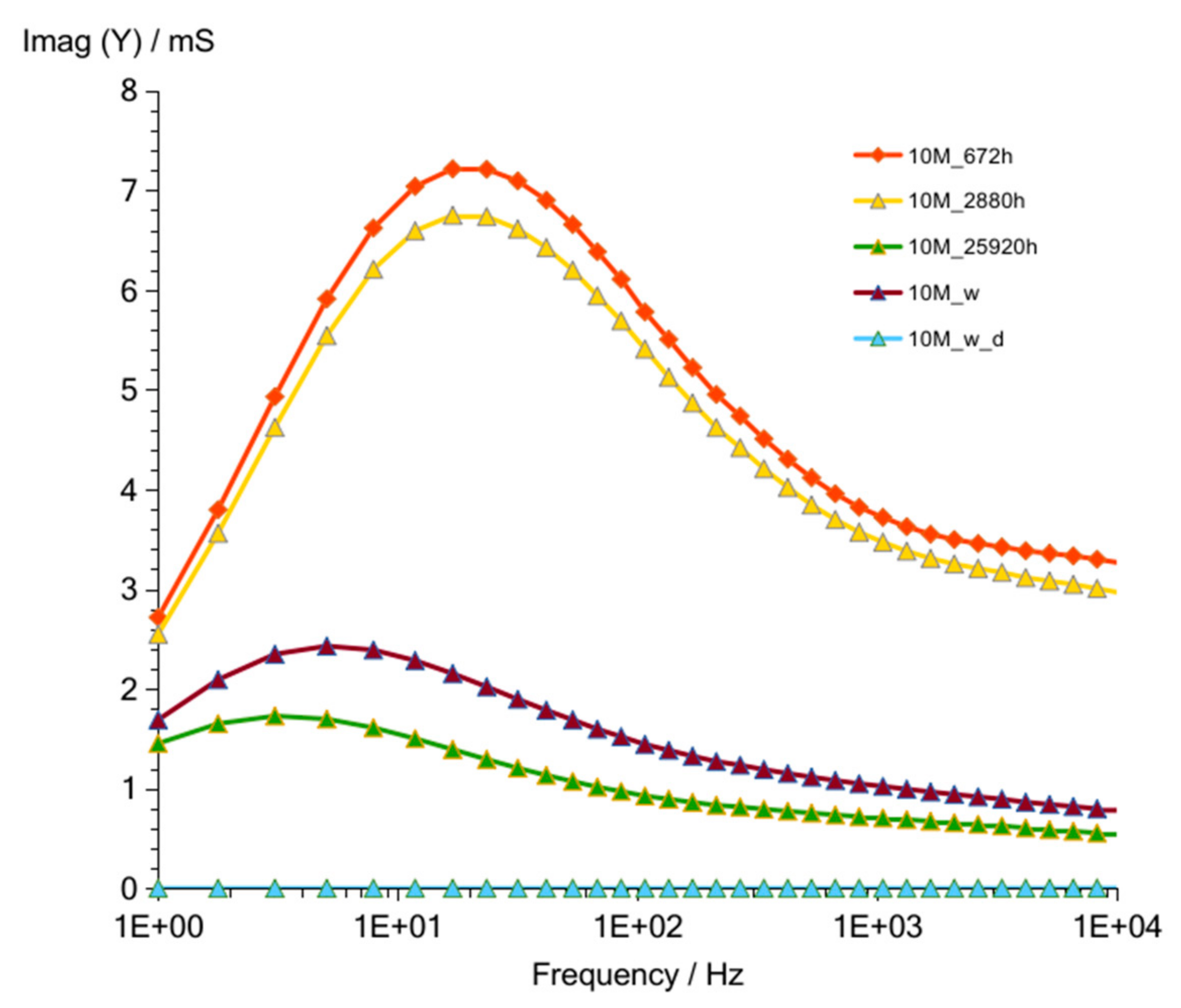
3.1.2. G10M
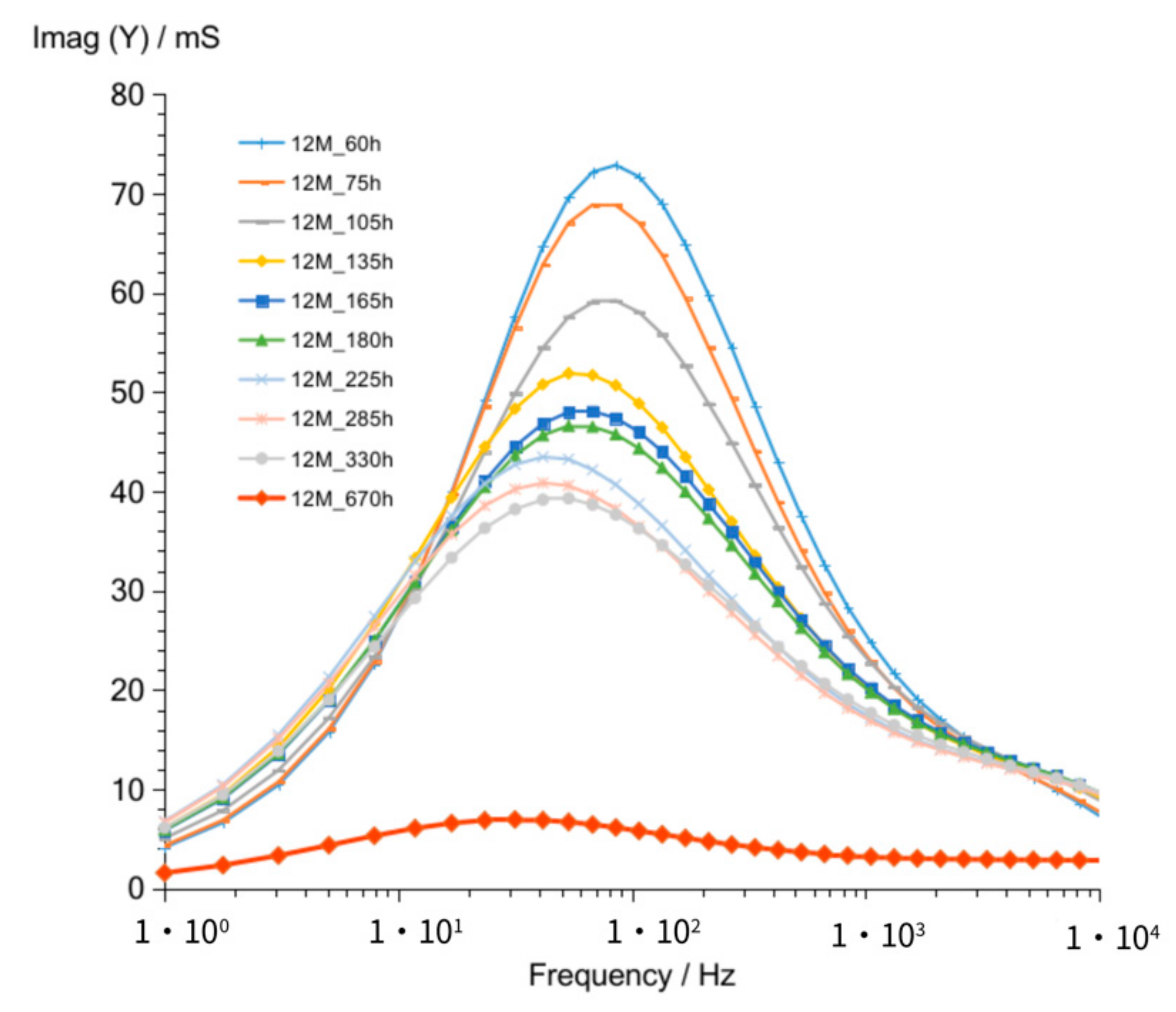
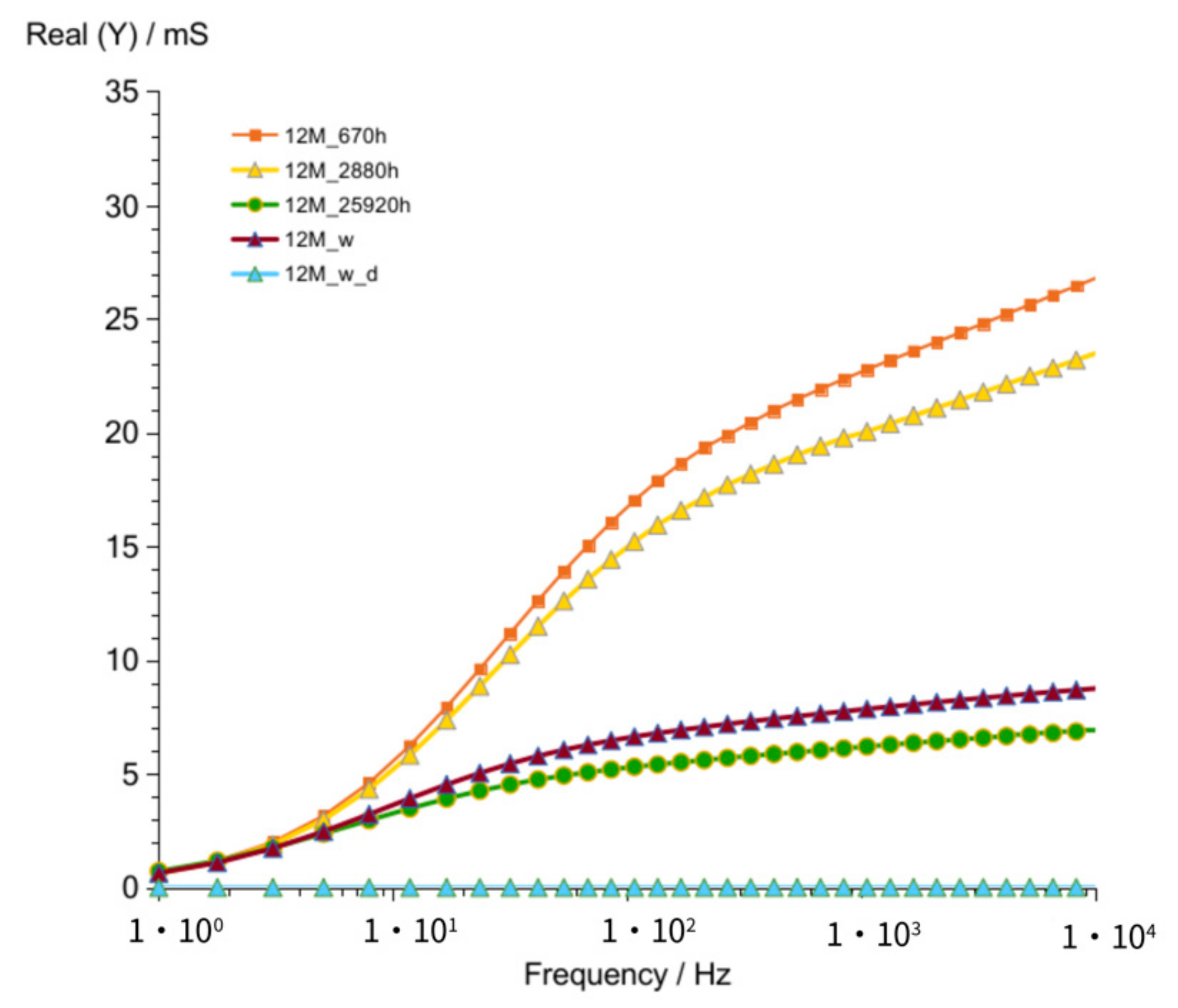
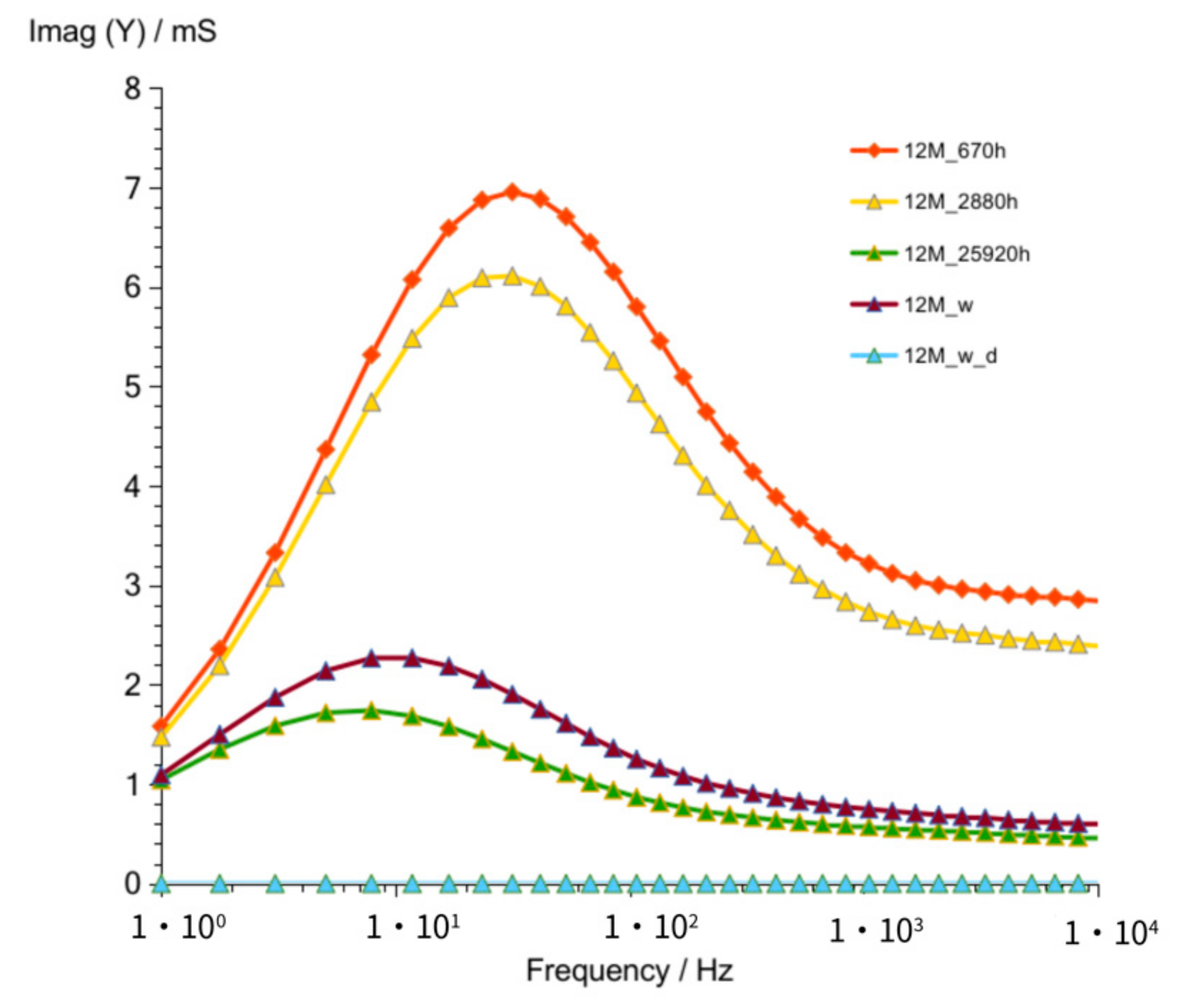
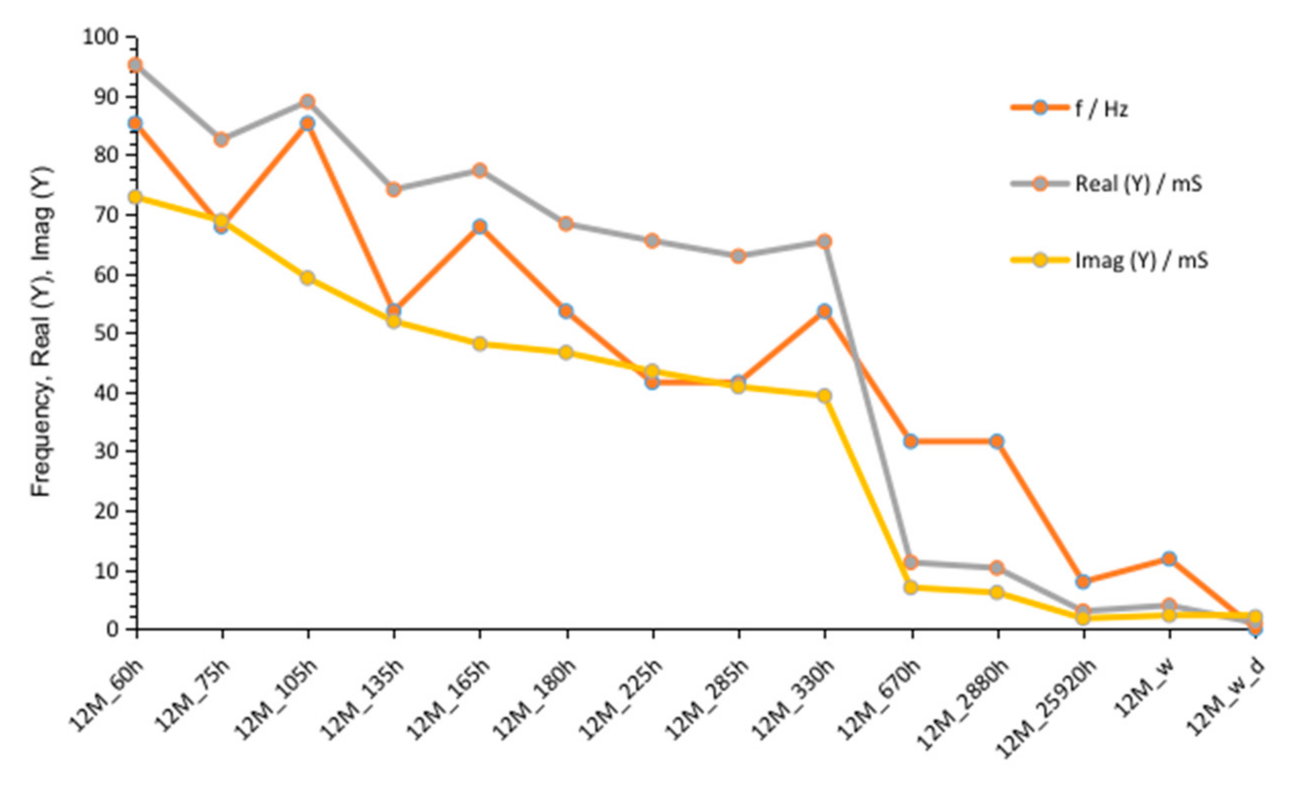
3.1.3. G12M

| Value Describing | G8M | G10M | G12M | |
|---|---|---|---|---|
| Figure 2 Figure 7 Figure 12 | crossing curves frequency—Real (Y) | 68 Hz | 90 Hz | 68 Hz |
| values of Real (Y) at 1 kHz (at time about 60 to 320 h) | 176–118 mS | 82–56 mS | 185–123 mS | |
| values of Imag (Y) at 1 kHz (at time about 60 to 320 h) | 21–13.5 mS | 12–8.3 mS | 24.7–17.7 mS | |
| Figure 3 Figure 8 Figure 13 | frequency of susceptance maximum peak—Imag (Y) (at time about 60 to 320 h) | 70–30 Hz | 100–50 Hz | 90–50 Hz |
| Figure 6 Figure 11 Figure 16 | values of Real (Y) at frequency of susceptance maximum peak (at time about 60 to 320 h) | 68–32 mS | 44–28 mS | 95–65 mS |
| Figure 6 Figure 11 Figure 16 | values of Imag (Y) at frequency of susceptance maximum peak (at time about 60 to 320 h) | 71–36 mS | 33–18 mS | 73–39 mS |
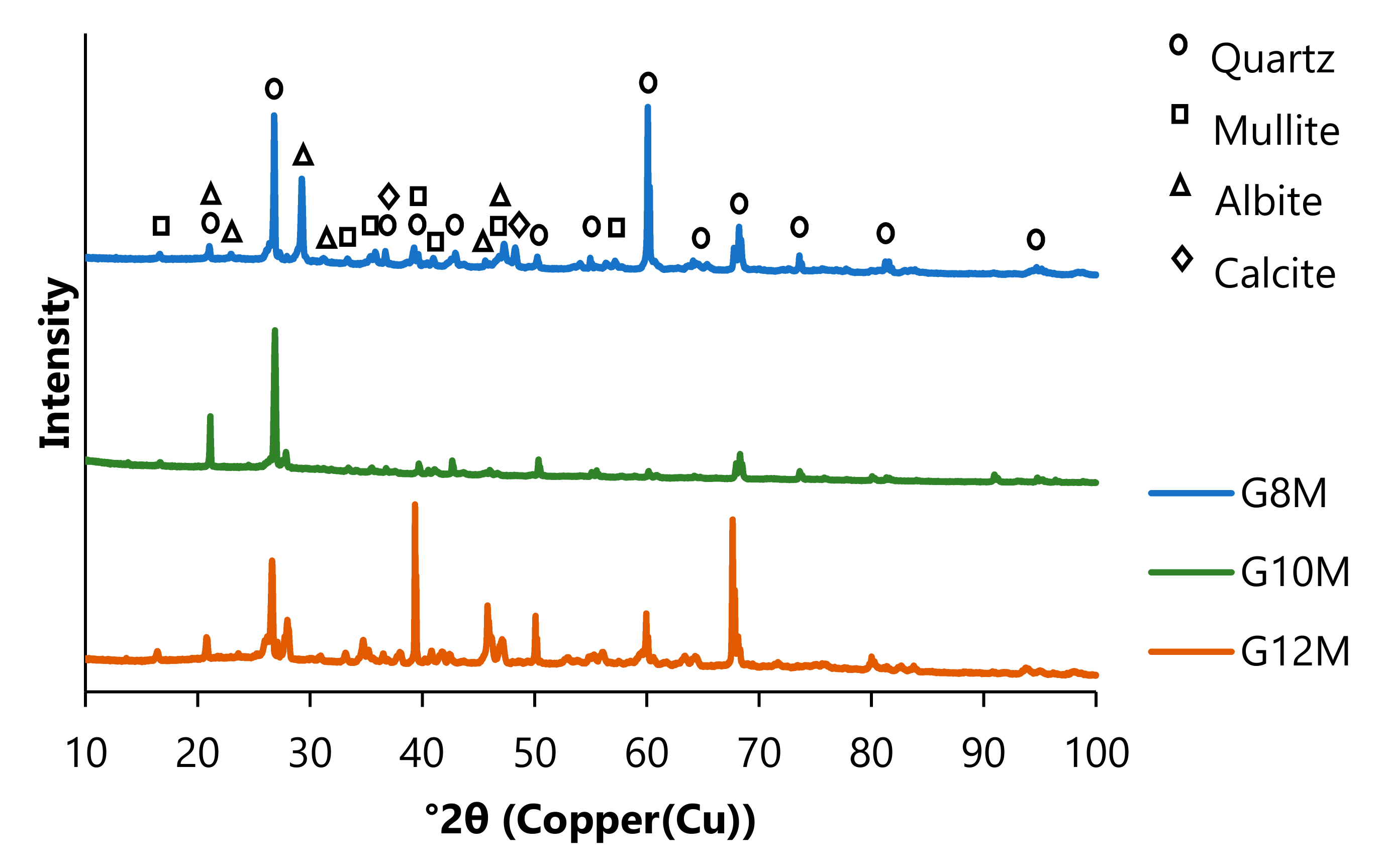
3.2. Results of XRD
3.3. Results of Porosity
3.4. Results of Physical Sorption Analysis
4. Discussion
5. Conclusions
Author Contributions
Funding
Institutional Review Board Statement
Informed Consent Statement
Data Availability Statement
Acknowledgments
Conflicts of Interest
References
- Davidovits, J. GEOPOLYMERS Inorganic Polymerie New Materials. J. Therm. Anal. 1991, 37, 1633–1656. [Google Scholar] [CrossRef]
- Lemougna, P.N.; MacKenzie, K.J.D.; Melo, U.F.C. Synthesis and Thermal Properties of Inorganic Polymers (Geopolymers) for Structural and Refractory Applications from Volcanic Ash. Ceram. Int. 2011, 37, 3011–3018. [Google Scholar] [CrossRef]
- Xu, G.; Shi, X. Characteristics and Applications of Fly Ash as a Sustainable Construction Material: A State-of-the-Art Review. Resour. Conserv. Recycl. 2018, 136, 95–109. [Google Scholar] [CrossRef]
- MacKenzie, K.J.D.; Komphanchai, S.; Vagana, R. Formation of Inorganic Polymers (Geopolymers) from 2:1 Layer Lattice Aluminosilicates. J. Eur. Ceram. Soc. 2008, 28, 177–181. [Google Scholar] [CrossRef]
- Sturm, P.; Gluth, G.J.G.; Brouwers, H.J.H.; Kühne, H.C. Synthesizing One-Part Geopolymers from Rice Husk Ash. Constr. Build. Mater. 2016, 124, 961–966. [Google Scholar] [CrossRef]
- Chindaprasirt, P.; Thaiwitcharoen, S.; Kaewpirom, S.; Rattanasak, U. Controlling Ettringite Formation in FBC Fly Ash Geopolymer Concrete. Cem. Concr. Compos. 2013, 41, 24–28. [Google Scholar] [CrossRef]
- Law, D.W.; Adam, A.A.; Molyneaux, T.K.; Patnaikuni, I.; Wardhono, A. Long Term Durability Properties of Class F Fly Ash Geopolymer Concrete. Mater. Struct. Mater. Constr. 2014, 48, 721–731. [Google Scholar] [CrossRef]
- Nath, P.; Sarker, P.K. Use of OPC to Improve Setting and Early Strength Properties of Low Calcium Fly Ash Geopolymer Concrete Cured at Room Temperature. Cem. Concr. Compos. 2015, 55, 205–214. [Google Scholar] [CrossRef]
- Korniejenko, K.; Halyag, N.P.; Mucsi, G. Fly Ash as a Raw Material for Geopolymerisation-Chemical Composition and Physical Properties. Proc. IOP Conf. Ser. Mater. Sci. Eng. 2019, 706, 012035. [Google Scholar] [CrossRef]
- Kovalchuk, G.; Fernández-Jiménez, A.; Palomo, A. Alkali-Activated Fly Ash. Relationship between Mechanical Strength Gainsand Initial Ash Chemistry. Mater. Constr. 2008, 58, 35–52. [Google Scholar]
- Gluth, G.J.G.; Lehmann, C.; Rübner, K.; Kühne, H.C. Geopolymerization of a Silica Residue from Waste Treatment of Chlorosilane Production. Mater. Struct. Mater. Constr. 2013, 46, 1291–1298. [Google Scholar] [CrossRef]
- Oh, J.E.; Jun, Y.; Jeong, Y. Characterization of Geopolymers from Compositionally and Physically Different Class F Fly Ashes. Cem. Concr. Compos. 2014, 50, 16–26. [Google Scholar] [CrossRef]
- Van Jaarsveld, J.G.S.; van Deventer, J.S.J.; Lukey, G.C. The Characterisation of Source Materials in Fly Ash-Based Geopolymers. Mater. Lett. 2003, 57, 1272–1280. [Google Scholar] [CrossRef]
- Chindaprasirt, P.; Chareerat, T.; Sirivivatnanon, V. Workability and Strength of Coarse High Calcium Fly Ash Geopolymer. Cem. Concr. Compos. 2007, 29, 224–229. [Google Scholar] [CrossRef]
- Sathonsaowaphak, A.; Chindaprasirt, P.; Pimraksa, K. Workability and Strength of Lignite Bottom Ash Geopolymer Mortar. J. Hazard. Mater. 2009, 168, 44–50. [Google Scholar] [CrossRef]
- Diaz, E.I.; Allouche, E.N.; Eklund, S. Factors Affecting the Suitability of Fly Ash as Source Material for Geopolymers. Fuel 2010, 89, 992–996. [Google Scholar] [CrossRef]
- Turner, L.K.; Collins, F.G. Carbon Dioxide Equivalent (CO2-e) Emissions: A Comparison between Geopolymer and OPC Cement Concrete. Constr. Build. Mater. 2013, 43, 125–130. [Google Scholar] [CrossRef]
- Łach, M. Geopolymer Foams—Will They Ever Become a Viable Alternative to Popular Insulation Materials?—A Critical Opinion. Materials 2021, 14, 3568. [Google Scholar] [CrossRef]
- Korniejenko, K.; Łach, M. Geopolymers Reinforced by Short and Long Fibres—Innovative Materials for Additive Manufacturing. Curr. Opin. Chem. Eng. 2020, 28, 167–172. [Google Scholar] [CrossRef]
- Kozub, B.; Bazan, P.; Mierzwiński, D.; Korniejenko, K. Fly-Ash-Based Geopolymers Reinforced by Melamine Fibers. Materials 2021, 14, 400. [Google Scholar] [CrossRef]
- Korniejenko, K.; Łach, M.; Chou, S.Y.; Lin, W.T.; Mikuła, J.; Mierzwiński, D.; Cheng, A.; Hebda, M. A Comparative Study of Mechanical Properties of Fly Ash-Based Geopolymer Made by Casted and 3D Printing Methods. Proc. IOP Conf. Ser. Mater. Sci. Eng. 2019, 660, 012005. [Google Scholar] [CrossRef] [Green Version]
- Walter, J.; Mierzwiński, D.; Kosiba, K. Analysis of the Alkali-Activated Fly Ashes from Electrostatic Precipitators by Impedance Measurements. Proc. IOP Conf. Ser. Mater. Sci. Eng. 2019, 706, 012013. [Google Scholar] [CrossRef]
- Mierzwiński, D.; Walter, J.; Olkiewicz, P. The Influence of Alkaline Activator Concentration on the Apparent Activation Energy of Alkali-Activated Materials. MATEC Web Conf. 2020, 322, 01008. [Google Scholar] [CrossRef]
- Mierzwiński, D.; Walter, J. Autoclaving of Alkali-Activated Materials. Proc. IOP Conf. Ser. Mater. Sci. Eng. 2019, 706, 012012. [Google Scholar] [CrossRef] [Green Version]
- Mikuła, J.; Łach, M.; Mierzwiński, D. Utylization methods of slags and ash from waste incineration plants. Inżynieria Ekol. 2017, 18, 37–46. [Google Scholar] [CrossRef] [Green Version]
- Mierzwiński, D.; Łach, M.; Mikuła, J. Alkaline treatment and immobilization of secondary waste from waste incineration. Inżynieria Ekol. 2017, 18, 102–108. [Google Scholar] [CrossRef]
- Madhavi, T.C.; Annamalai, S. Electrical conductivity of concrete. J. Eng. Appl. Sci. 2016, 11, 5979–5982. [Google Scholar]
- Azarsa, P.; Gupta, R. Electrical Resistivity of Concrete for Durability Evaluation: A Review. Adv. Mater. Sci. Eng. 2017, 2017, 8453095. [Google Scholar] [CrossRef] [Green Version]
- Zulkifli, N.N.I.; Abdullah, M.M.A.B.; Przybył, A.; Pietrusiewicz, P.; Salleh, M.A.A.M.; Aziz, I.H.; Kwiatkowski, D.; Gacek, M.; Gucwa, M.; Chaiprapa, J. Influence of Sintering Temperature of Kaolin, Slag, and Fly Ash Geopolymers on the Microstructure, Phase Analysis, and Electrical Conductivity. Materials 2021, 14, 2213. [Google Scholar] [CrossRef]
- Korniejenko, K.; Mierzwiński, D.; Szabó, R.; Papné Halyag, N.; Louda, P.; Thorhallsson, E.R.; Mucsi, G. The Impact of the Curing Process on the Efflorescence and Mechanical Properties of Basalt Fibre Reinforced Fly Ash-Based Geopolymer Composites. MATEC Web Conf. 2020, 322, 01004. [Google Scholar] [CrossRef]
- Wang, B.; Gupta, R. Correlation of Electrical Conductivity, Compressive Strength, and Permeability of Repair Materials. ACI Mater. J. 2020, 117, 53–63. [Google Scholar] [CrossRef]
- Lai, Z.; Zhao, X.; Tang, R.; Yang, J. Electrical Conductivity-Based Estimation of Unfrozen Water Content in Saturated Saline Frozen Sand. Adv. Civ. Eng. 2021, 2021, 8881304. [Google Scholar] [CrossRef]
- Cosoli, G.; Mobili, A.; Tittarelli, F.; Revel, G.M.; Chiariotti, P. Electrical Resistivity and Electrical Impedance Measurement in Mortar and Concrete Elements: A Systematic Review. Appl. Sci. 2020, 10, 9152. [Google Scholar] [CrossRef]
- Heifetz, A.; Shribak, D.; Bakhtiari, S.; Aranson, I.S.; Bentivegna, A.F. Qualification of 3-D Printed Mortar with Electrical Conductivity Measurements. IEEE Trans. Instrum. Meas. 2021, 70, 6006108. [Google Scholar] [CrossRef]
- Yakovlev, G.; Vít, Č.; Polyanskikh, I.; Gordina, A.; Pudov, I.; Gumenyuk, A.; Smirnova, O. The Effect of Complex Modification on the Impedance of Cement Matrices. Materials 2021, 14, 557. [Google Scholar] [CrossRef] [PubMed]
- Parsian, H.; Tadayon, M.; Mostofinejad, D.; Avatefi, F. Experimental Study on Correlation between Resistivity Measurement Methods in Concrete. ACI Mater. J. 2018, 115, 33–45. [Google Scholar] [CrossRef]
- Mizerová, C.; Kusák, I.; Rovnaník, P. Electrical properties of fly ash geopolymer composites with graphite conductive admixtures. Acta Polytech. CTU Proc. 2019, 22, 72–76. [Google Scholar] [CrossRef]


| Oxide Composition [wt%] | ||||||||
|---|---|---|---|---|---|---|---|---|
| SiO2 | Al2O3 | Fe2O3 | K2O | CaO | MgO | TiO2 | P2O2 | Na2O |
| 55.89 | 23.49 | 5.92 | 3.55 | 2.72 | 2.61 | 1.09 | 0.82 | 0.59 |
| Sample No. | Aqueous NaOH [mL] + Aqueous Sodium Silicate (Water Glass) [mL] | Fly Ash [g] | Sand [g] |
|---|---|---|---|
| G8M | 120 + 120 | 1000 | 1000 |
| G10M | 120 + 120 | 1000 | 1000 |
| G12M | 120 + 120 | 1000 | 1000 |
| Parameters | Components |
|---|---|
| Angular range: 9.999 ÷ 100°2Ѳ | Nickel filter on the lamp |
| Measuring step: 0.0027166°2Ѳ | 13 mm mask |
| Counting time: 340,425 s | Slot 1° |
| Total measurement time: 13:02:32 | Blade in low position |
| Temperature [°C] | Heating Speed [°/min] | Time of Degassing [min] |
|---|---|---|
| 80 | 2 | 30 |
| 120 | 2 | 30 |
| 350 | 5 | 300 |
| Sample No. | Percentage [%] | |||
|---|---|---|---|---|
| Quartz SiO2 ICDD PDF 01-070-3755 | Mullite Al6Si2O13 ICDD PDF 00-015-0776 | Albite NaAlSi3O8 ICDD PDF 01-080-3255 | Calcite CaCO3 ICDD PDF 00-003-0596 | |
| G8M | 32.3 | 24.5 | 42.2 | 1.1 |
| G10M | 54.8 | 18.3 | 26.8 | 0.1 |
| G12M | 37.0 | 24.2 | 38.0 | 0.7 |
| Sample No. | Total Porosity [%] | Interparticle Porosity [%] | Intraparticle Porosity [%] | Mercury Intrusion Porosity [%] | Pore Tortuosity | Solid Compressibility [m/N] |
|---|---|---|---|---|---|---|
| G8M | 29.8338 | 23.4095 | 6.4243 | 29.8338 | 1.8929 | 1.2476 × 10⁻¹⁰ |
| G10M | 12.3247 | 3.1909 | 9.1338 | 12.3247 | 2.0907 | 6.9597 × 10⁻¹¹ |
| G12M | 9.0900 | 0.6878 | 8.4022 | 9.0900 | 2.1273 | 9.6314 × 10⁻¹¹ |
| Sample No. | Specific Surface Area [m2/g] | Pore Volume [cm3/g] | Pore Size [nm] | |||||
|---|---|---|---|---|---|---|---|---|
| BET One-Point Method | BET Multi-Point Method | Total Pore Volume at a Single Point (P/P0 = 0.95) | BJH Pore Volume | DR Pore Volume | Average Pore Diameter | BJH Average Pore Diameter | DR Average Pore Diameter | |
| G8M | 8.485 | 9.531 | 0.02640 | 0.02507 | 0.00325 | 11.08 | 17.429 | 1.636 |
| G10M | 10.541 | 11.628 | 0.03204 | 0.03077 | 0.00409 | 11.02 | 12.325 | 1.676 |
| G12M | 8.385 | 9.464 | 0.02382 | 0.02382 | 0.02289 | 10.07 | 12.368 | 1.763 |
Publisher’s Note: MDPI stays neutral with regard to jurisdictional claims in published maps and institutional affiliations. |
© 2021 by the authors. Licensee MDPI, Basel, Switzerland. This article is an open access article distributed under the terms and conditions of the Creative Commons Attribution (CC BY) license (https://creativecommons.org/licenses/by/4.0/).
Share and Cite
Walter, J.; Uthayakumar, M.; Balamurugan, P.; Mierzwiński, D. The Variable Frequency Conductivity of Geopolymers during the Long Agieng Period. Materials 2021, 14, 5648. https://doi.org/10.3390/ma14195648
Walter J, Uthayakumar M, Balamurugan P, Mierzwiński D. The Variable Frequency Conductivity of Geopolymers during the Long Agieng Period. Materials. 2021; 14(19):5648. https://doi.org/10.3390/ma14195648
Chicago/Turabian StyleWalter, Janusz, Marimuthu Uthayakumar, Ponnambalam Balamurugan, and Dariusz Mierzwiński. 2021. "The Variable Frequency Conductivity of Geopolymers during the Long Agieng Period" Materials 14, no. 19: 5648. https://doi.org/10.3390/ma14195648