
Enhancing the Accuracy of Linear Finite Element Models of Vehicle Structures Considering Spot-Welded Flanges


Abstract
:1. Introduction
2. Materials and Methods
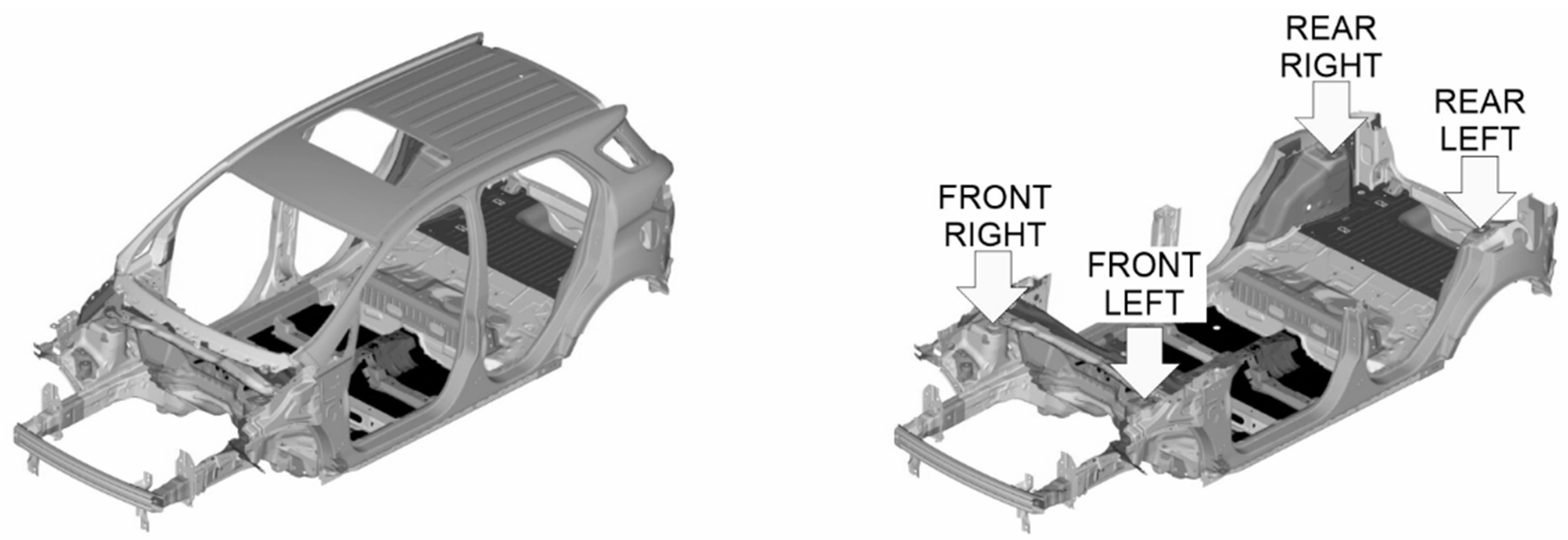
2.1. Tests Performed on the Bench Test. Reference Data
2.1.1. Test Definition
2.1.2. Eigenfrequencies
2.2. Reference FE Model of the Vehicle Body Structure
2.2.1. Model Definition
2.2.2. MAC Matrices
2.2.3. FRAC Results
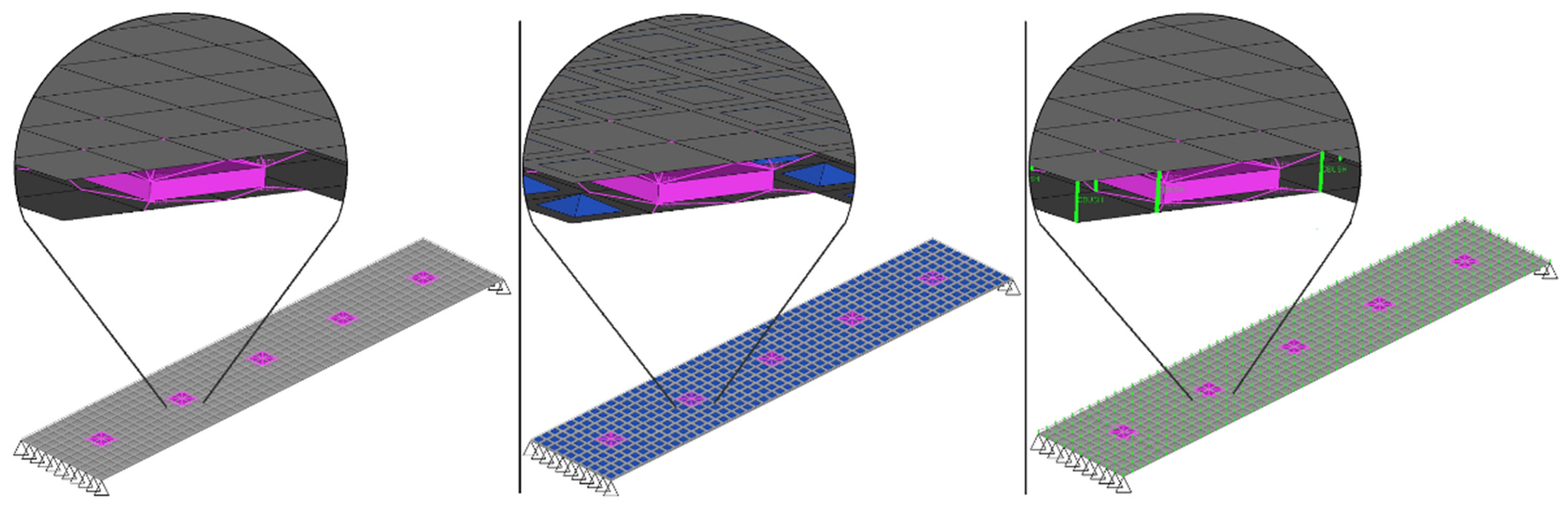
2.3. FE Test Models
2.3.1. Model Definition
- • Plate size [mm]: 250 × 50 × 1.0;
- • Gap between upper and lower plates: 1.0 mm;
- • Spot welds: 5 spots located every 50.0 mm; and
- • System support condition: simply supported.
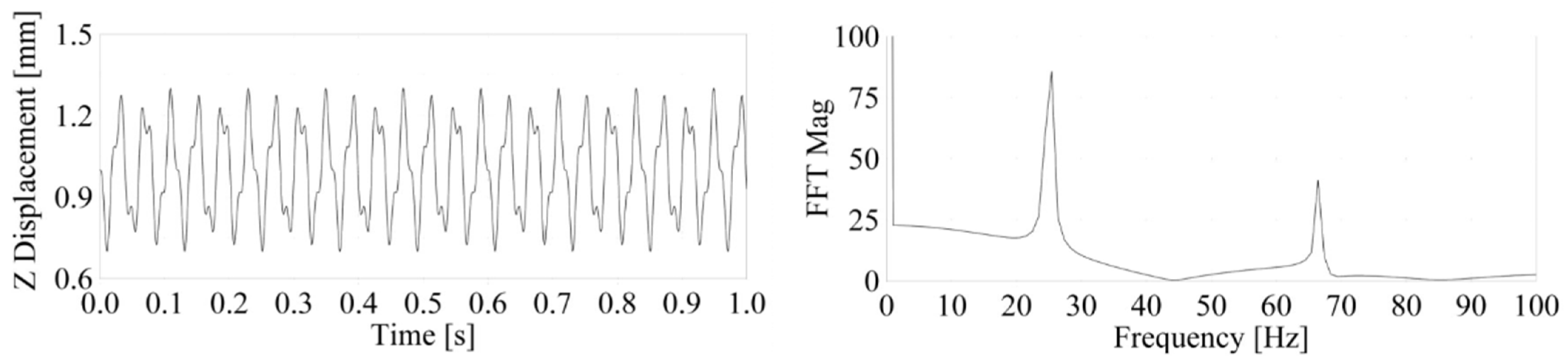
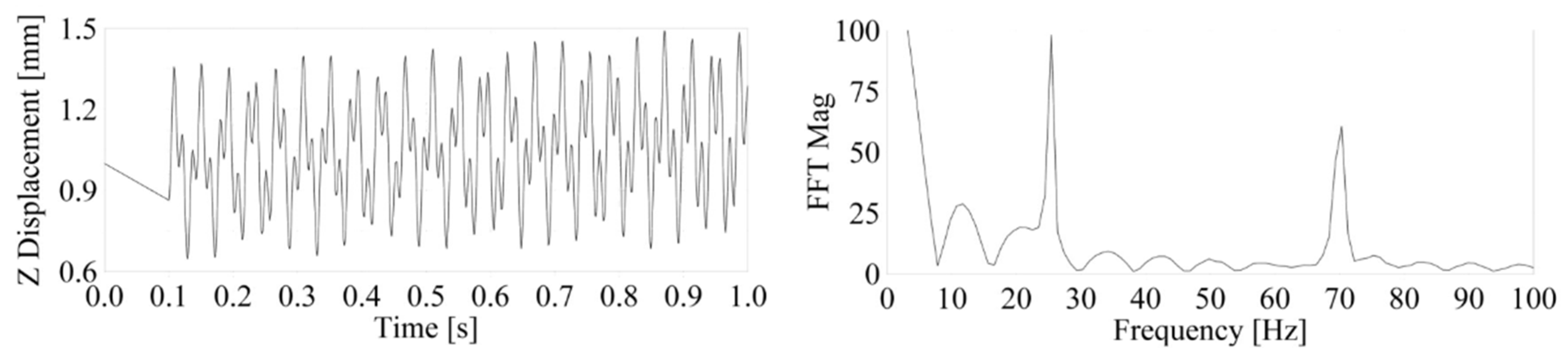
2.3.2. Comparison of the First Eigenfrequencies
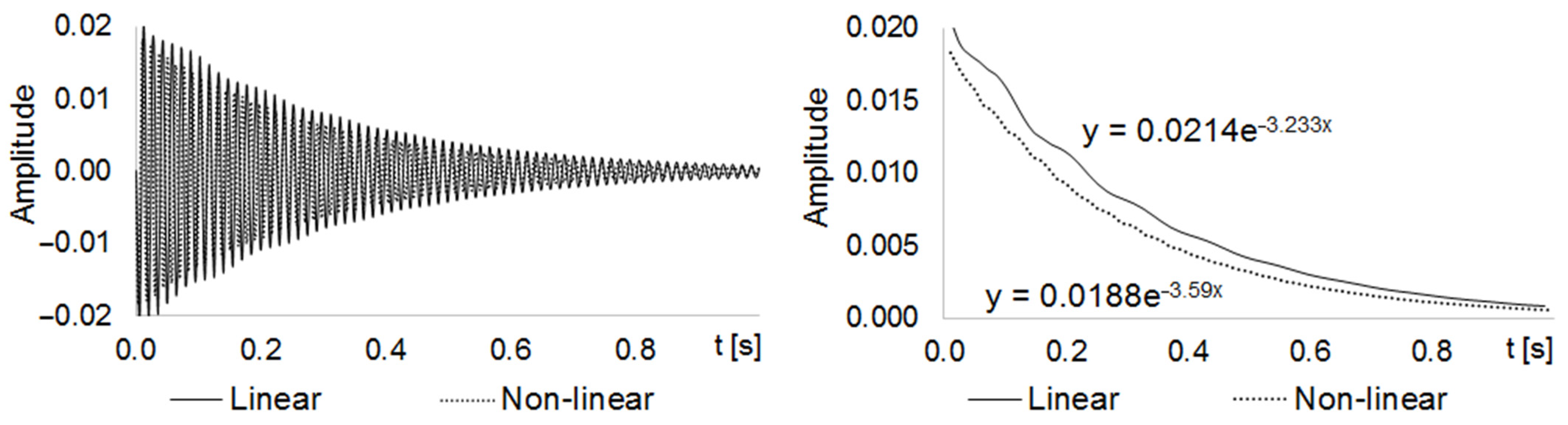
2.3.3. Comparison of the Damping Decay Curves
3. Results
3.1. Adjusted FE Model of the Vehicle Body Structure
3.1.1. Model Definition
3.1.2. Eigenfrequencies
3.1.3. MAC Matrices
3.1.4. FRAC Coefficients
3.1.5. Frequency Response Functions (FRFs)
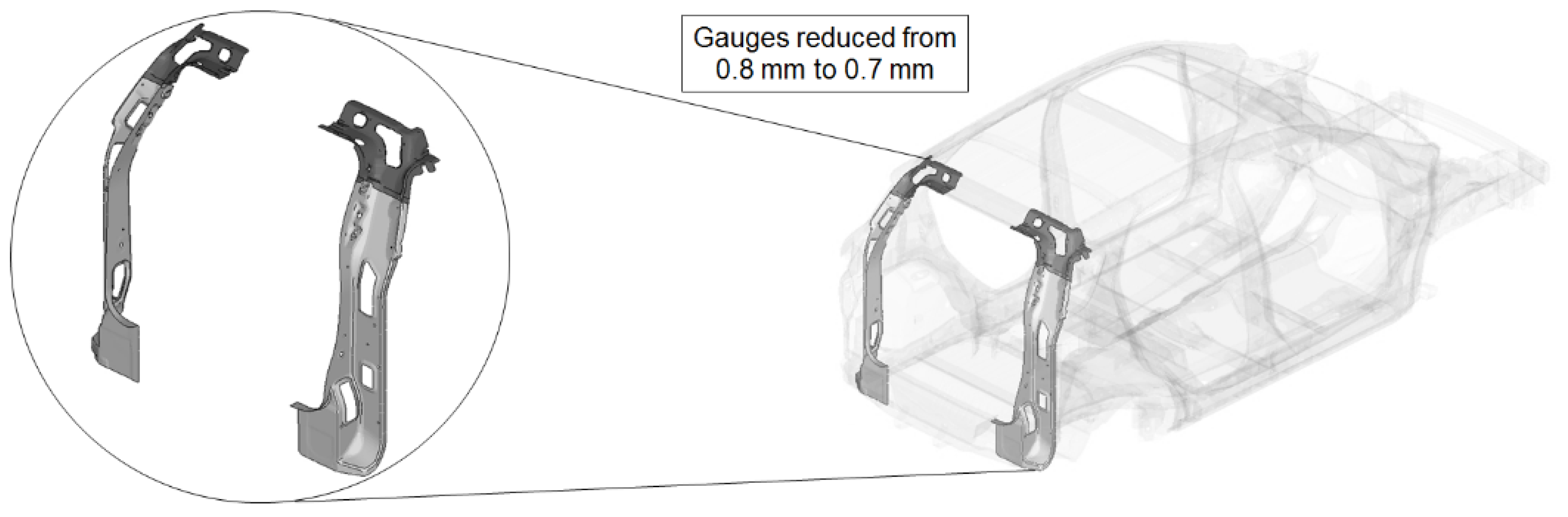
3.2. Optimization Analysis
- Disregard panels, since they were already set to the minimum gauge allowed;
- Disregard component brackets, since their main function is related to component tests;
- Avoid gauge changes smaller than 0.1 mm due to manufacturing restrictions;
- Avoid gauge changes higher than 15% of the initial gauge (if t < 1.0 mm) due to manufacturing restrictions for new tooling;
- Avoid gauge changes higher than 10% of the initial gauge (if t ≥ 1.0 mm) due to manufacturing restrictions for new tooling;
- Disregard critical parts related to frontal and lateral impact tests, since their main function is related to crash analysis; and
- Disregard critical parts related to chassis and powertrain attachments, since their main function is related to fatigue durability analysis.
- • Weight savings per vehicle: 0.566 kg
4. Discussion
- Both the reference and the adjusted models have a consistent correspondence with respect to the bench test data (MAC > 0.9). The adjusted model shows slightly better MAC correspondence than the reference model;
- The FRF curve of the adjusted model fits better with the bench test results than the FRF curve of the reference model, especially around the 33 and 39 Hz peaks; and
- The overall average FRAC coefficient of the adjusted model () showed an improvement of 9.1% compared to the overall average FRAC coefficient of the reference model ().
- Improve the accuracy of the mesh representation of welding spots by proposing new element formulations;
- Improve the accuracy of the mesh representation of bolted connections by proposing new element formulations;
- Improve the accuracy of the mesh representation of adhesive connection joints by proposing new element formulations;
- Refine the representation of the FE model by incorporating variations in sheet metal thickness from stamping manufacturing processes;
- Improve the accuracy of experimental bench test results by proposing new acquisition strategies for raw data measurements; and
- Improve the accuracy of experimental bench test results by proposing new data processing methods for both vibration and damping evaluation.
Author Contributions
Funding
Institutional Review Board Statement
Informed Consent Statement
Data Availability Statement
Acknowledgments
Conflicts of Interest
References
- Kraemer, J.C.; Bonnet, S. CAE methods in automotive industry: Overview of the stakes and prospects. In Proceedings of the 29th International Congress and Exhibition on Noise Control Engineering, Nice, France, 27–30 August 2000; pp. 27–30. [Google Scholar]
- Azadi, S.; Azadi, M.; Zahedi, F. NVH analysis and improvement of a vehicle body structure. J. Mech. Sci. Technol. 2009, 23, 2980–2989. [Google Scholar] [CrossRef]
- Center for Automotive Research. Automotive Product Development Cycles and the Need for Balance with the Regulatory Environment. 2017. Available online: www.cargroup.org/automotive-product-development-cycles-and-the-need-for-balance-with-the-regulatory-environment (accessed on 1 September 2019).
- Baker, M. Review of test/analysis correlation methods and criteria for validation of finite element models for dynamic analysis. In Proceedings of the 10th International Modal Analysis Conference, San Diego, CA, USA, 3–7 February 1992. [Google Scholar]
- Brughmans, M.; Leuridan, J.; Van Langenhove, T.; Turgay, F. Validation of Automotive Component FE Models by Means of Test-Analysis Correlation and Model Updating Techniques. SAE Tech. Paper 1999. [Google Scholar] [CrossRef]
- Schedlinski, C.; Wagner, F.; Bohnert, K.; Frappier, J.; Irrgang, A.; Lehmann, R.; Muller, A. Test-Based Computational Model Updating of a Car Body in White. Sound Vib. 2005, 39, 19–23. [Google Scholar]
- Splendi, L.; D’Agostino, L.; Baldini, A.; Castignani, L.; Pellicano, F.; Pinelli, M. Simplified Modeling Technique for Damping Materials on Light Structures: Experimental Analysis and Numerical Tuning. In Proceedings of the ASME International Mechanical Engineering Congress and Exposition, IMECE, San Diego, CA, USA, 15–21 November 2013. [Google Scholar]
- Rotondella, V.; Merulla, A.; Baldini, A.; Mantovani, S. Dynamic Modal Correlation of an Automotive Rear Sub-frame, with Particular Reference to the Modelling of Welded Joints. Adv. Acoust. Vib. 2017. [Google Scholar] [CrossRef] [Green Version]
- Peeters, P.; Manzato, S.; Tamarozzi, T.; Desmet, W. Reducing the impact of measurement errors in FRF-based substructure decoupling using a modal model. Mech. Syst. Signal Process. 2018, 99, 384–402. [Google Scholar] [CrossRef]
- Lim, J.H.; Hwang, D.S.; Sohn, D.; Kim, J.G. Improving the reliability of the frequency response function through semi-direct finite element model updating. Aerosp. Sci. Technol. 2016, 54, 59–71. [Google Scholar] [CrossRef]
- Arora, V.; Singh, S.P.; Kundra, T.K. Finite element model updating with damping identification. J. Sound Vib. 2009, 324, 1111–1123. [Google Scholar] [CrossRef]
- Lin, R.M.; Zhu, J. Model updating of damped structures using FRF data. Mech. Syst. Signal Process. 2006, 20, 2200–2218. [Google Scholar] [CrossRef]
- Marin, M.; Othman MI, A.; Seadawy, A.R.; Carstea, C. A domain of influence in the Moore–Gibson–Thompson theory of dipolar bodies. J. Taibah Univ. Sci. 2020, 14, 653–660. [Google Scholar] [CrossRef]
- Abbas, I.A.; Marin, M. Analytical Solutions of a Two-Dimensional Generalized Thermoelastic Diffusions Problem Due to Laser Pulse. Iran. J. Sci. Technol. Trans. Mech. Eng. 2018, 42, 57–71. [Google Scholar] [CrossRef]
- Bathe, K.J. Finite Element Procedures; Klaus-Jurgen Bathe: Watertown, NY, USA, 2014; pp. 887–978. [Google Scholar]
- Saeed, Z.; Firrone, C.; Berruti, T. Joint Identification through Hybrid Models Improved by Correlations. J. Sound Vib. 2021, 494, 115889. [Google Scholar] [CrossRef]
- Orban, F. Damping of materials and members in structures. In Proceedings of the 5th International Workshop on Multi-Rate Processes and Hysteresis (MURPHYS 2010), Pécs, Hungary, 31 May–3 June 2011; Volume 268, p. 012022. [Google Scholar]
- Mevada, H.; Patel, D. Experimental determination of structural damping of different materials. Proc. Eng. 2016, 144, 110–115. [Google Scholar] [CrossRef] [Green Version]
- Allemang, R.J. The modal assurance criterion—Twenty years of use and abuse. Sound Vib. 2003, 37, 14–23. [Google Scholar]
- Lee, D.; Ahn, T.S.; Kim, H.S. A metric on the similarity between two frequency response functions. J. Sound Vib. 2018, 436, 32–45. [Google Scholar] [CrossRef]
- Pastor, M.; Binda, M.; Harčarik, T. Modal assurance criterion. Proc. Eng. 2012, 48, 543–548. [Google Scholar] [CrossRef]
- Shin, K. An alternative approach to measure similarity between two deterministic transient signals. J. Sound Vib. 2016, 371, 434–445. [Google Scholar] [CrossRef]
- Haeussler, M.; Mueller, T.; Pasma, E.A.; Freund, J.; Westphal, O.; Voehringer, T. Component TPA: Benefit of including rotational degrees of freedom and over-determination. In Proceedings of the International Conference on Noise and Vibration Engineering, Leuven, Belgium, 7–9 September 2020; pp. 1135–1148. [Google Scholar]
- Ding, Q.; Chen, Y. Analyzing resonant response of a system with dry friction damper using an analytical method. J. Vib. Control 2008, 14, 1111–1123. [Google Scholar] [CrossRef]
- Lei, S.; Mao, K.; Li, L.; Xiao, W.; Li, B. Sensitivity analysis of a modal assurance criteria of damped systems. J. Vib. Control 2015, 23, 632–644. [Google Scholar] [CrossRef]
- Zhao, F.; Cao, S.Q.; Yu, Y.B.; Li, X.W. Theoretical study of the natural frequencies of a cantilever beam under dry friction. J. Vib. Control 2014, 22, 3779–3786. [Google Scholar] [CrossRef]
- Alciatore, D.; Histand, M. Introduction to Mechatronics and Measurement; McGraw Hill: New York, NY, USA, 2007; pp. 478–521. [Google Scholar]
- Lee, Y.L.; Barkey, M.; Kang, H.-T. Metal Fatigue Analysis Handbook: Practical Problem-Solving Techniques for Computer-Aided Engineering; Elsevier: Amsterdam, The Netherlands, 2012. [Google Scholar]
- Society of Automotive Engineers. SAE Ferrous Materials Standards Manual HS-30; Society of Automotive Engineers: Warrendale, PA, USA, 1999. [Google Scholar]
- Good Car Bad Car: Ford Ecosport Sales Figures. 2020. Available online: www.goodcarbadcar.net/ford-ecosport-sales-figures (accessed on 18 September 2021).
- Autoo: Best Selling Cars in Brazil in 2019. 2020. Available online: www.autoo.com.br/emplacamentos/veiculos-mais-vendidos/2019 (accessed on 18 September 2021).
- Car Salles Base: Ford Ecosport Europe Sales Figures. 2020. Available online: www.carsalesbase.com/europe-ford-ecosport/ (accessed on 18 September 2021).


| Mode | Frequency [Hz] | Damping c/co [ ] | Mode Shape | Mode Picture |
|---|---|---|---|---|
| 1 | 33.38 | 0.00513 | Windshield Torsion |  |
| 2 | 33.38 | 0.00390 | 1st Moonroof Bending | 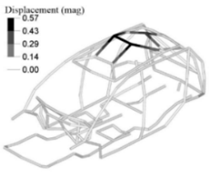 |
| 3 | 39.23 | 0.00567 | Global Torsion | 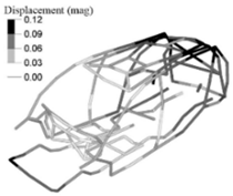 |
| 4 | 44.71 | 0.00228 | Global Lateral Bending | 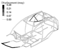 |
| 5 | 46.34 | 0.00642 | 2nd Moonroof Bending | 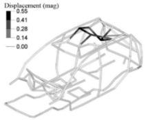 |
| 6 | 49.34 | 0.00344 | Moonroof Torsion |  |
| 7 | 53.73 | 0.00453 | Global Vertical Bending |  |
| - | - | BENCH TEST EIGENFREQUENCIES [Hz] | ||||||
|---|---|---|---|---|---|---|---|---|
| - | - | 33.4 | 33.4 | 39.2 | 44.7 | 46.3 | 49.3 | 53.7 |
| REFERENCE FE MODEL EIGENFREQUENCIES [Hz] | 31.3 | 0.97 | 0 | 0 | 0 | 0 | 0 | 0 |
| 36.2 | 0.02 | 0.98 | 0 | 0 | 0.07 | 0 | 0 | |
| 37.5 | 0 | 0.01 | 0.98 | 0 | 0 | 0 | 0 | |
| 43.2 | 0 | 0 | 0.01 | 0.96 | 0 | 0.01 | 0 | |
| 47.3 | 0.01 | 0 | 0 | 0.04 | 0.01 | 0.91 | 0 | |
| 50.2 | 0 | 0.09 | 0 | 0 | 0.95 | 0.02 | 0 | |
| 53.0 | 0 | 0 | 0 | 0 | 0.06 | 0 | 0.93 | |
| Impact Point/Dir | FRAC | Impact Point/Dir | FRAC | Impact Point/Dir | FRAC | |||
|---|---|---|---|---|---|---|---|---|
| REFERENCE FE MODEL RESPONSE POINT: X-DIR | front left/x | 0.9560 | REFERENCE FE MODEL RESPONSE POINT: Y-DIR | front left/x | 0.2315 | REFERENCE FE MODEL RESPONSE POINT: Z-DIR | front left/x | 0.8497 |
| front left/y | 0.2270 | front left/y | 0.1654 | front left/y | 0.1428 | |||
| front left/z | 0.4164 | front left/z | 0.2343 | front left/z | 0.6700 | |||
| front right/x | 0.9320 | front right/x | 0.1547 | front right/x | 0.5928 | |||
| front right/y | 0.1732 | front right/y | 0.1720 | front right/y | 0.1246 | |||
| front right/z | 0.3994 | front right/z | 0.2403 | front right/z | 0.4808 | |||
| rear left/x | 0.9647 | rear left/x | 0.2690 | rear left/x | 0.2206 | |||
| rear left/y | 0.8365 | rear left/y | 0.2645 | rear left/y | 0.4020 | |||
| rear left/z | 0.7581 | rear left/z | 0.1026 | rear left/z | 0.4220 | |||
| rear right/x | 0.9682 | rear right/x | 0.2488 | rear right/x | 0.3059 | |||
| rear right/y | 0.8887 | rear right/y | 0.2379 | rear right/y | 0.3238 | |||
| rear right/z | 0.6374 | rear right/z | 0.1110 | rear right/z | 0.5542 | |||
| Average x-dir | 0.6798 | Average y-dir | 0.2027 | Average z-dir | 0.4241 | |||
| - | - | - | - | - | - | Overall average | 0.4355 | |
| Mode | Modal Shape | Bench Test [Hz] | Reference FE Model [Hz] | Adjusted FE Model [Hz] |
|---|---|---|---|---|
| 1 | Windshield Torsion | 33.38 | 31.33 | 33.40 |
| 2 | 1st Moonroof Bending | 33.38 | 36.22 | 37.10 |
| 3 | Global Torsion | 39.23 | 37.52 | 40.01 |
| 4 | Global Lateral Bending | 44.71 | 43.19 | 44.87 |
| 5 | 2nd Moonroof Bending | 46.34 | 47.32 | 49.65 |
| 6 | Moonroof Torsion | 49.34 | 50.17 | 52.43 |
| 7 | Global Vertical Bending | 53.73 | 53.02 | 55.89 |
| - | - | BENCH TEST EIGENFREQUENCIES [Hz] | ||||||
|---|---|---|---|---|---|---|---|---|
| - | - | 33.4 | 33.4 | 39.2 | 44.7 | 46.3 | 49.3 | 53.7 |
| REFERENCE FE MODELEIGENFREQUENCIES [Hz] | 33.4 | 0.97 | 0 | 0 | 0 | 0 | 0 | 0 |
| 37.1 | 0.02 | 0.99 | 0 | 0 | 0.10 | 0 | 0 | |
| 40.0 | 0 | 0 | 0.99 | 0 | 0 | 0 | 0 | |
| 44.9 | 0 | 0 | 0 | 0.98 | 0 | 0 | 0 | |
| 49.7 | 0.01 | 0 | 0 | 0.03 | 0.01 | 0.93 | 0 | |
| 52.4 | 0 | 0.07 | 0 | 0 | 0.97 | 0.02 | 0 | |
| 55.9 | 0 | 0 | 0 | 0 | 0.02 | 0 | 0.96 | |
| Impact Point/Dir | FRAC | Impact Point/Dir | FRAC | Impact Point/Dir | FRAC | |||
|---|---|---|---|---|---|---|---|---|
| REFERENCE FE MODEL RESPONSE POINT: X-DIR | front left/x | 0.9666 | REFERENCE FE MODEL RESPONSE POINT: Y-DIR | front left/x | 0.1839 | REFERENCE FE MODEL RESPONSE POINT: Z-DIR | front left/x | 0.8323 |
| front left/y | 0.1859 | front left/y | 0.1795 | front left/y | 0.1909 | |||
| front left/z | 0.4848 | front left/z | 0.3990 | front left/z | 0.7250 | |||
| front right/x | 0.9846 | front right/x | 0.1181 | front right/x | 0.5154 | |||
| front right/y | 0.1774 | front right/y | 0.1946 | front right/y | 0.2316 | |||
| front right/z | 0.4986 | front right/z | 0.3854 | front right/z | 0.4522 | |||
| rear left/x | 0.9647 | rear left/x | 0.3333 | rear left/x | 0.2151 | |||
| rear left/y | 0.8627 | rear left/y | 0.3187 | rear left/y | 0.3266 | |||
| rear left/z | 0.8263 | rear left/z | 0.3838 | rear left/z | 0.3873 | |||
| rear right/x | 0.9657 | rear right/x | 0.2916 | rear right/x | 0.3961 | |||
| rear right/y | 0.9432 | rear right/y | 0.3388 | rear right/y | 0.2362 | |||
| rear right/z | 0.6384 | rear right/z | 0.3813 | rear right/z | 0.5864 | |||
| Average x-dir | 0.7082 | Average y-dir | 0.2923 | Average z-dir | 0.4246 | |||
| - | - | - | - | - | - | Overall average | 0.4751 | |
Publisher’s Note: MDPI stays neutral with regard to jurisdictional claims in published maps and institutional affiliations. |
© 2021 by the authors. Licensee MDPI, Basel, Switzerland. This article is an open access article distributed under the terms and conditions of the Creative Commons Attribution (CC BY) license (https://creativecommons.org/licenses/by/4.0/).
Share and Cite
Martins, L.; Romero, G.; Suarez, B. Enhancing the Accuracy of Linear Finite Element Models of Vehicle Structures Considering Spot-Welded Flanges. Materials 2021, 14, 6075. https://doi.org/10.3390/ma14206075
Martins L, Romero G, Suarez B. Enhancing the Accuracy of Linear Finite Element Models of Vehicle Structures Considering Spot-Welded Flanges. Materials. 2021; 14(20):6075. https://doi.org/10.3390/ma14206075
Chicago/Turabian StyleMartins, Luis, Gregorio Romero, and Berta Suarez. 2021. "Enhancing the Accuracy of Linear Finite Element Models of Vehicle Structures Considering Spot-Welded Flanges" Materials 14, no. 20: 6075. https://doi.org/10.3390/ma14206075