Abstract
The failures of soil slopes during the construction of high-speed railway caused by the soil after the freeze–thaw (F–T) cycle and the subsequent threat to construction safety are critical issues. An appropriate constitutive model for soils accurately describing the deformation characteristics of soil slopes after the F–T cycle is very important. Few constitutive models of soils incorporate the F–T cycle, and the associated flow rule has always been employed in previous models, which results in an overestimation of the deformation of soil exposed to the F–T cycle. Generalized plasticity theory is widely used to predict the performance of geotechnical materials and is especially well adapted to deal with this type of generalized cyclic loading (such as a freeze–thaw cycle), and it overcomes the shortcomings of the associated flow rule that causes larger shear deformation. To this end, an elastoplastic model framework based on generalized plasticity theory with double yield surfaces for saturated soils subjected to F–T cycles was developed. Two types of plastic deformation mechanisms, i.e., plastic volumetric compression and plastic shear, were considered in this elastoplastic model. It was found that this model can accurately predict the mechanical behavior and deformation characteristics of saturated soils after F–T cycles.
1. Introduction
High-speed railways in China have developed rapidly over the last decade [1]. By the end of 2021, the total length of the high-speed railway systems in China is expected to be more than 40,000 km. A high-speed railway has been constructed in a typical seasonally frozen region of Northeast China [2,3]. The freeze–thaw (F–T) cycle is one of the most common physical weathering processes in these regions [4] and significantly affects the mechanical behavior of soils [5,6,7,8,9,10,11,12,13]. Some studies have reported that F–T cycles induce cutting slope failures (Figure 1) [14] during the construction of high-speed railway. An appropriate constitutive model for soils that accurately describes the deformation characteristics of soil slope after the F–T cycle is very important.
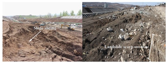
Figure 1.
The cutting slope failures along the high-speed railway (the left figure is from [14]).
Recently, many studies have been carried out to analyze the effect of wet/dry cycles on the deformation behavior and constitutive stress–strain of soil [15,16,17,18,19]. Furthermore, a number of researchers, such as Li et al. 2019 [20], Li and Yang, 2018 [21], Guo et al. 2021 [22], and Li et al. 2020 [23], have studied the elastoplastic model of unsaturated soils, incorporating different influencing factors. However, the literature about the constitutive model of saturated soils considering the effect of the F–T cycle is relatively sparse. Furthermore, the associated flow rule was usually adopted in the constitutive model of soils [24,25]. The traditional associated flow rule always induces larger shear deformation [26,27], which overestimates the deformation of soil slopes exposed to the F–T cycle.
Generalized plasticity theory is widely used to predict the performances of geotechnical materials [28,29]. The effect of freezing–thawing cycles on the behavior of soils is a matter of great practical importance. Generalized plasticity is especially well adapted to deal with this type of generalized cyclic loading [29]. The generalized plasticity theory does not obey the traditional assumption of plastic potential function, nor does it comply with the associated plastic flow rule [28]. It overcomes the shortcomings of the associated flow rule causing larger shear deformation. As a result, the use of the framework of generalized plasticity theory is particularly useful to evaluate the mechanical behavior of soil. However, few models for soils subjected to the F–T cycle have been based on the generalized plasticity theory.
In this study, an elastoplastic model for saturated soils subjected to F–T cycles under the framework of generalized plasticity theory with double yield surfaces was developed. The derivation of the model and the estimation of the model parameters are presented in detail. The triaxial test results of the saturated soils were predicted by the proposed model, and finally, the effectiveness of the model was verified using the test data.
2. An Elastoplastic Model Framework for Saturated Soils in Generalized Plasticity Theory Incorporating the Effects of the Freeze–Thaw Cycle
An elastoplastic model framework for saturated soils subjected to F–T cycles was developed using the generalized plasticity theory. Moreover, a detailed introduction to the generalized plasticity theory is presented in the Appendix A.
2.1. Elastic Deformations
In this section, the elastic deformations are discussed, and the soil is regarded as isotropic and elastic within the yield surface. The increments in the strain invariants consist of two parts [30], i.e.,
where dεs, d, and d are the increment of shear strain, elastic shear strain, and plastic shear strain, respectively; and dεv, d, and d are the increment of volumetric strain, elastic volumetric strain, and plastic volumetric strain, respectively.
The elastic components of the strain increments (d and d) can be obtained from
where p′ and q are the mean effective stress and deviator stress, respectively; p′ = (σ′1 +σ′2 + σ′3), q = σ′1 − σ′3. σ′1, σ′2, and σ′3 are the major principal effective stress, the intermediate principal effective stress, and the minor principal effective stress, respectively. G and K are the shear modulus and bulk modulus, respectively, and can be deduced from the elastic modulus (E) for an assumed value of Poisson’s ratio (v):
2.2. Yield Surfaces and Plastic Potential Functions
The deformation of soil slope after the F–T cycle, which includes the shear deformation, compression deformation, or a combination of the two deformations, is complicated. The double yield surfaces proposed by Yin (1988) [31] could reflect two types of plastic deformation mechanisms, namely, plastic volumetric compression and plastic shear for soils, and it is often employed by researchers [24,32] to present the mechanical and deformation characteristics of soils. Therefore, the double yield surfaces proposed by Yin (1988) [19] were used in this paper.
Figure 2a shows the two yield surfaces proposed by Yin (1988) [31] in the q-p′ plane. Point A is the intersection of the two yield surfaces. Referring to the yield surfaces in [31], the yield surfaces of soils subjected to F–T cycling are plotted in Figure 2b. Two yield surfaces divide the q-p′ plane into four parts [31]: region Z0 only has elastic deformation, region Z1 is only related to the first yield surface, region Z2 is only related to the second yield surface, and the two kinds of plastic deformation exist simultaneously in region Z3.
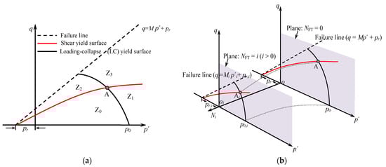
Figure 2.
Yield surfaces in q-p′ space: (a) Yin’s proposed yield surfaces (1988); (b) yield surfaces under freeze–thaw cycles.
In the first yield surface (fv), the loading–collapse (LC) yield surface represents the compression mechanism and is expressed as the following form:
where M1, p0, and pr are the LC yield surface indexes that are related to the shape of the stress–strain curve of soils, the initial mean effective stress, and the intercept of the failure line on the p′ axis, respectively.
In addition, symbols Mi, p′i, pr,i, and p0,i are the parameters under various numbers of freeze–thaw cycles (NFT), which are the slope of failure line, mean effective stress, intercept of the failure line on the p′ axis, and initial mean effective stress, respectively. Subscript i represents the number of freeze–thaw cycles (i = 0, 1, 3, 7, and 11), which is the same meaning as NFT. For convenience, the symbol i was used in this section.
A hyperbolic curve is used to predict the relation between plastic volumetric strain () and p0 [31]:
The was chosen as the hardening parameter. A non-associated plastic flow rule was adopted in this model. Referring to [33], the mean effective stress p′ is assumed to be the plastic potential function (Qv) corresponding to the plastic volumetric strain.
Qv = p′
The second yield surface (fq) proposed by Yin (1988) [31] is employed to present the shearing mechanism of the soils:
where a and M2 are the elastoplastic dilation index and shear yield surface index that is related to the slope of failure line (M), respectively. is the plastic shear strain.
Similarly, is used as the hardening parameter for the second yield surface. Referring to [33], the plastic potential function (Qq) is assumed to be q, corresponding to the plastic shear strain.
Qq = q
2.3. Elastoplastic Stress–Strain Relations
The incremental stress–strain relationship of soils in p′ − q plane can be obtained [28]:
where dλv and dλq are the plastic factors (see Appendix A). The elastic stiffness matrix, [De], can be determined by Equation (13):
Based on Equations (9), (11), (12), (A12), and (A13), the following expressions can be obtained [28]:
where Av and Aq are the plastic parameters.
The related parameters are given by
The elastoplastic incremental stress–strain relationship can be given by
According to [28], the elastoplastic stiffness matrix [Dep] takes the following form:
where w1 and w2 are given by
where t1, t2, t3, t4, t5, and t6 can be obtained by Equations (A16)–(A21) (see Appendix A).
3. Determination of Parameters and Model Validation
The parameters employed in the model fall into three categories: elastic parameters, parameters related to the compressive mechanism, and parameters related to the shear mechanism. The model was employed to predict the test data for soils after the F–T cycle.
3.1. Elastic Parameters
The elastic parameters (G and K) can be determined from triaxial compressive loading–unloading–reloading testing. Moreover, G and K can also be obtained from Equations (5) and (6), whereas the value of Poisson’s ratio (v) equal to 0.3 is assumed in this model [34,35].
3.2. Parameters Related to a Compressive Mechanism
The LC yield surface index, M1, which is related to the shape of stress–strain curve, is calculated through the following equation [31]:
where β is the ratio of the volumetric strain (εv) to axial strain (εa) when the stress level equals 75%; the mean value was used in the model under different confining pressure (σc) and various NFT values. M is the slope of the failure line, and it is also related to NFT.
M1 = (1 + 0.25β2)M
The value of pr can be obtained from the failure line under various NFT values. The elastoplastic compression indexes (χ1 and χ2) have been reported by Yin (1988) [31] and will not be repeated here. However, a material parameter Γ was added in the equation (see Yin 1988 [31]) to represent the material characteristics (it is related to volumetric compression deformation, = 2.5–3.0).
3.3. Parameters Related to a Shear Mechanism
The shear yield surface index, M2, which is related to the shape of the q-deviatoric strain (εs) curve, can be estimated by the following equation [31]:
where Rf is the failure ratio, which is defined by
where qf and qult are the failure strength and the asymptotic value of deviatoric stress for the q − εs curve, respectively.
Rf = qf / qult
The elastoplastic dilation index (a) reflects the proportion of the strain induced by the shear yield surface in terms of the total strain. It can be estimated by the equation proposed by Yin (1988) (a = 0.25 − 0.15d, d is the slope of the εv − εa curve at a stress level between 75% and 95%).
In summary, two elastic parameters (G and K), four parameters (M1, pr, χ1, and χ2) related to the compressive mechanism, and two parameters (M2 and a) related to the shear mechanism were used in the proposed model. These eight parameters change along NFT and they are all functions of NFT. These parameters can be obtained by test results under different NFT values and empirical formulas.
3.4. Model Validation
The influence of the F–T cycle on the mechanical properties of silty clay was investigated by Cui et al. (2015) [36]. The triaxial test results of saturated silty clay exposed to three and five F–T cycles were used to verify the correctness of the model. The volumetric strain was measured under consolidation and shearing in [36]. The volumetric strain induced by consolidation was not given, so the volumetric strain during shearing could not be obtained. Therefore, only the stress–strain curves of the saturated silty clay were employed to verify the model’s correctness. The model parameters used in [36] for the third and fifth F–T cycle are shown in Table 1 and Table 2. Figure 3 plots the comparison between the experimental data and predicted results. From Figure 3, considering some parameter determination based on the empirical formula, the predicted values are within reasonable range, although there are some differences. In addition, the triaxial test results of bioenzyme-treated saturated soils with 3% bioenzyme from Wen and Wang (2018) [37] were also used to verify the model’s correctness. (although the bioenzyme-treated saturated soils are not subjected to the F–T cycle, the validation results can be used as proof that the model framework can be widely used). Model parameters used in [37] are given in Table 3. Form Figure 4, the stress–strain curve and volumetric–deviatoric strain curve of bioenzyme-treated saturated soils were reasonably predicted by the proposed model.

Table 1.
Parameter values for the proposed elastoplastic model with NFT = 3 used in [36].
Table 2.
Parameter values for the proposed elastoplastic model with NFT = 5 used in [36].
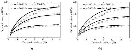
Figure 3.
Comparison between predicted and observed results for stress–strain curves of saturated silty clay (data from [36]): (a) NFT = 3 and (b) NFT = 5.
Table 3.
Parameter values for the proposed elastoplastic model used in [37].
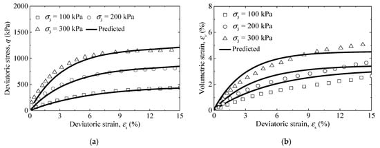
Figure 4.
Comparison between predicted and observed results: (a) stress–strain curve, and (b) volumetric–deviatoric strain curve of bioenzyme-treated saturated soils (data from [37]).
4. Future Fields of Application
This study presents an elastoplastic model framework for saturated soils subjected to the freeze–thaw cycle and also serves as a simple methodology to establish the constitutive model for soils. Two types of plastic deformation mechanisms, i.e., plastic volumetric compression and plastic shear, were considered in this elastoplastic model. Therefore, this model could be employed to analyze the relatively complex deformations of engineering, such as soil slope, railway roadbed, dam, and building foundation. In addition, the analysis discussed in this paper is mainly used to describe the deformation characteristics of strain hardening for clay soils. In practical applications, this important aspect must be given proper attention. Further study is needed for a more quantitative description of the strain softening of soils.
5. Conclusions
In this study, an elastoplastic model framework for saturated soils subjected to the freeze–thaw cycle based on the generalized plasticity theory was proposed. The primary conclusions from this work can be given as follows:
(1) This model was on the framework of the generalized plasticity theory overcoming the disadvantage of the traditionally associated flow rule, inducing larger shear deformation. The model adequately describes the contractive shear behavior of saturated soils under different freeze–thaw cycles.
(2) The capabilities of this model are illustrated by predicting the triaxial tests of silty clay and bioenzyme-treated soils. In this model, the overall elastoplastic model behaviors of saturated soils are described through eight model parameters that are specifically associated with the freeze–thaw cycle.
Further work will focus on the derivation of the elastoplastic constitutive model of soil after the freeze–thaw cycle in a real triaxial stress state and consider unsaturated conditions and more general stress paths.
Author Contributions
Conceptualization and methodology, S.C.; validation, X.L. (Xianzhang Ling); writing—original draft preparation, S.C.; writing—review and editing, X.L. (Xinyu Li) and L.G.; visualization, W.X. and G.L. All authors have read and agreed to the published version of the manuscript.
Funding
This research was supported by the National Key R&D Program of China (Grant No. 2018YFC1505305), the National Major Scientific Instruments Development Project of China (Grant No. 41627801), the National Natural Science Foundation of China (Grant Nos. 42101125 and 41772315), the Open Research Fund Program of State Key Laboratory of Frozen Soil Engineering of China (Grant No. SKLFSE202015), China Postdoctoral Science Foundation Project (2021M690840), and the Technology Research and Development Plan Program of Heilongjiang Province (Grant No. GA19A501).
Institutional Review Board Statement
Not applicable.
Informed Consent Statement
Not applicable.
Data Availability Statement
Not applicable.
Acknowledgments
The authors wish to thank the editor and the reviewers for their contributions to the paper.
Conflicts of Interest
The authors declare no conflict of interest.
Appendix A. Theoretical Framework of Generalized Plasticity Theory
Generalized plasticity theory is widely used to analyze the behavior of geotechnical materials [28]. According to the theory of plasticity, the strain increment (dεij) is usually divided into an elastic component (d) and a plastic component (d) [28]:
The generalized potential theory can be expressed in the following form [28,33]:
where Qk is the plastic potential function. Q1, Q2, and Q3 should be non-associated. dλk and σij are the plastic factors corresponding to the plastic potential function and stress increments, respectively.
The yield surfaces should be coincident with the plastic potential surface [28]. The volumetric yield function fv (p′, q, θσ, hv), the shear yield function fq (p′, q, θσ, hq) in the q-direction, and the shear yield function fθ (p′, q, θσ, hθ) in the θσ-direction take the following form [28]:
Differentiating Equations (A3)–(A5) and combining Equation (A2) gives [28]
The plastic parameters, Av, Aq, and Aθ can be given by [28,33]
where hv, hq, and hθ are the hardening parameters.
The effect of θσ is very small and can be ignored [28,33]. Hence, Equations (A6)–(A8) can be rewritten as
The plastic factors dλv and dλq are computed as follows [28]:
where t1, t2, t3, t4, t5, and t6 can be expressed as [28]
References
- Tang, L.; Kong, X.; Li, S.; Ling, X.; Ye, Y.; Tian, S. A preliminary investigation of vibration mitigation technique for the high-speed railway in seasonally frozen regions. Soil Dyn. Earthq. Eng. 2019, 127, 105841. [Google Scholar] [CrossRef]
- Liu, J.; Wang, T.; Tian, Y. Experimental study of the dynamic properties of cement- and lime-modified clay soils subjected to freeze–thaw cycles. Cold Reg. Sci. Technol. 2010, 61, 29–33. [Google Scholar] [CrossRef]
- Zhang, S.; Sheng, D.; Zhao, G.; Niu, F.; He, Z. Analysis of frost heave mechanisms in a high-speed railway embankment. Can. Geotech. J. 2016, 53, 520–529. [Google Scholar] [CrossRef]
- Hu, T.; Liu, D.W.; Wu, H. Experimental testing and numerical modelling of mechanical behaviors of silty clay under freez-ing-thawing cycles. Math. Probl. Eng. 2020, 2020, 1–13. [Google Scholar]
- Aubert, J.; Gasc-Barbier, M. Hardening of clayey soil blocks during freezing and thawing cycles. Appl. Clay Sci. 2012, 65–66, 1–5. [Google Scholar] [CrossRef]
- Al-Omari, A.; Beck, K.; Brunetaud, X.; Ákos, T.; Al-Mukhtar, M. Critical degree of saturation: A control factor of freeze-thaw damage of porous limestones at Castle of Chambord, France. Eng. Geol. 2015, 185, 71–80. [Google Scholar] [CrossRef]
- Mardani-Aghabaglou, A.; Kalıpcılar, I.; Sezer, G.I.; Sezer, A.; Altun, S. Freeze-thaw resistance and chloride-ion penetration of cement-stabilized clay exposed to sulfate attack. Appl. Clay Sci. 2015, 115, 179–188. [Google Scholar] [CrossRef]
- Liu, J.; Chang, D.; Yu, Q. Influence of freeze-thaw cycles on mechanical properties of a silty sand. Eng. Geol. 2016, 210, 23–32. [Google Scholar] [CrossRef]
- Lu, Y.; Liu, S.; Weng, L.; Wang, L.; Li, Z.; Xu, L. Fractal analysis of cracking in a clayey soil under freeze–thaw cycles. Eng. Geol. 2016, 208, 93–99. [Google Scholar] [CrossRef]
- Consoli, N.C.; Da Silva, K.; Filho, S.; Rivoire, A.B. Compacted clay-industrial wastes blends: Long term performance under extreme freeze-thaw and wet-dry conditions. Appl. Clay Sci. 2017, 146, 404–410. [Google Scholar] [CrossRef]
- Tang, L.; Cong, S.; Ling, X.; Xing, W.; Nie, Z. A unified formulation of stress-strain relations considering micro-damage for expansive soils exposed to freeze-thaw cycles. Cold Reg. Sci. Technol. 2018, 153, 164–171. [Google Scholar] [CrossRef]
- Xu, J.; Li, Y.; Lan, W.; Wang, S. Shear strength and damage mechanism of saline intact loess after freeze-thaw cycling. Cold Reg. Sci. Technol. 2019, 164, 102779. [Google Scholar] [CrossRef]
- Liu, J.J.; Zha, F.S.; Xu, L.; Kang, B.; Yang, C.B.; Zhang, W.; Zhang, J.W.; Liu, Z.H. Zinc leachability in contaminated soil stabi-lized/solidified by cement-soda residue under freeze-thaw cycles. Appl. Clay Sci. 2020, 186, 105474. [Google Scholar] [CrossRef]
- Xiang, D. Study on the Failure Mechanism and Control Technology of Deep Cutting Slope Located on High-Cold Area. Master Thesis, Southwest Jiaotong University, Chengdu, China, 2017. [Google Scholar]
- Diel, J.; Vogel, H.-J.; Schlüter, S. Impact of wetting and drying cycles on soil structure dynamics. Geoderma 2019, 345, 63–71. [Google Scholar] [CrossRef]
- Zhao, N.F.; Ye, W.M.; Chen, B.; Chen, Y.G.; Cui, Y.J. Modeling of the swelling–shrinkage behavior of expansive clays during wetting–drying cycles. Acta Geotech. 2018, 14, 1325–1335. [Google Scholar] [CrossRef]
- Evolution of fissures and bivariate-bimodal soil-water characteristic curves of expansive soil under drying-wetting cycles. Chin. J. Geotech. Eng. 2021, 43, 58–63.
- Li, W.; Zeng, S.; Zhao, J.; Liu, P. Damage characteristics of Changsha ring expressway silty clay during dry-wet cycle. J. Cent. South Univ. 2017, 48, 1360–1366. [Google Scholar]
- Hao, Y.Z.; Wang, T.H.; Cheng, L.; Jin, X. Structural constitutive relation of compacted loess considering the effect of drying and wetting cycles. Rock Soil Mech. 2021, 42, 1–10. [Google Scholar]
- Li, J.; Yin, Z.Y.; Cui, Y.J.; Liu, K.; Yin, J.H. An elasto-plastic model of unsaturated soil with an explicit degree of satura-tion-dependent CSL. Eng. Geol. 2019, 260, 105240. [Google Scholar] [CrossRef]
- Li, W.; Yang, Q. Hydromechanical Constitutive Model for Unsaturated Soils with Different Overconsolidation Ratios. Int. J. Géoméch. 2018, 18, 04017142. [Google Scholar] [CrossRef]
- Guo, N.; Chen, Z.H.; Yang, X.H.; Guo, J.F. Incremental nonlinear constitutive model and parameter variation of transversely isotropic unsaturated soil. Chin. J. Geotech. Eng. 2021. [Google Scholar]
- Li, X.X.; Li, T.; Peng, L.Y. Elastoplastic two-surface model for unsaturated cohesive soils under cyclic loading with controlled matric suction. Rock Soil Mech. 2020, 41, 552–560. [Google Scholar]
- Hu, T.F.; Liu, J.K.; Wang, T.L.; Yue, Z.R. Effect of freeze-thaw cycles on the deformation characteristics of a silty clay and its constitutive model with double yielding surfaces. Rock Soil Mech. 2018, 40, 1–11. [Google Scholar]
- Zhang, X.D.; Ren, K.; Zhang, H.D.; Xing, Y.D.; Yang, J.J. Constitutive relationship with double yield surfaces for cinder im-proved soil under freeze-thaw cycles. Chin. J. Rock Mech. Eng. 2018, 37, 1916–1923. [Google Scholar]
- Kong, L.; Zheng, Y.R.; Wang, Y.C. A three-yield surface model for soilmasses based on the generalized plastic mechanics. Rock Soil Mech. 2000, 21, 108–112. [Google Scholar]
- Zheng, Y.R. New development of geotechnical plastic mechanics-generalized plastic mechanics. Chin. J. Geotech. Eng. 2003, 25, 1–10. [Google Scholar]
- Lai, Y.M.; Yang, Y.G.; Chang, X.X.; Li, S.Y. Strength criterion and elastoplastic constitutive model of frozen silt in generalized plastic mechanics. Int. J. Plasticity 2010, 26, 1461–1484. [Google Scholar]
- Sa´nchez, M.; Gens, A.; Guimaraes, L.J.; Olivella, S. A double structure generalized plasticity model for expansive materials. Int. J. Numer. Anal. Met. Geomech. 2005, 29, 751–787. [Google Scholar] [CrossRef]
- Salim, W.; Indraratna, B. A new elastoplastic constitutive model for coarse granular aggregates incorporating particle break-age. Can. Geotech. J. 2004, 41, 657–671. [Google Scholar] [CrossRef]
- Yin, Z.Z. Stress-strain model of soils with double-yield surfaces. Chin. J. Geotech. Eng. 1988, 10, 64–71. [Google Scholar]
- Lu, Z.H.; Chen, Z.H. An elastoplastic damage constitutive model of unsaturated undisturbed expansive soil. Chin. J. Geotech. Eng. 2003, 25, 422–426. [Google Scholar]
- Cai, X.; Yang, J.; Guo, X.W.; Wu, Y.L. Elastoplastic constitutive model for cement-sand-gravel material. Chin. J. Geotech. Eng. 2016, 380, 1569–1577. [Google Scholar]
- Alonso, E.; Vaunat, J.; Gens, A. Modelling the mechanical behaviour of expansive clays. Eng. Geol. 1999, 54, 173–183. [Google Scholar] [CrossRef] [Green Version]
- Yao, Y.; Zhou, A. Non-isothermal unified hardening model: A thermo-elasto-plastic model for clays. Géotechnique 2013, 63, 1328–1345. [Google Scholar] [CrossRef]
- Cui, H.H.; Liu, J.K.; Zhang, L.Q.; Tian, Y.H. A constitutive model of subgrade in a seasonally frozen area with considering freeze-thaw cycles. Rock Soil Mech. 2015, 36, 2228–2236. [Google Scholar]
- Wen, C.P.; Wang, J.J. Study on the stress-strain characteristics of bioenzyme-treated expansive soil based on Shen Zhujiang′s double yield surfaces elasto-plastic model. Chin. J. Rock Mech. Eng. 2018, 37, 1011–1019. [Google Scholar]
Publisher’s Note: MDPI stays neutral with regard to jurisdictional claims in published maps and institutional affiliations. |
© 2021 by the authors. Licensee MDPI, Basel, Switzerland. This article is an open access article distributed under the terms and conditions of the Creative Commons Attribution (CC BY) license (https://creativecommons.org/licenses/by/4.0/).