Abstract
Various methods are available for the calculation of timber–concrete composite floors. The gamma method, which is important in construction practice, as well as the differential equation method, are based on the simplified assumption of a continuous bond between wood and concrete. This makes it possible to analytically calculate the internally statically indeterminate partial section sizes and deformation sizes, analogous to the force size method. In this paper, two typical load situations of concentrated loads (central and off-centre) were analytically and numerically evaluated and compared using the above-mentioned methods (gamma and differential equation), with a discrete method for the case of a timber beam reinforced with a concrete slab using screws as fasteners. The calculation results show significant deviations, which speak for the application of discrete methods in certain load situations and thus limit the usability of the gamma method under certain conditions. For the problem of deflection determination, which is not dealt with in the literature for the discrete method, a numerical method is described in the present work, which was first developed and presented by the first author.
1. Introduction
Wood is becoming increasingly important in multi-story residential and office construction as a natural and sustainable building material. In addition to the ecological advantages, the favourable indoor climate and natural appearance of wood surfaces on walls and ceilings are also in the foreground. Here, the wood–concrete composite construction method, which makes optimum use of the mechanical properties of both building materials, has proved to be particularly forward-looking. A large part of the applications of this method is carried out as reinforcement systems for existing wooden ceilings, especially in connection with the overall building stiffness under earthquake loads. For sustainability reasons, wood–concrete composite floors are also increasingly being used in new buildings, especially with the use of CLT (cross-laminated timber) panels.
The lower wooden element, in the form of beams or slabs, mainly carries the bending tensile forces, while the upper continuous concrete slab mainly carries the bending compressive forces. The necessary shear connection is made with various elements, such as bolts, screws, shear collars (cleats), etc. These form a compliant, or elastic, bond between the two elements, which leads to a load-bearing behaviour that lies between no- (loose) and rigid-bond behaviour.
The following is a brief summary of the development of wood–concrete composite floors based on the literature. The first wood–concrete composite floors were developed about 100 years ago, as indicated by Holschemacher et al. in [1], Yeoh et al. in [2] and Grosse et al. in [3]. Design formulas were developed or adopted from Kolbitsch et al. [4] and modified from the “doweled beam theory”. A comparison of the calculation methods was made by Grosse et al. in [5]. The long-term behaviour was modified by Kuhlmann et al. [6] using the gamma method. It was also treated by Grosse et al. [7], Avak et al. [8] and Gerold et al. [9]. Schmidt et al. compared the gamma method with the finite element method in [10] and gave design proposals with graded fastener spacing in [11]. In [12], Rautenstrauch et al. showed a practical design using the framework model. The behaviour of CLT–concrete composite floors with the extended gamma method and the finite element method was investigated by Forsberg et al. in [13], based on the work of Wallner et al. [14].
Essential for load-bearing behaviour are the connecting elements between the wood and concrete. In [15], fully threaded screws were investigated by Heller, and in [16], dowel bars were discussed by Schröter et al. Bonded connections were treated by Schäfers et al. in [17]. Numerical modelling was performed for cleats by Grosse et al. [18], and appropriate models and failure criteria were applied by Schönborn et al., who gave design rules for shear collars in [19]. In one of the newest papers [20], Woschitz et al. described bending tests with CLT and prefabricated concrete plates and compared the calculation methods. In [21], the state-of-the-art of timber–concrete composite structures from cost (European Cooperation in Science and Technology) is described. This documentation forms the basis for the new Eurocode.
For the simplified calculation of wood–concrete composite floors, the strictly spatial system is reduced to an elastically coupled flexural beam system, for which several calculation methods are now available. The differences between the methods result, on the one hand, from the different methods used to generate the static model, and on the other hand, from system-specific conditions (in particular the types of action) that lead to different governing equations.
In this paper, the gamma method according to Möhler [22] and Heimeshoff [23], which is established in practice and relatively easy to calculate, and which is prescribed by Eurocode 5 [24], is compared to and evaluated with the more stringent differential equation method according to Natter and Hoeft [25], as well as the discrete method according to Stüssi [26,27] and Huber [28], on the basis of a representative design situation for selected load cases. This is especially relevant, since the gamma method is known to provide exact, or satisfactorily accurate, results only for symmetrical sinusoidal load situations with an approximately parabolic moment curve.
In reality, when composite screws are used, there is rather a punctual-shear coupling between concrete and wood. The discrete method takes into account the beam sections resulting from the splitting during modelling. It determines the sectional force quantities on a numerical basis, following the finite element method, which is very close to reality.
With a relatively dense distribution of the fasteners, all three of the above methods provide satisfactorily accurate results under uniform load on the single-span beam. However, in the case of single loads on the system or eccentric load location, significant deviations from the valid gamma method can occur. In the case of point load application, which is frequently encountered in construction practice, such as for columns and walls, no evident data are available regarding the accuracy of the gamma method.
2. Static System
Since the corresponding values diverge with increasing deviations between the real system and the calculation model, a relatively high single-force application with densely distributed screw spacing was taken as a basis for the calculations, and the uniform load occurring due to self-weight effects was not taken into account.
A typical case (Figure 1), in practice, was calculated with the reinforcement of wooden beams by means of a concrete slab. Figure 2, Figure 3 and Figure 4 show the cross-section dimensions, the load situation and the characteristic values; Table 1 contains the characteristic values.
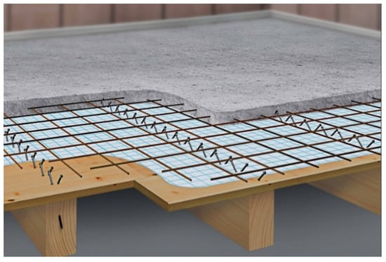
Figure 1.
Wood–concrete composite floors—scheme.
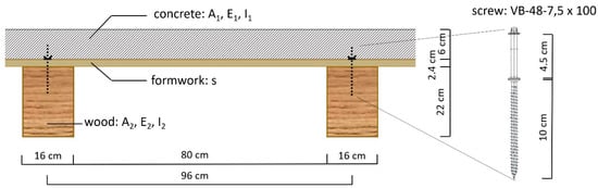
Figure 2.
Cross-section dimensions.
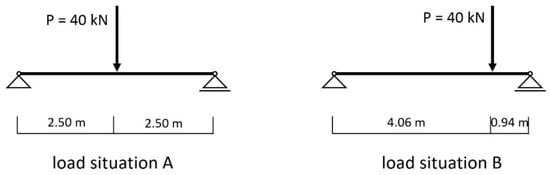
Figure 3.
Load situations.
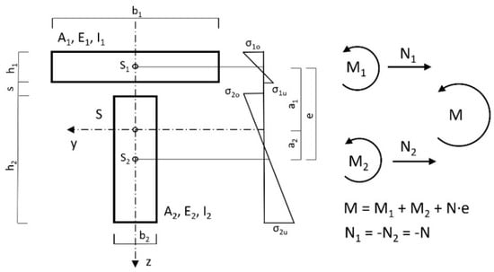
Figure 4.
Idealised cross-section with static parameters.

Table 1.
Characteristic values.
For the “SFS composite screw crossed” fastener, the following displacement moduli were applied according to approval [29]:
Kser = 166 KN/cm for the calculation of the serviceability limit state.
Ku = 2/3 … Kser = 111 KN/cm for the calculation of the ultimate limit state.
The screws, arranged crosswise, were anchored with a length of 100 mm in the wood and 45 mm in the concrete. The bolt heads were located in the concrete in the area of the steel reinforcement. The displacement modulus was a compliance coefficient analogous to the modulus of elasticity, where it corresponded to the proportionality factor in the point and to the linear load-displacement law of the fastener in the contact joint direction. In the differential equation method, the joint stiffness (K) is also important. This was calculated as the quotient of the displacement modulus K (Kser for the deformations and Ku for the forces) divided by the fastener spacing e’ (displacement modulus notionally smeared over the bolt spacing). The fastener spacing in the longitudinal direction of the beam was e’ = 11.1 cm, which resulted from 45 sections for the span of 500 cm.
3. Theory and Calculation
3.1. Calculation of Force Quantities with the Discrete Method
In the method first presented by Stüssi [26,27], the fasteners were represented on the idealised structural model as point-acting single dowels with linear elastic deformation laws (transverse to the joint). Likewise, linear material laws and the validity of the Bernoulli hypothesis were assigned to the concrete belt bar and the timber beam for the individual cross-sections (but not for the total cross-section). Thus, there was an internal highly statically indeterminate structure, with the excess dowel forces acting horizontally in the connection joint (Figure 5). For further consideration, the system was split up and, according to the superposition principle, superimposed on the composite-free girder—each loaded with the dowel forces (acting in the gravity line of the contact joint) and the external load.
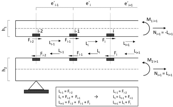
Figure 5.
Exposed composite beam with cutting forces.
Li corresponds to the dowel-force resultant, calculated field by field from the support. The relationship between the dowel-force resultant and the section-normal force is shown in Figure 4. In the belt, for equilibrium reasons, Ni = −Li, while in the web Ni = Li, applies. Using the main bending equation and the material law, length changes in the contact joint due to the affected dowel-force resultants and partial moments (respectively due to the external load and due to the dowel forces) can be calculated.
3.1.1. Partial Moments Due to the External Load
Due to the relatively simple conditions at the unbonded beam, the partial moments due to the external load can be expressed by the total moment M. Following Figure 4, the absence of partial-normal forces means that (N1 = N2 = 0) is valid for the unbonded beam for this load case:
Due to the equal deflections of belt and web (effects due to the twisting of the cross-section were not taken into account), whereby for any beam location w1 = w2, after differentiating twice and neglecting the shear deformation, the geometric compatibility condition follows this equation:
Thus, two equations are available for the two unknowns (M1 and M2), and the task can be solved mathematically and unambiguously if the total moment M is known, whereby the partial moments can be expressed by the total moment. The total moment M0m, averaged over the section, was used to determine the elongation changes.
3.1.2. Partial Moments According to Dowel Forces
The partial moment curve due to the dowel forces is constant in sections.
3.1.3. Compatibility Condition
The fulfilment of the constraint condition, according to Figure 6 and Equation (3), leads directly to Equation (4), which can be set up for each field.
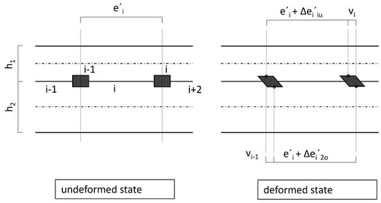
Figure 6.
Continuity condition in the contact joint.
In this case:
ei’: Centre distance of dowels in section i in the undeformed or unloaded state.
ei’ + Δei’1u + vi = ei’ + Δei’2o + vi−1 ⇒ Δei’1u + vi = Δei’2o + vi−1
Δei’1u: Length change of the distance ei’ of the dowels at the height of the lower edge fibre of the upper beam 1 due to the forces and moments acting in this section (moments are to be averaged).
vi: Deformation of dowel i in the direction of the contact joint due to dowel force Fi.
Δei’2o: Change in the length of the distance ei’ of the dowels at the level of the upper edge fibre of the lower beam 2 due to forces and moments acting in this section.
vi−1: Deformation of the dowel i-1 in the direction of the contact joint due to the dowel force Fi−1.
where M0im is the mean total moment in section i. With 45 sections, this results in a system of equations with 45 equations and 45 unknown dowel-force resultants (Li) or partial-normal forces (Ni).
In matrix notation, it follows:
In the matrix, the diagonal value c corresponds to the constant bracket expression on the left side in Equation (4). The factor c is independent of the load, and depends on, among other things, the displacement modulus. The right column vector of the equation system (m1 to m45) also includes the load-case-dependent total moment curve (mi) of the bondless basic system. Due to the special problem definition, with two load cases and one displacement modulus each for the load-bearing capacity and the deformations, a total of four equation systems must be solved.
The numerical evaluations of the four possible combination cases lead to partial-normal forces in the joint. Figure 7 shows this for load-bearing capacity (the shape for the calculation of the deformations is similar). These correspond to the dowel-force resultants, accordingly sign-weighted as already described (belt: −, web: +). In the case of load situation A, the numerically calculated dowel-force resultants/partial-normal forces of the individual beam sections were distributed symmetrically over the beam length, whereas in load situation B, they were distributed asymmetrically due to the different partial moment distribution.
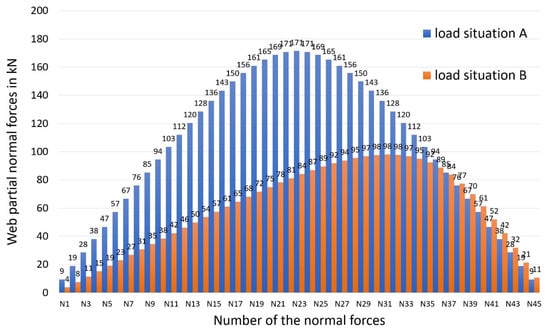
Figure 7.
Web partial-normal forces for the load-bearing capacity.
Furthermore, the partial moments for the real system were obtained directly from this in accordance with Figure 5, with compound use of the following equations (Superposition principle):
where s is the thickness of the formwork according to Figure 2. The results are summarised for the force application point (in the centre of the field for load situation A and 0.94 m distance from the right bearing point for load situation B) in Table 2.
Table 2.
Results according to the discrete method.
3.2. Derivation of Deformations for the Discrete Method
In ref. [28], a proposal for the determination of deflections based on the “principle of virtual forces” was developed for the discrete method. Here again, the “superposition principle” was used as previously described.
According to the working principle, the auxiliary system (one-system) was again the unbonded beam with a load of 1 at the point and in the direction where the deflection was sought.
The respective moment curves in the belt and web were then to be superimposed according to Equation (7), whereby the deflection components due to shear forces were neglected.
The following Figure 8 illustrates the procedure using the example of a single-span beam with a point load in the centre of the span. For the total deflection, the individual deflection components must be added.
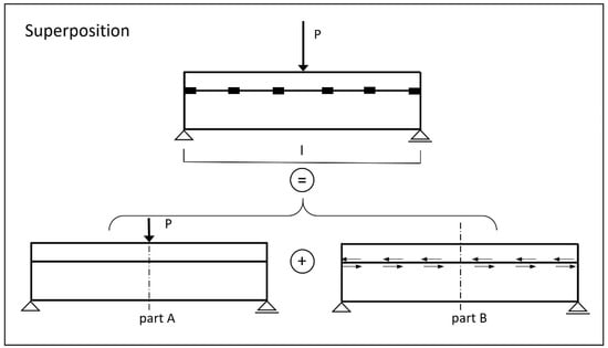
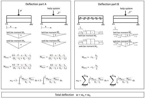
Figure 8.
Procedure for determining deflections with principle of virtual forces.
The deflection at the point of force application (centre of the field for load situation A) resulted in 1.66 cm for load situation A and 0.69 cm for eccentric-load situation B, using the method described and including the numerically determined partial-normal force results according to Figure 8.
3.3. Calculation of Force Quantities and Deformations with the Differential Equation Method
The derivation and solution of the differential equations were carried out by Natterer and Hoeft [25]. The basis for the derivation of the required additional governing equations for the internally statically indeterminate problem (again assuming linear material laws for the composite partners, including the connecting means and the validity of the flatness of the partial cross-sections after bending) was again the fulfilment of the constraint condition in the contact joint of an infinitesimal beam element (dx) with a continuous connection between concrete and wood. This leads to a differential equation system for the contact joint displacement (u) and the beam deflection (w). In a publication [25] of March 1987, the differential equation system was solved for the most common loading situations, leading to continuous governing equations for the mechanical parameters.
In the following, the main equations and preliminary values for the calculation of a single-span beam with concentrated load are presented, where Φ indicates the location of the concentrated load with respect to the span (Figure 9).
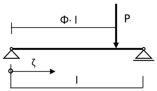
Figure 9.
Load situation.
For the load position (single load at the centre of the field), Φ = 0.5, and the location of the sought mechanical quantities can be expressed by the related bar length variable ζ = 0.5.
In order to simplify the application of the equations of determination, the following preliminary values must be determined (Figure 4 and Table 1 are valid) according to [25]:
The normal force and the bending moments result in:
Table 3 summarises the results of the calculations.
Table 3.
Results according to the differential equation method.
To illustrate and better classify the results, the fictitious case of a rigid bond between wood and concrete was also calculated using this method, and the results are presented in Table 4.
Table 4.
Results for the rigid bond.
According to [25], the deflections were given by Equation (17) for load situation A as 1.68 cm and for load situation B as 0.71 cm. In comparison, the deflections under the assumption of a rigid composite would be calculated as 1.07 cm for load situation A and 0.40 cm for load situation B.
3.4. Gamma Method
Usually, the gamma method is used for composite structures. This is a simple calculation method, which is also the standard method in Eurocode 5 [24]. The advantage lies in compact and easy-to-use formulas, whereby the effective bending stiffness of the entire beam can be used for deformation calculations. With the introduction of an effective moment of inertia, the requirement that the curvature of the individual parts must correspond to the curvature of the entire beam is again met for the composite-free case in an extended sense.
The comparative elastic modulus Ev can be free selected; mostly, Ev = E2 is selected.
Thus, for the effective moment of inertia after some transformation
In the case of a rigid compound, the Steiner component also appears. In the compound-less case (no Steiner part is effective), this corresponds to a weight of the Steiner part of 0. All cases of the real compound can therefore be classified between these two cases (with gamma as a weighting factor = 0 to 1).
The γ-value was obtained by comparing the terms of the gamma method with those of the differential equation method. Compact terms were obtained only for sinusoidal loads, but large and complicated terms were obtained for uniform loads and symmetrically concentrated loads. According to [3], the following formulas result for the sinusoidal load:
where f is an auxiliary value. With the arbitrary comparative elasticity modulus Ev, the effective moment of inertia can be calculated:
For the total moment for load situation A:
and for load situation B:
The partial moments M1 and M2, as well as the normal force, result in
This results in the values compiled in Table 5:
Table 5.
Results according to the gamma method.
The deflections can be determined with the conventional formulas of structural analysis, namely with the effective bending stiffness according to the gamma method in the denominator. Load situation A for x = l/2 follows:
and for the load situation B for x = 0.94
This results in 1.65 cm for load situation A and 0.62 cm for load situation B.
4. Comparison of the Results
Figure 10, Figure 11 and Figure 12 show a comparison of the bending moments M1 and M2 and the normal forces N, and Figure 13 shows the stresses.
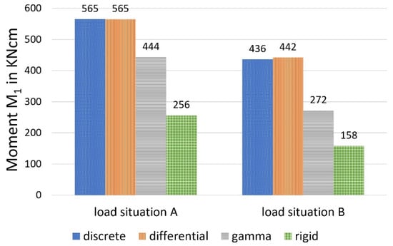
Figure 10.
Moment M1, calculated with different methods.
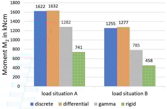
Figure 11.
Moment M2, calculated with different methods.
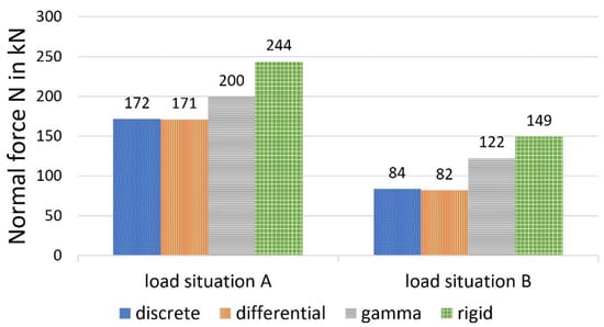
Figure 12.
Normal force N, calculated with different methods.
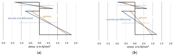
Figure 13.
Longitudinal stresses for load situation A (a) and load situation B (b).
It should first be noted that, under the given conditions, the differential equation method and the discrete method provide almost identical values for the selected load-bearing behaviour variables. This circumstance can be explained by the relatively dense arrangement of the bolt pairs, which creates an almost continuous bond between the wood and the concrete. The sectionally constant moments and normal forces of the discrete method deviate only slightly from the continuous lines of the differential equation method at small distances (here, 45 fields). In contrast to screws, which are always arranged relatively closely, larger distances are present in the case of cleats. In [20], comparative calculations with cleats, which formed only 10 sections (and single loads), were carried out, and also showed deviations between the methods.
As shown in the comparative calculation, the gamma method underestimates more accurate methods with respect to stress determination for both load situations. For load situation A, the gamma method calculates a difference of about minus 13 per cent for σ1o (based on the values calculated with the more stringent method) and minus 11 per cent for σ2u. For load situation B, the differences were even greater (minus 25 per cent for the upper stress versus minus 21 per cent for the lower stress).
This can be explained primarily by a redistribution of the internal forces in the direction of the rigid composite, which was more pronounced in load situation B, according to the data available here. Use of the gamma method leads to a reduction of around 22 per cent for load situation A (minus 39 per cent in load situation B) in the case of the two partial moments, compared with the more stringent methods, with a simultaneous increase in the partial-normal-force stress of 18 per cent (plus 49 per cent in load situation B). This allows the conclusion that, in the case of the central concentrated load and with increasing deviation from this, the gamma method underestimates the bending stress and overestimates the partial-normal-force stress. The values, therefore, erroneously approach the exact results assuming a rigid composite. This was also ultimately reflected in the deflections (in particular load situation B, with minus 11 per cent).
The deflections, shown in Figure 14, are approximately the same for all 3 calculation models and larger than with the rigid system.
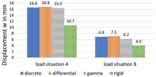
Figure 14.
Deflection w, calculated with different methods.
5. Conclusions
In summary, the gamma method is to be considered as a model-rate inaccurate method for the computational determination of two-part wood–concrete hybrid beams with common design features, especially for predominantly eccentrically located load situations compared to the more stringent method.
The gamma method underestimates the stress and deformation quantities to be determined for both the ultimate limit state design and the serviceability check, and is therefore on the unsafe side.
From a design point of view, the differences can, in any case, become decisive with regard to an exact verification, and thus represent a design-relevant criterion under certain conditions. Deviations can also occur with a larger spacing of the cleats—even with uniform loads—as described in [20]. In view of these results, it is therefore recommended to use the more stringent differential equation method for mathematical prediction in such exceptional situations.
In summary, it is to be stated that the discrete method, which involves a high computational effort, is a valuable methodology for the accurate simulation of conventional wood–concrete composite beams, especially in the case of single loads.
Author Contributions
Conceptualisation, C.H. and K.D.; methodology, C.H.; software, C.H. and K.D.; validation, C.H. and K.D., formal analysis, C.H.; writing—original draft preparation, C.H.; writing—review and editing, K.D.; visualisation, K.D.; project administration K.D. All authors have read and agreed to the published version of the manuscript.
Funding
This research received no external funding.
Institutional Review Board Statement
Not applicable.
Informed Consent Statement
Not applicable.
Data Availability Statement
Not applicable.
Acknowledgments
Open Access Funding by TU Wien.
Conflicts of Interest
The authors declare no conflict of interest.
References
- Holschemacher, K.; Selle, R.; Schmidt, J.; Kieslich, H. Wood-Concrete-Composite; Betonkalender: Berlin, Germany, 2013; pp. 241–287. (In German) [Google Scholar]
- Yeoh, D.; Fragiacomo, M.; de Franceschi, M.; Boon, K.H. State of the Art on Timber-Concrete Composite Structures: Literature Review. J. Struct. Eng. 2011, 137, 1085–1095. [Google Scholar] [CrossRef]
- Grosse, M.; Rautenstrauch, K. Numerical modelling of timber and connection elements used in timber-concrete-composite constructions. Edinburgh 2004, 17, CIB-W18/37-7-15. [Google Scholar]
- Kolbitsch, A.; Pauser, A.; Bölcskey, E.; Zajicek, P. Reinforcement of Existing Wooden Ceilings with Consideration of Subsequently Manufactured Wood-Concrete Composite Structures, Research Project F 1021—Part Wooden Ceiling Structures; Österreichische Gesellschaft zur Erhaltung von Bauten: Wien, Austria, 1992. (In German) [Google Scholar]
- Grosse, M.; Hartnack, R.; Lehmann, S.; Rautenstrauch, K. Modeling of discontinuously connected wood-concrete composite slabs/Part 1: Short-term behavior. Bautechnik 2003, 80, 534–541. (In German) [Google Scholar] [CrossRef]
- Kuhlmann, U.; Schänzlin, J.; Michelfelder, B. Calculation of wood-concrete composite floors. Beton-Und Stahlbetonbau 2004, 99, 262–270. (In German) [Google Scholar] [CrossRef]
- Grosse, M.; Hartnack, R.; Rautenstrauch, K. Modeling of discontinuously connected wood-concrete composite slabs/Part 2: Long-term behavior. Bautechnik 2003, 80, 693–701. (In German) [Google Scholar] [CrossRef]
- Avak, R.; Glaser, R. Simplified method for predicting the long-term behavior of wood-concrete composite structures. Bautechnik 2005, 82, 200–211. (In German) [Google Scholar] [CrossRef]
- Gerold, M.; Schänzlin, J.; Kuhlmann, U. Wood as an ideal composite partner for concrete as a building material. Bautechnik 2003, 80, 840–845. (In German) [Google Scholar] [CrossRef]
- Schmidt, J.; Schneider, W.; Thiel, R. To design wood/concrete composite beams. Bautechnik 2003, 80, 302–309. (In German) [Google Scholar] [CrossRef]
- Schmidt, J.; Kaliske, M.; Schneider, W.; Thiele, R. Design proposal for wood/concrete composite beams considering graded fastener spacings. Bautechnik 2004, 81, 172–179. [Google Scholar] [CrossRef]
- Rautenstrauch, K.; Grosse, M.; Lehmann, S.; Hartnack, R. Practical dimensioning of wood-concrete composite floors, 6. Informationstag des IKI; Bauhaus Universität Weimar: Weimar, Germany, 2003. (In German) [Google Scholar]
- Forsberg, A.; Farbäck, F. Timber Concrete Composite Floors with Cross Laminated Timber—Structural Behaviour & Design, Division of Structural Engineering, Faculty of Engineering; Report TVBK-20/5279; Lund University: Lund, Sweden, 2020. [Google Scholar]
- Wallner-Novak, M.; Koppelhuber, J.; Pock, K. Cross-Laminated Timber Structural Design|Basic Design and Engineering Principles According to Eurocode; Proholz: Vienna, Austria, 2014. (In German) [Google Scholar]
- Heller, H. Wood-concrete composite floors (HBV). Bautechnik 2008, 85, 667–677. (In German) [Google Scholar] [CrossRef]
- Schröter, H.; Simon, A.; Timmler, H.-G.; Rautenstrauch, K.; Raue, E. For the calculation of wood-concrete composite beams with methods of mathematical optimization. Bautechnik 2010, 87, 474–481. (In German) [Google Scholar]
- Schäfers, M.; Seim, W. Bonded composite components made of wood and high-strength and ultra-high-performance. Bautechnik 2011, 88. (In German) [Google Scholar]
- Grosse, M.; Rautenstrauch, K.; Schlegel, R. Numerical modeling of wood and fasteners in wood-concrete composite structures. Bautechnik 2005, 82, 355–364. (In German) [Google Scholar] [CrossRef]
- Schönborn, F.; Flach, M.; Feix, J. Design rules and design information for shear collars in wood-concrete composite structures. Beton-Und Stahlbetonbau 2011, 106, 385–393. (In German) [Google Scholar] [CrossRef]
- Woschitz, R.; Deix, K.; Huber, C.; Kampitsch, T. Development of innovative wood-concrete composite slabs in prefabricated construction method. Bautechnik 2021, 98, 12–22. (In German) [Google Scholar] [CrossRef]
- Dias, A.; Schänzlin, J.; Dietsch, P. Design of Timber-Concrete Composite Structures; Shaker Verlag GmbH: Aachen, Germany, 2018. [Google Scholar] [CrossRef]
- Möhler, K. On the Load-Carrying Behavior of Flexural Beams and Compression Members with Composite Cross-Sections and Yielding Connectors; TH Karlsruhe: Karlsruhe, Germany, 1956. (In German) [Google Scholar]
- Heimeshoff, B. To calculate flexural beams made of yieldingly connected cross-section parts in engineered timber construction. Holz Als Roh-Und Werkst. 1987, 45, 237–241. (In German) [Google Scholar] [CrossRef]
- ÖNORM EN 1995-1-1, Eurocode 5. Designs of Timber Strutures, Part 1-1: General—Common Rules and Rules for Buildings; Austrian Standards: Vienna, Austria, 2019. [Google Scholar]
- Natterer, J.; Hoeft, M. The Load-Bearing Behavior of Wood-Concrete Composite Structures; Forschungsbericht CERS Nr. 1345; EPFL/IBOIS: Lausanne, Switzerland, 1987. (In German) [Google Scholar]
- Stüssi, F. About the doweled beam. Schweiz. Bauz. 1943, 122, 271–274. (In German) [Google Scholar]
- Stüssi, F. Composite Solid Wall Beams; Abhandlung der Int. Ver. für Brückenbau und Hochbau: Zürich, Switzerland, 1947; pp. 249–268. [Google Scholar]
- Huber, C. Document on the Design of Wood-Concrete Composite Floors with Selected Fasteners under Fire Exposure; Institut für Hochbau und Technologie TU Wien: Vienna, Austria, 2010. (In German) [Google Scholar]
- Zulassungsnummer Z-9.1-342. SFS-Compound Screws, VB-48-7,5x100 as a Fastener for the SFS Wood-Concrete Composite System; Allgemeine Bauaufsichtliche Zulassung: Berlin, Germany, 2003. (In German) [Google Scholar]
Publisher’s Note: MDPI stays neutral with regard to jurisdictional claims in published maps and institutional affiliations. |
© 2021 by the authors. Licensee MDPI, Basel, Switzerland. This article is an open access article distributed under the terms and conditions of the Creative Commons Attribution (CC BY) license (https://creativecommons.org/licenses/by/4.0/).