Feasibility of Machine Learning Algorithms for Predicting the Deformation of Anodic Titanium Films by Modulating Anodization Processes


Abstract
:1. Introduction
2. Experimental Dataset Development
3. Machine Learning Algorithm Development
3.1. Data Preprocessing for Classification
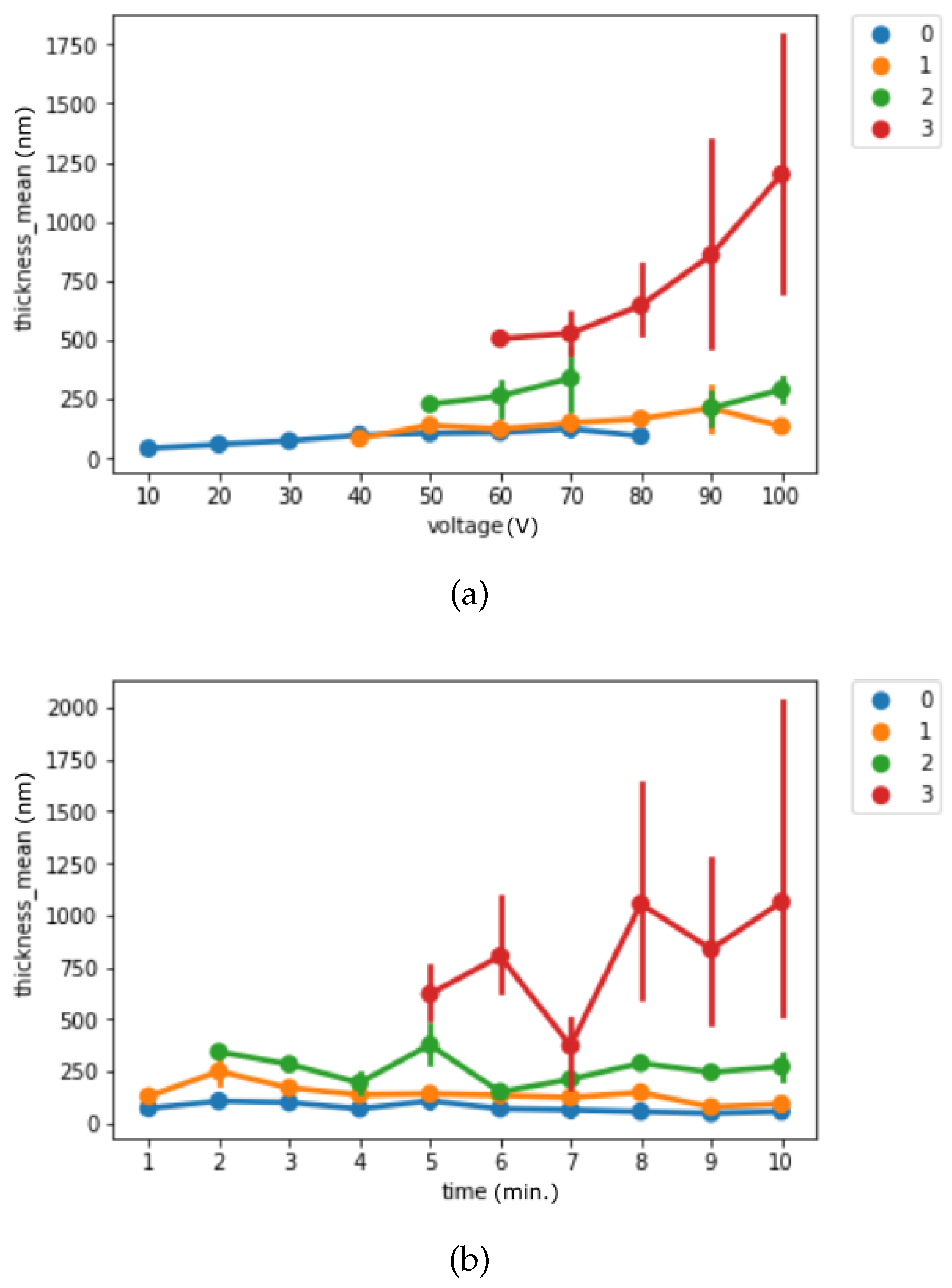
- Class 0: oxide layer creation
- Class 1: oxide layer creation with roughness
- Class 2: oxide layer creation with pore creation
- Class 3: oxide layer creation with uniform pore generation
3.2. Classification Algorithms
3.3. Performance Measures for Machine Learning Algorithms
3.3.1. Binary Classification
3.3.2. Multiclass Classification
4. Results
4.1. Experiment Results
4.2. Change of Thickness
4.3. Classification Results
4.3.1. Prediction on Binary Classification
4.3.2. Multiclass Classification
5. Discussion
6. Conclusions
Author Contributions
Funding
Institutional Review Board Statement
Informed Consent Statement
Data Availability Statement
Conflicts of Interest
References
- Byon, E.; Moon, S.; Cho, S.B.; Jeong, C.Y.; Jeong, Y.; Sul, Y.T. Electrochemical property and apatite formation of metal ion implanted titanium for medical implants. Surf. Coatings Technol. 2005, 200, 1018–1021. [Google Scholar] [CrossRef]
- Fujishima, A.; Honda, K. Electrochemical photolysis of water at a semiconductor electrode. Nature 1972, 238, 37–38. [Google Scholar] [CrossRef] [PubMed]
- Xie, Z.; Adams, S.; Blackwood, D.; Wang, J. The effects of anodization parameters on titania nanotube arrays and dye sensitized solar cells. Nanotechnology 2008, 19, 405701. [Google Scholar] [CrossRef]
- Zhang, Y.; Li, X.; Hua, X.; Ma, N.; Chen, D.; Wang, H. Sunlight photocatalysis in coral-like TiO2 film. Scr. Mater. 2009, 61, 296–299. [Google Scholar] [CrossRef]
- Jeong, C.; Choi, C.H. Single-step direct fabrication of pillar-on-pore hybrid nanostructures in anodizing aluminum for superior superhydrophobic efficiency. Acs Appl. Mater. Interfaces 2012, 4, 842–848. [Google Scholar] [CrossRef]
- Minagar, S.; Berndt, C.C.; Wang, J.; Ivanova, E.; Wen, C. A review of the application of anodization for the fabrication of nanotubes on metal implant surfaces. Acta Biomater. 2012, 8, 2875–2888. [Google Scholar] [CrossRef]
- Smith, B.S.; Yoriya, S.; Johnson, T.; Popat, K.C. Dermal fibroblast and epidermal keratinocyte functionality on titania nanotube arrays. Acta Biomater. 2011, 7, 2686–2696. [Google Scholar] [CrossRef] [PubMed]
- Yoo, S.Y.; Park, H.G. Effect of anodic oxidation process parameters on TiO2 nanotube formation in Ti-6Al-4V Alloys. Korean J. Met. Mater. 2019, 57, 521–528. [Google Scholar] [CrossRef]
- Miao, Z.; Xu, D.; Ouyang, J.; Guo, G.; Zhao, X.; Tang, Y. Electrochemically induced sol- gel preparation of single-crystalline TiO2 nanowires. Nano Lett. 2002, 2, 717–720. [Google Scholar] [CrossRef]
- Sander, M.S.; Cote, M.J.; Gu, W.; Kile, B.M.; Tripp, C.P. Template-assisted fabrication of dense, aligned arrays of titania nanotubes with well-controlled dimensions on substrates. Adv. Mater. 2004, 16, 2052–2057. [Google Scholar] [CrossRef]
- Jeong, C.; Ji, H. Systematic control of anodic aluminum oxide nanostructures for enhancing the superhydrophobicity of 5052 aluminum alloy. Materials 2019, 12, 3231. [Google Scholar] [CrossRef] [PubMed] [Green Version]
- Ji, H.; Jeong, C. Study on corrosion and oxide growth behavior of anodized aluminum 5052 Alloy. J. Korean Inst. Surf. Eng. 2018, 51, 372–380. [Google Scholar]
- Chen, X.; Selloni, A. Introduction: Titanium dioxide (TiO2) nanomaterials. Chem. Rev. 2014, 114, 9281–9282. [Google Scholar] [CrossRef] [PubMed]
- Lee, B.; Lee, S.; Choi, J.; Jeong, Y.; Oh, H.J.; Lee, O.Y.; Chi, C.S. Growth behaviors of anodic titanium oxide nanotubes in the ethylene glycol solution according to water contents. J. Korean Inst. Met. Mater. 2008, 46, 700–706. [Google Scholar]
- Macák, J.M.; Tsuchiya, H.; Schmuki, P. High-aspect-ratio TiO2 nanotubes by anodization of titanium. Angew. Chem. Int. Ed. 2005, 44, 2100–2102. [Google Scholar] [CrossRef]
- Diebold, U. The surface science of titanium dioxide. Surf. Sci. Rep. 2003, 48, 53–229. [Google Scholar] [CrossRef]
- Henderson, M.A. A surface science perspective on TiO2 photocatalysis. Surf. Sci. Rep. 2011, 66, 185–297. [Google Scholar] [CrossRef]
- Kukovecz, Á.; Kordás, K.; Kiss, J.; Kónya, Z. Atomic scale characterization and surface chemistry of metal modified titanate nanotubes and nanowires. Surf. Sci. Rep. 2016, 71, 473–546. [Google Scholar] [CrossRef] [Green Version]
- Jeong, C.; Lee, J.; Sheppard, K.; Choi, C.H. Air-impregnated nanoporous anodic aluminum oxide layers for enhancing the corrosion resistance of aluminum. Langmuir 2015, 31, 11040–11050. [Google Scholar] [CrossRef]
- Kulkarni, M.; Mazare, A.; Schmuki, P.; Iglic, A. Influence of anodization parameters on morphology of TiO2 nanostructured surfaces. Adv. Mater. Lett. 2016, 7, 23–28. [Google Scholar] [CrossRef] [Green Version]
- Alpaydin, E. Introduction to Machine Learning; MIT Press: Cambridge, MA, USA, 2020. [Google Scholar]
- Liu, Y.; Zhao, T.; Ju, W.; Shi, S. Materials discovery and design using machine learning. J. Mater. 2017, 3, 159–177. [Google Scholar] [CrossRef]
- Fan, R.E.; Chang, K.W.; Hsieh, C.J.; Wang, X.R.; Lin, C.J. LIBLINEAR: A library for large linear classification. J. Mach. Learn. Res. 2008, 9, 1871–1874. [Google Scholar]
- Saritas, M.M.; Yasar, A. Performance analysis of ANN and Naive Bayes classification algorithm for data classification. Int. J. Intell. Syst. Appl. Eng. 2019, 7, 88–91. [Google Scholar] [CrossRef] [Green Version]
- Nikam, S.S. A comparative study of classification techniques in data mining algorithms. Orient. J. Comput. Sci. Technol. 2015, 8, 13–19. [Google Scholar]
- Chang, C.C.; Lin, C.J. LIBSVM: A library for support vector machines. ACM Trans. Intell. Syst. Technol. 2011, 2, 1–27. [Google Scholar] [CrossRef]
- Liaw, A.; Wiener, M. Classification and regression by RandomForest. R News 2002, 2, 18–22. [Google Scholar]
- Becker, C.; Rigamonti, R.; Lepetit, V.; Fua, P. Supervised feature learning for curvilinear structure segmentation. In International Conference on Medical Image Computing and Computer-Assisted Intervention; Springer: Berlin/Heidelberg, Germany, 2013; pp. 526–533. [Google Scholar]
- Natekin, A.; Knoll, A. Gradient boosting machines, a tutorial. Front. Neurorobot. 2013, 7, 21. [Google Scholar] [CrossRef] [Green Version]
- Myles, A.J.; Feudale, R.N.; Liu, Y.; Woody, N.A.; Brown, S.D. An introduction to decision tree modeling. J. Chemom. J. Chemom. Soc. 2004, 18, 275–285. [Google Scholar] [CrossRef]
- Brownlee, J. Master Machine Learning Algorithms: Discover how They Work and Implement Them from Scratch; Machine Learning Mastery: Cambridge, MA, USA, 2016. [Google Scholar]
- Aly, M. Survey on multiclass classification methods. Neural Netw. 2005, 19, 1–9. [Google Scholar]
- Bengio, Y.; Grandvalet, Y. No unbiased estimator of the variance of k-fold cross-validation. J. Mach. Learn. Res. 2004, 5, 1089–1105. [Google Scholar]
- Liu, Y.; Bi, J.W.; Fan, Z.P. Multi-class sentiment classification: The experimental comparisons of feature selection and machine learning algorithms. Expert Syst. Appl. 2017, 80, 323–339. [Google Scholar] [CrossRef] [Green Version]
- Powers, D.M. Evaluation: From precision, recall and F-measure to ROC, informedness, markedness and correlation. J. Mach. Learn. Technol. 2011, 2, 37–63. [Google Scholar]
- Fawcett, T. ROC graphs: Notes and practical considerations for researchers. Mach. Learn. 2004, 31, 1–38. [Google Scholar]
- Metz, C.E. Basic principles of ROC analysis. In Seminars in Nuclear Medicine; WB Saunders: Philadelphia, PA, USA, 1978; Volume 8, pp. 283–298. [Google Scholar]
- Sokolova, M.; Lapalme, G. A systematic analysis of performance measures for classification tasks. Inf. Process. Manag. 2009, 45, 427–437. [Google Scholar] [CrossRef]
- Su’ait, M.; Alamgir, F.; Scardi, P.; Ahmad, A. Morphological studies of vertical arrays TiO2 nanotubes by electrochemical anodization technique for dye sensitized solar cell application. Am. Inst. Phys. 2013, 1571, 835–842. [Google Scholar]
- Zhang, A.Y.; Long, L.L.; Liu, C.; Li, W.W.; Yu, H.Q. Chemical recycling of the waste anodic electrolyte from the TiO2 nanotube preparation process to synthesize facet-controlled TiO2 single crystals as an efficient photocatalyst. Green Chem. 2014, 16, 2745–2753. [Google Scholar] [CrossRef]
- Lee, K.C.; Sreekantan, S.; Ahmad, Z.A.; Saharudin, K.A.; Taib, M.A.A. Nucleation of octahedral titanate crystals using waste anodic electrolyte from the anodization of TiO2 nanotubes. CrystEngComm 2017, 19, 6406–6411. [Google Scholar] [CrossRef]
- Frery, J.; Habrard, A.; Sebban, M.; Caelen, O.; He-Guelton, L. Efficient top rank optimization with gradient boosting for supervised anomaly detection. In Proceedings of the Joint European Conference on Machine Learning and Knowledge Discovery in Databases, Skopje, Macedonia, 18–22 September 2017; pp. 20–35. [Google Scholar]
- Beleites, C.; Neugebauer, U.; Bocklitz, T.; Krafft, C.; Popp, J. Sample size planning for classification models. Anal. Chim. Acta 2013, 760, 25–33. [Google Scholar] [CrossRef] [Green Version]
- Caruana, R.; Niculescu-Mizil, A. An empirical comparison of supervised learning algorithms. In Proceedings of the 23rd International Conference on Machine Learning, Pittsburgh, PA, USA, 25–29 June 2006; pp. 161–168. [Google Scholar]
- Wettschereck, D.; Dietterich, T.G. An experimental comparison of the nearest-neighbor and nearest-hyperrectangle algorithms. Mach. Learn. 1995, 19, 5–27. [Google Scholar] [CrossRef] [Green Version]


| Binary Class | Without Pore | With Pore | ||
|---|---|---|---|---|
| Multiclass | Class 0 | Class 1 | Class 2 | Class 3 |
| Definition | Only layer | Layer with roughness | Unstable pore | Uniform pore |
| Layer Creation | ◯ | ◯ | ◯ | ◯ |
| Layer with Roughness | ◯ | ◯ | ◯ | |
| Pore Creation | ◯ | ◯ | ||
| Pore with Certain Height | ◯ | |||
| Sample Image | 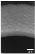 |  | 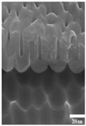 | 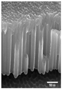 |
| Thickness(nm) | ||||
| # of samples | 50 | 14 | 13 | 23 |
 | |
|---|---|
| A (1 min.) | 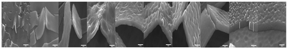 |
| B (2 min.) |  |
| C (3 min.) | 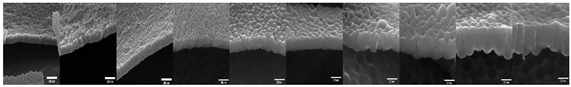 |
| D (4 min.) | 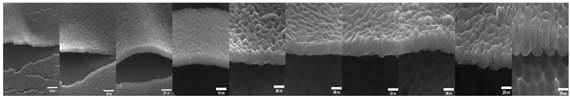 |
| E (5 min.) | 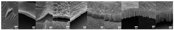 |
| F (6 min.) | 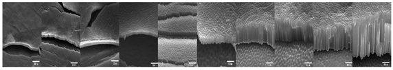 |
| G (7 min.) | 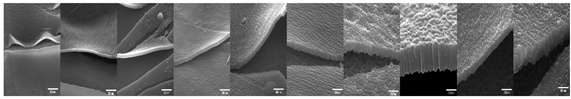 |
| H (8 min.) |  |
| I (9 min.) | 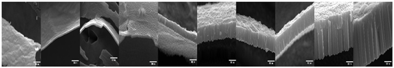 |
| J (10 min.) | 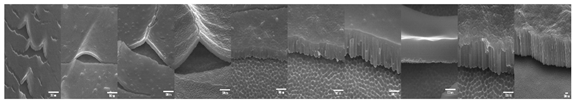 |
| Algorithms | AUC | Accuracy | Precision | Recall |
|---|---|---|---|---|
| LogReg | 0.98 | 0.90 | 0.88 | 0.90 |
| NB | 0.99 | 0.91 | 0.92 | 0.88 |
| KNN | 0.93 | 0.88 | 0.87 | 0.86 |
| SVM | 0.97 | 0.87 | 0.93 | 0.75 |
| DecTree | 0.91 | 0.92 | 0.94 | 0.88 |
| RF | 1.00 | 0.91 | 0.94 | 0.85 |
| Bagging | 0.97 | 0.90 | 0.96 | 0.90 |
| GBT | 1.00 | 0.93 | 0.94 | 0.90 |
| Algorithms | Accuracy | Micro Precision | Micro Recall | Macro Precision | Macro Recall |
|---|---|---|---|---|---|
| LogReg | 0.74 | 0.74 | 0.74 | 0.42 | 0.53 |
| NB | 0.78 | 0.78 | 0.78 | 0.60 | 0.65 |
| KNN | 0.70 | 0.70 | 0.70 | 0.52 | 0.57 |
| SVM | 0.74 | 0.74 | 0.75 | 0.55 | 0.57 |
| DecTree | 0.82 | 0.84 | 0.84 | 0.73 | 0.74 |
| RF | 0.79 | 0.79 | 0.79 | 0.66 | 0.65 |
| Bagging | 0.81 | 0.80 | 0.77 | 0.70 | 0.65 |
| GBT | 0.80 | 0.80 | 0.80 | 0.63 | 0.69 |
Publisher’s Note: MDPI stays neutral with regard to jurisdictional claims in published maps and institutional affiliations. |
© 2021 by the authors. Licensee MDPI, Basel, Switzerland. This article is an open access article distributed under the terms and conditions of the Creative Commons Attribution (CC BY) license (http://creativecommons.org/licenses/by/4.0/).
Share and Cite
Kim, S.-H.; Jeong, C. Feasibility of Machine Learning Algorithms for Predicting the Deformation of Anodic Titanium Films by Modulating Anodization Processes. Materials 2021, 14, 1089. https://doi.org/10.3390/ma14051089
Kim S-H, Jeong C. Feasibility of Machine Learning Algorithms for Predicting the Deformation of Anodic Titanium Films by Modulating Anodization Processes. Materials. 2021; 14(5):1089. https://doi.org/10.3390/ma14051089
Chicago/Turabian StyleKim, Sung-Hee, and Chanyoung Jeong. 2021. "Feasibility of Machine Learning Algorithms for Predicting the Deformation of Anodic Titanium Films by Modulating Anodization Processes" Materials 14, no. 5: 1089. https://doi.org/10.3390/ma14051089
APA StyleKim, S.-H., & Jeong, C. (2021). Feasibility of Machine Learning Algorithms for Predicting the Deformation of Anodic Titanium Films by Modulating Anodization Processes. Materials, 14(5), 1089. https://doi.org/10.3390/ma14051089