
FEM Analysis as a Tool to Study the Behavior of Methacrylate Adhesive in a Full-Scale Steel-Steel Shear Joint


Abstract
:1. Introduction
2. Laboratory Material Testing—Results and Discussion
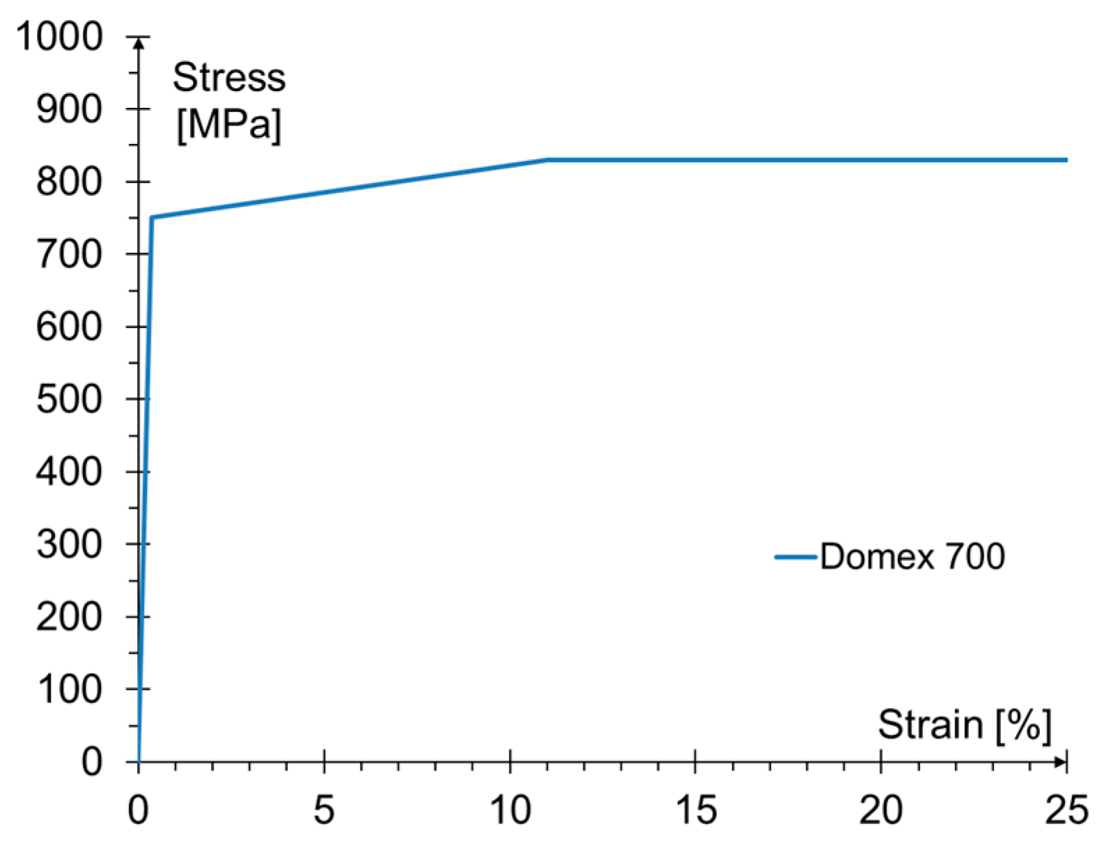
2.1. Steel
2.2. Adhesive
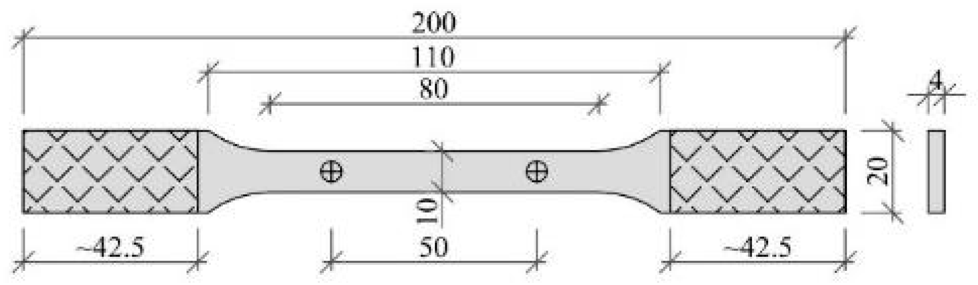
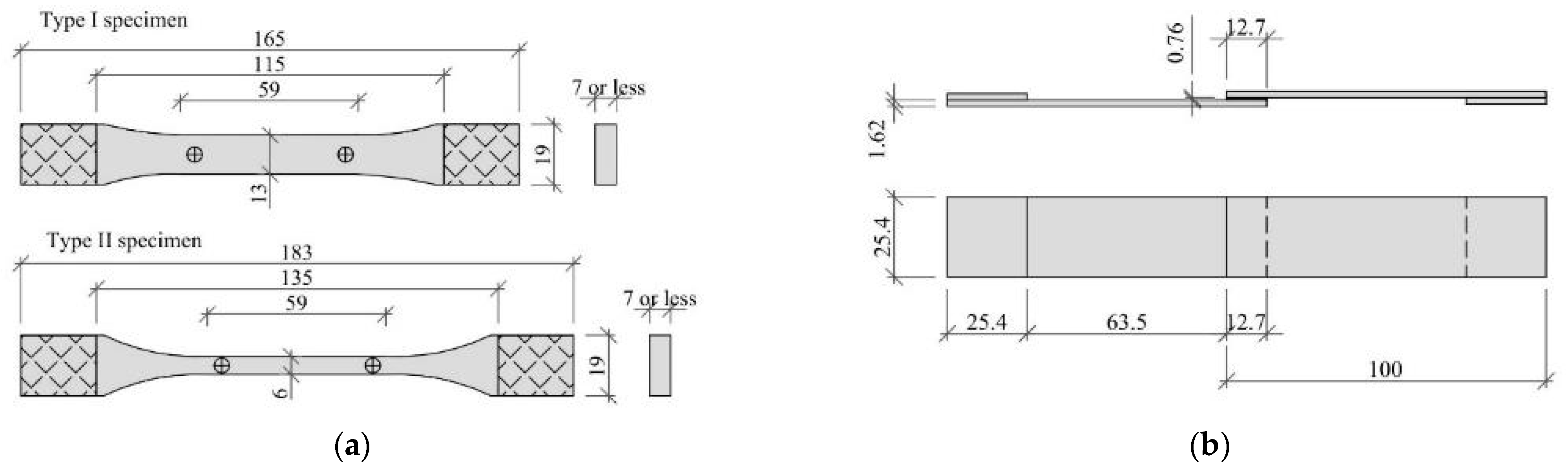
2.2.1. Tensile Strength
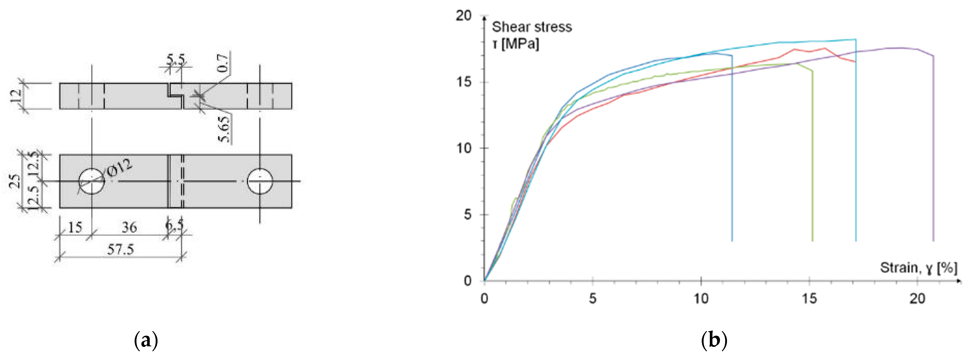
2.2.2. Shear Strength—Single Lap Joint (SLJ)
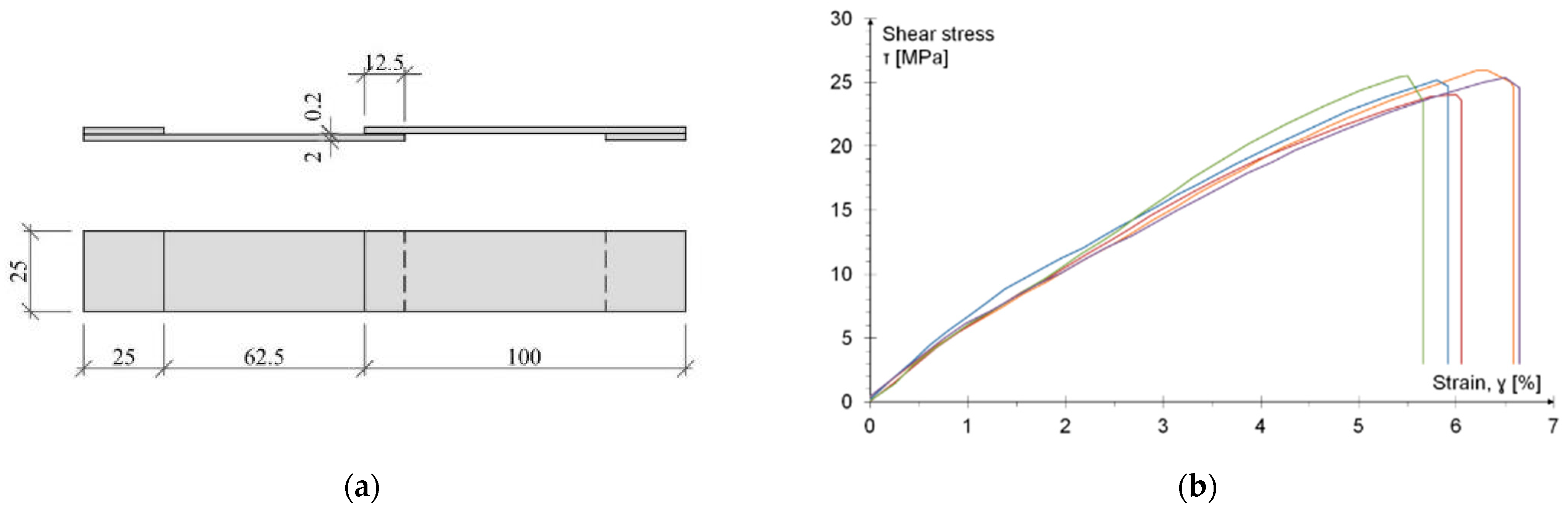
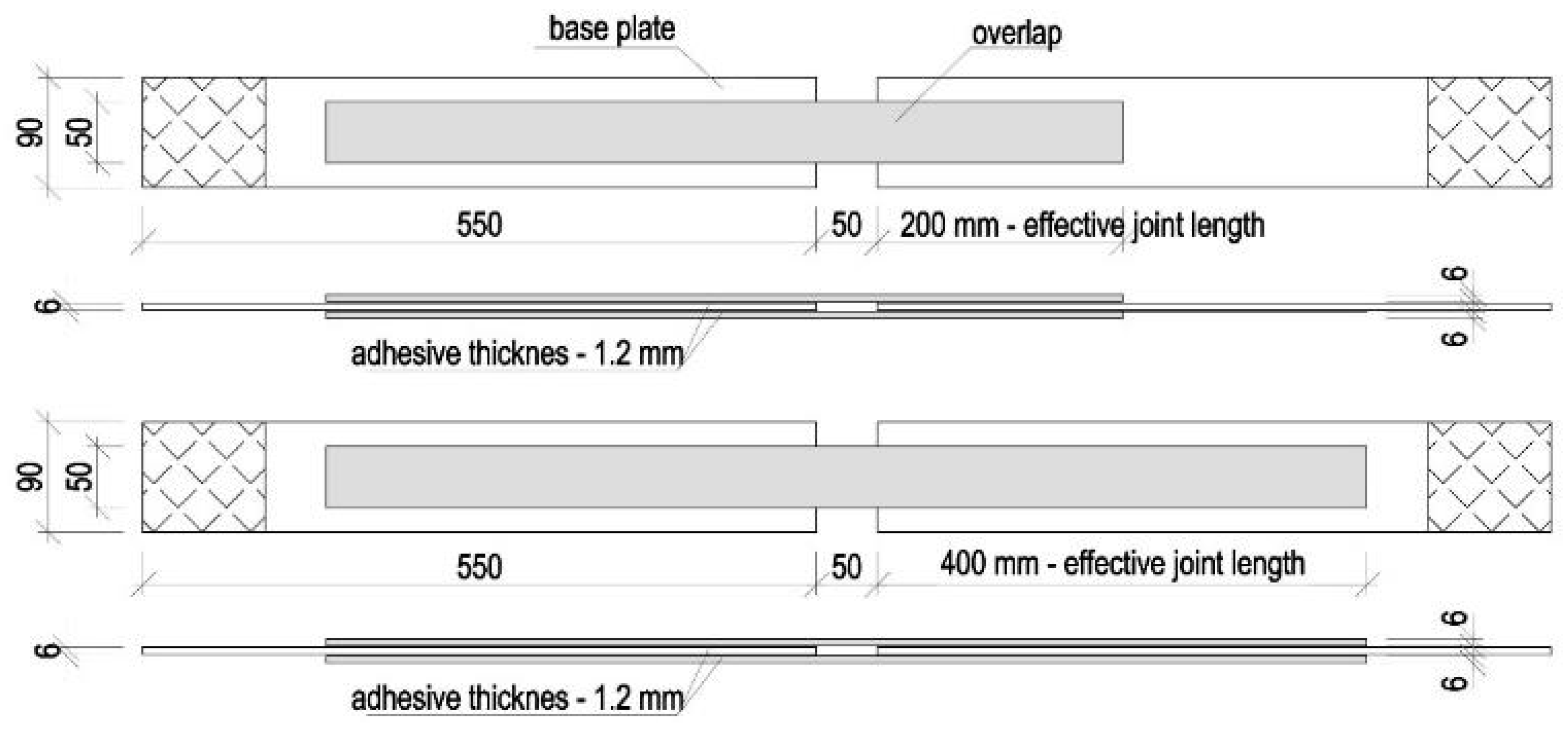
2.2.3. Shear Strength—Thick Adherent Shear Test (TAST)
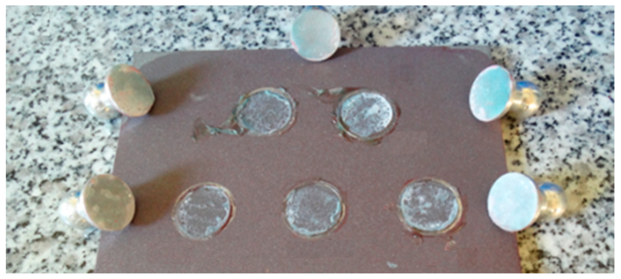
2.2.4. Bond Strength
2.2.5. Analysis and Discussion of Material Test Results
3. Laboratory Model Testing—Results and Discussion
3.1. Testing Procedure
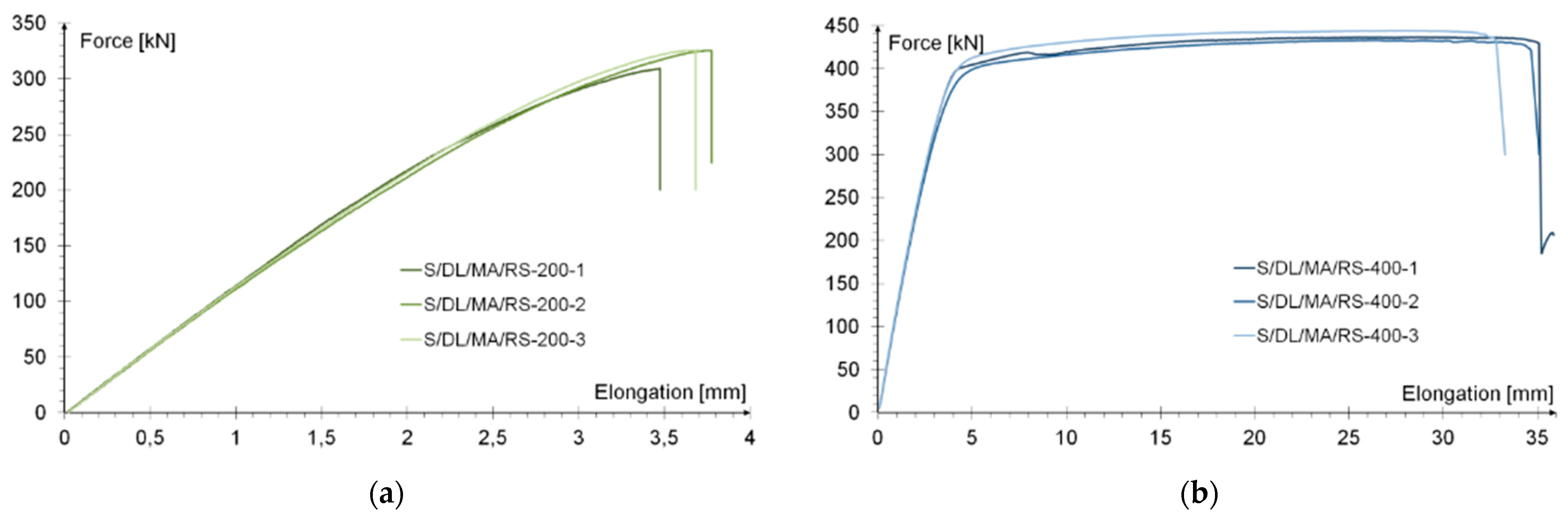
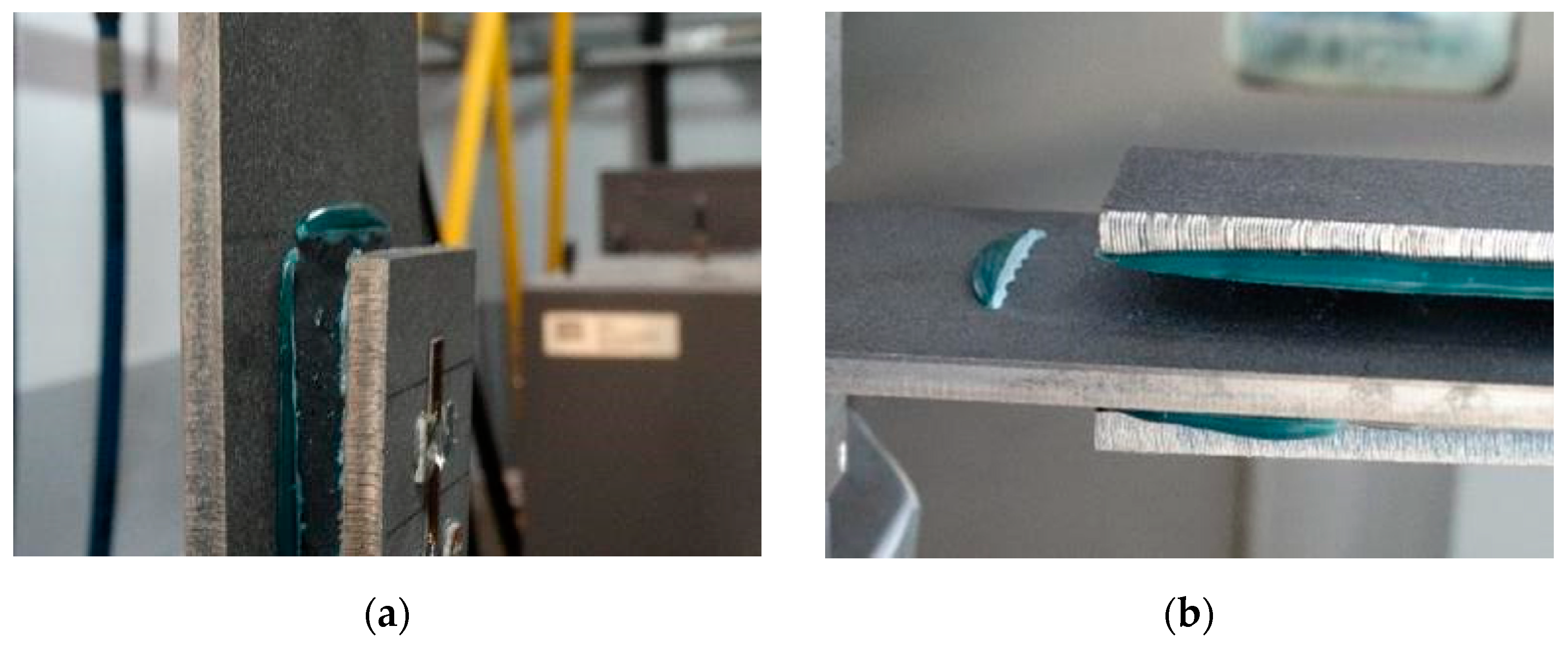
3.2. Results and Discussion
4. Numerical Modeling—Assumption
4.1. Model Selection
4.2. Material Model of the Adhesive
4.2.1. True Values
4.2.2. Continuous Model with Plasticization
4.3. Material Model of the Steel
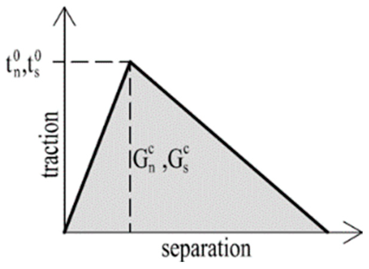
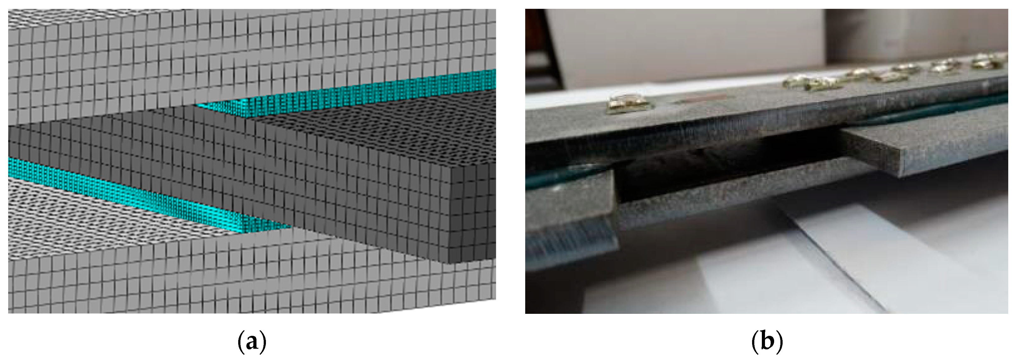
4.4. Contact Layer Model
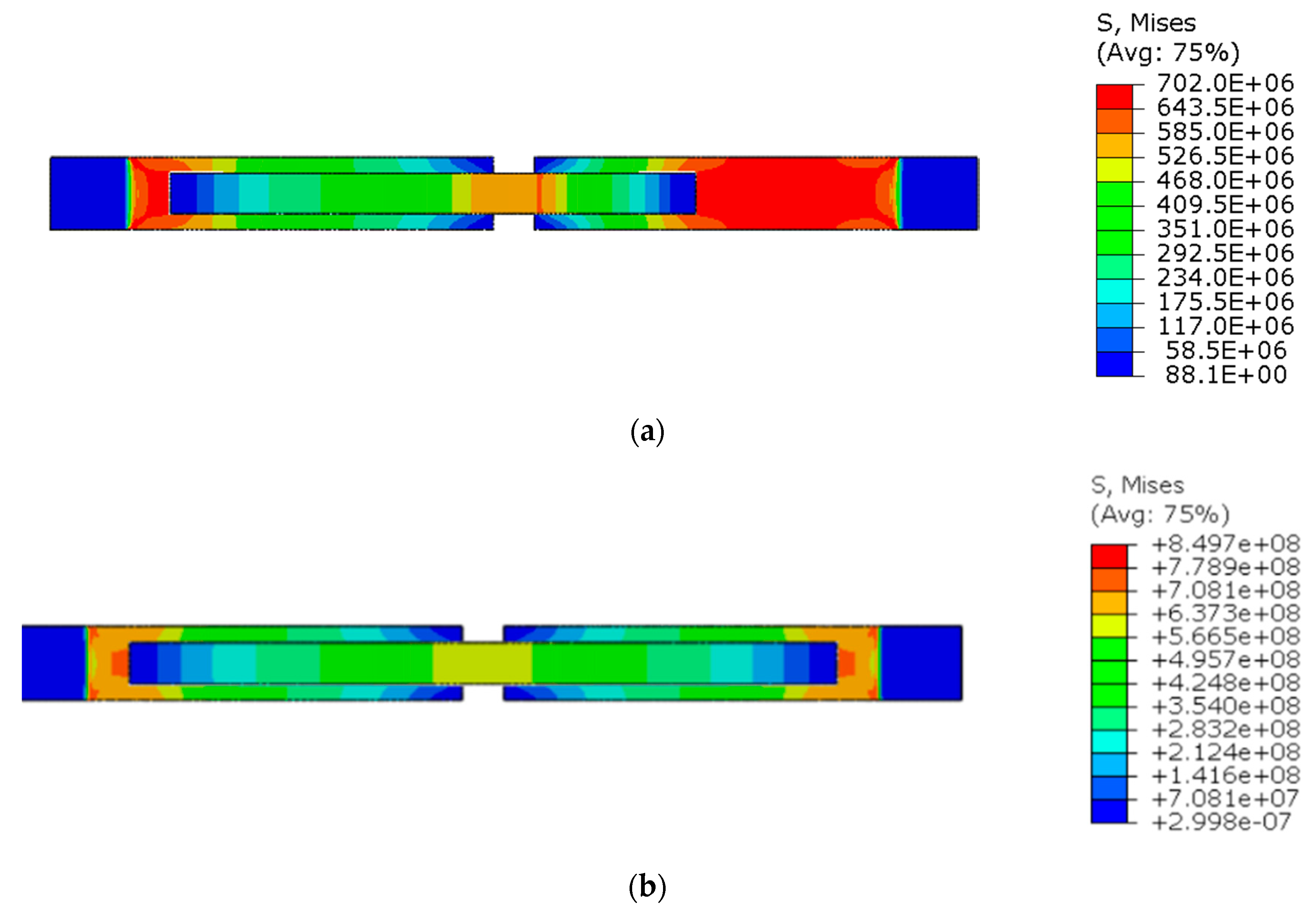
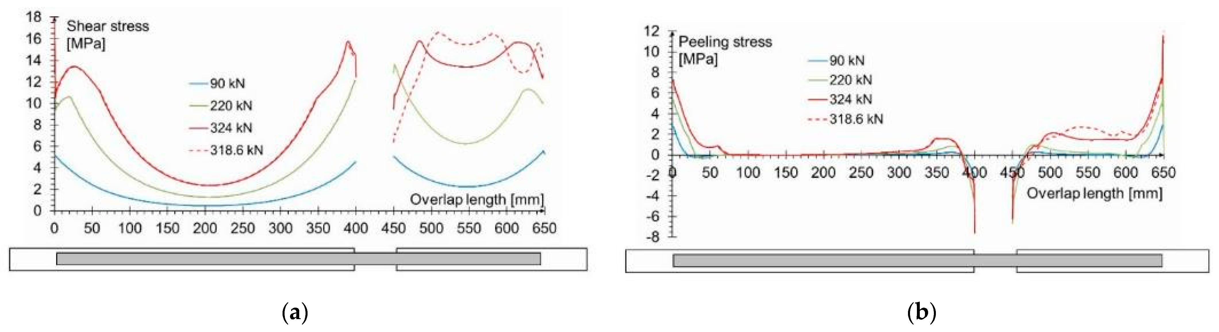
5. Numerical Model—Results and Discussion
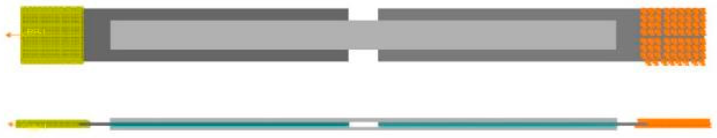
5.1. Characteristic of the Numerical Model
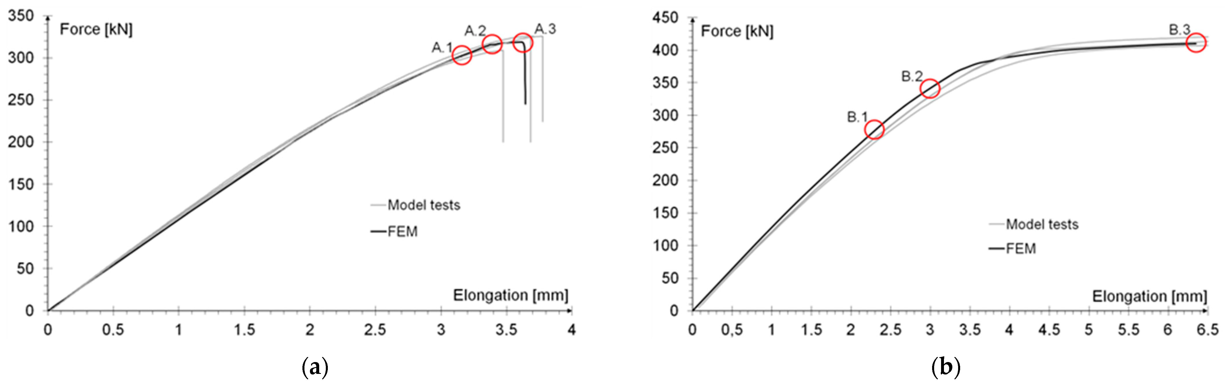
5.2. Nmerical Model Validarion—Discussion
5.3. Deformation Analysis—Discussion
6. Conclusions
Author Contributions
Funding
Institutional Review Board Statement
Informed Consent Statement
Data Availability Statement
Acknowledgments
Conflicts of Interest
References
- McBain, J.W.; Hopkins, D.G. On Adhesives and Adhesive Action. J. Phys. Chem. 1925, 29, 188–204. [Google Scholar] [CrossRef]
- Higgins, A. Adhesive bonding of aircraft structures. Int. J. Adhes. Adhes. 2000, 20, 367–376. [Google Scholar] [CrossRef]
- Kupski, J.; Teixeira de Freitas, S. Design of Adhesively Bonded Lap Joints with Laminated CFRP Adherends: Review, Challenges and New Opportunities for Aerospace Structures. Compos. Struct. 2021, 268, 113923. [Google Scholar] [CrossRef]
- Beber, V.C.; Brede, M. Multiaxial Static and Fatigue Behaviour of Elastic and Structural Adhesives for Railway Applications. Procedia Struct. Integr. 2020, 28, 1950–1962. [Google Scholar] [CrossRef]
- Topoliński, T.; Ligaj, B.; Mazurkiewicz, A.; Miterka, S. Evaluation of Deformations of Thick-Layer Glued Joints Applied in Construction of Rail Vehicles. In Proceedings of the 23rd International Conference Engineering Mechanics, Svratka, Czech Republic, 15–18 May 2017; pp. 986–989. [Google Scholar]
- Mays, G.C.; Hutchinson, A.R. Adhesives in Civil Engineering; Cambridge University Press: Cambridge, UK, 1992. [Google Scholar]
- Brol, J.; Wdowiak-Postulak, A. Old Timber Reinforcement with FRPs. Materials 2019, 12, 4197. [Google Scholar] [CrossRef] [PubMed] [Green Version]
- Cruz, R.; Correia, L.; Dushimimana, A.; Cabral-Fonseca, S.; Sena-Cruz, J. Durability of Epoxy Adhesives and Carbon Fibre Reinforced Polymer Laminates Used in Strengthening Systems: Accelerated Ageing versus Natural Ageing. Materials 2021, 14, 1533. [Google Scholar] [CrossRef]
- Kałuża, M.; Ajdukiewicz, A. Comparison of Behaviour of Concrete Beams with Passive and Active Strengthening by Means of CFRP Strips. ACEE 2008, 1, 51–64. [Google Scholar]
- Silvestru, V.A.; Kolany, G.; Freytag, B.; Schneider, J.; Englhardt, O. Adhesively Bonded Glass-Metal Façade Elements with Composite Structural Behaviour under in-Plane and out-of-Plane Loading. Eng. Struct. 2019, 200, 109692. [Google Scholar] [CrossRef]
- Centelles, X.; Castro, J.R.; Cabeza, L.F. Experimental Results of Mechanical, Adhesive, and Laminated Connections for Laminated Glass Elements—A Review. Eng. Struct. 2019, 180, 192–204. [Google Scholar] [CrossRef]
- Machalická, K.; Vokáč, M.; Kostelecká, M.; Eliášová, M. Structural Behavior of Double-Lap Shear Adhesive Joints with Metal Substrates under Humid Conditions. Int. J. Mech. Mater. Des. 2019, 15, 61–76. [Google Scholar] [CrossRef]
- Rudawska, A. Mechanical Properties of Selected Epoxy Adhesive and Adhesive Joints of Steel Sheets. Appl. Mech. 2021, 2, 108–126. [Google Scholar] [CrossRef]
- Prolongo, S.G.; del Rosario, G.; Ureña, A. Comparative Study on the Adhesive Properties of Different Epoxy Resins. Int. J. Adhes. Adhes. 2006, 26, 125–132. [Google Scholar] [CrossRef]
- Czaderski, C.; Martinelli, E.; Michels, J.; Motavalli, M. Effect of Curing Conditions on Strength Development in an Epoxy Resin for Structural Strengthening. Compos. Part B Eng. 2012, 43, 398–410. [Google Scholar] [CrossRef]
- Kałuża, M.; Hulimka, J.; Kubica, J.; Tekieli, M. The Methacrylate Adhesive to Double-Lap Shear Joints Made of High-Strength Steel—Experimental Study. Materials 2019, 12, 120. [Google Scholar] [CrossRef] [Green Version]
- Hulimka, J.; Kałuża, M. Preliminary Tests of Steel-to-Steel Adhesive Joints. Procedia Eng. 2017, 172, 385–392. [Google Scholar] [CrossRef]
- Kałuża, M.; Hulimka, J. Methacrylate Adhesives to Create CFRP Laminate-Steel Joints—Preliminary Static and Fatigue Tests. Procedia Eng. 2017, 172, 489–496. [Google Scholar] [CrossRef]
- Da Silva, L.F.M.; Campilho, R.D.S.G. Advances in Numerical Modelling of Adhesive Joints; Springer: Berlin/Heidelberg, Germany, 2011. [Google Scholar]
- Bula, A. Numerical Modeling of Glued Overlap Joints in a Plane Deformation State. In Proceedings of the XVII Scientific Conference of PhD Students in Civil Engineering, Gliwice, Poland, 23–26 May 2017. (In Polish). [Google Scholar]
- Campilho, R.D.S.G.; Banea, M.D.; Neto, J.A.B.P.; da Silva, L.F.M. Modelling Adhesive Joints with Cohesive Zone Models: Effect of the Cohesive Law Shape of the Adhesive Layer. Int. J. Adhes. Adhes. 2013, 44, 48–56. [Google Scholar] [CrossRef] [Green Version]
- Campilho, R.D.S.G.; Fernandes, T.A.B. Comparative Evaluation of Single-Lap Joints Bonded with Different Adhesives by Cohesive Zone Modelling. Procedia Eng. 2015, 114, 102–109. [Google Scholar] [CrossRef] [Green Version]
- Gustafson, P.A.; Waas, A.M. The Influence of Adhesive Constitutive Parameters in Cohesive Zone Finite Element Models of Adhesively Bonded Joints. Int. J. Solids Struct. 2009, 46, 2201–2215. [Google Scholar] [CrossRef] [Green Version]
- Katsivalis, I.; Thomsen, O.T.; Feih, S.; Achintha, M. Development of Cohesive Zone Models for the Prediction of Damage and Failure of Glass/Steel Adhesive Joints. Int. J. Adhes. Adhes. 2020, 97, 102479. [Google Scholar] [CrossRef]
- Sena-Cruz, J.; Barros, J.; Azevedo, Á.; Gouveia, A.V. Numerical Simulation of the Nonlinear Behavior of RC Beams Strengthened with NSM CFRP Strips. In Proceedings of the CMNE/CILAMCE, Porto, Portugal, 13–17 June 2007. [Google Scholar]
- Feito, N.; López-Puente, J.; Santiuste, C.; Miguélez, M.H. Numerical Prediction of Delamination in CFRP Drilling. Compos. Struct. 2014, 108, 677–683. [Google Scholar] [CrossRef] [Green Version]
- Ramesh, V.; Campilho, R.D.S.G.; Silva, F.J.G.; Rocha, R.J.B.; Kumar, S. Evaluation of the Extended Finite Element Method for the Analysis of Bonded Joints with Different Geometries. Procedia Manuf. 2019, 38, 264–271. [Google Scholar] [CrossRef]
- Santos, T.F.; Campilho, R.D.S.G. Numerical Modelling of Adhesively-Bonded Double-Lap Joints by the EXtended Finite Element Method. Finite Elem. Anal. Des. 2017, 133, 1–9. [Google Scholar] [CrossRef]
- Campilho, R.D.S.G.; Banea, M.D.; Pinto, A.M.G.; da Silva, L.F.M.; de Jesus, A.M.P. Strength Prediction of Single- and Double-Lap Joints by Standard and Extended Finite Element Modelling. Int. J. Adhes. Adhes. 2011, 31, 363–372. [Google Scholar] [CrossRef] [Green Version]
- Antunes, R.P.R.O.; Campilho, R.D.S.G.; Silva, F.J.G.; Vieira, A.L.N. Numerical Validation of Cohesive Laws for Adhesive Layers with Varying Thickness in Bonded Structures. Procedia Manuf. 2021, 55, 213–220. [Google Scholar] [CrossRef]
- Stuparu, F.A.; Apostol, D.A.; Constantinescu, D.M.; Picu, C.R.; Sandu, M.; Sorohan, S. Cohesive and XFEM Evaluation of Adhesive Failure for Dissimilar Single-Lap Joints. Procedia Struct. Integr. 2016, 2, 316–325. [Google Scholar] [CrossRef] [Green Version]
- Kim, M.-H.; Ri, U.-I.; Hong, H.-S.; Kim, Y.-C. Comparative Study of Failure Models for Prediction of Mixed-Mode Failure Characteristics in Composite Adhesively Bonded Joint with Brittle/Quai-Brittle Adhesive Using Finite Element Analysis. Int. J. Adhes. Adhes. 2021, 109, 102911. [Google Scholar] [CrossRef]
- Sadeghi, M.Z.; Gabener, A.; Zimmermann, J.; Saravana, K.; Weiland, J.; Reisgen, U.; Schroeder, K.U. Failure Load Prediction of Adhesively Bonded Single Lap Joints by Using Various FEM Techniques. Int. J. Adhes. Adhes. 2020, 97, 102493. [Google Scholar] [CrossRef]
- Bai, R.; Bao, S.; Lei, Z.; Yan, C.; Han, X. Finite Element Inversion Method for Interfacial Stress Analysis of Composite Single-Lap Adhesively Bonded Joint Based on Full-Field Deformation. Int. J. Adhes. Adhes. 2018, 81, 48–55. [Google Scholar] [CrossRef]
- Budzik, M.K.; Wolfahrt, M.; Reis, P.; Kozłowski, M.; Sena-Cruz, J.; Papadakis, L.; Nasr Saleh, M.; Machalicka, K.V.; Teixeira de Freitas, S.; Vassilopoulos, A.P. Testing Mechanical Performance of Adhesively Bonded Composite Joints in Engineering Applications: An Overview. J. Adhes. 2021, 1–77. [Google Scholar] [CrossRef]
- PN-EN ISO 6892-1:2016-09; Metallic Materials: Tensile Testing—Part 1: Method of Test at Room Temperature. Polish Standardization Committee: Warsaw, Poland, 2016. (In Polish)
- PLEXUS—Technical Data Sheet. ITW Performance Polymers. Ireland. 2017. Available online: https://www.techsil.co.uk/media/pdf/TDS/ITEP14042-tds.pdf (accessed on 1 October 2017).
- PN-EN ISO 527-1:2012; Plastics—Determination of Tensile Properties. Part 1: General Principles. Polish Standardization Committee: Warsaw, Poland, 2012. (In Polish)
- PN-EN ISO 527-2:2012; Plastics—Determination of tensile properties. Part 2: Test conditions for plastics for different molding techniques. Polish Standardization Committee: Warsaw, Poland, 2012. (In Polish)
- Bula, A. Experimental and Numerical Analysis of Glued Joints in Steel Structures. Ph.D. Thesis, Silesian University of Technology, Gliwice, Poland, 2020. (In Polish). [Google Scholar]
- Kozłowski, M.; Bula, A.; Hulimka, J. Determination of Mechanical Properties of Methacrylate Adhesive (MMA). ACEE 2018, 3, 87–96. [Google Scholar] [CrossRef] [Green Version]
- PN-EN 1465:2009; Adhesives—Determination of Tensile Lap-Shear Strength of Bonded Assemblies. Polish Standardization Committee: Warsaw, Poland, 2009. (In Polish)
- ISO 11003-2:2019; Adhesives—Determination of Shear Behaviour of Structural Adhesives—Part 2: Tensile Test Method Using Thick Adherents. ISO Technical Committee: Geneva, Switzerland, 2019.
- PN-EN ISO 4624:2016; Paints and Varnishes—Pull-off Test for Adhesion. Polish Standardization Committee: Warsaw, Poland, 2016. (In Polish)
- ASTM D638-14; Standard Test Method for Tensile Properties of Plastics. ASTM International: West Conshohocken, PA, USA, 2014.
- ASTM D1002-10; Standard Test Method for Apparent Shear Strength of Single-Lap-Joint Adhesively Bonded Metal Specimens by Tension Loading (Metal-to-Metal). ASTM International: West Conshohocken, PA, USA, 2010.
- PLEXUS—Technical Data Sheet. ITW Engineered Polymers. Ireland. 2006. Available online: https://www.baltazarkompozyty.pl/katalog-produktainmenu-26?format=raw&task=download&fid=309 (accessed on 1 May 2013).
- ASTM D3528-96(2016); Standard Test Method for Strength Properties of Double Lap Shear Adhesive Joints by Tension Loading. ASTM International: West Conshohocken, PA, USA, 2016.
- Dillard, D.A. Advances in Structural Adhesive Bonding; Woodhead Publishing Limited: New York, NY, USA, 2010. [Google Scholar]
- Dean, G.D.; Read, B.E.; Duncan, B.C. An Evaluation of Yield Criteria for Adhesives for Finite Element Analysis; Project PAJ2; National Physical Laboratory: Teddington, UK, 1999. [Google Scholar]
- Hibbitt, Karlsson & Sorensen, Inc. ABAQUS documentation v. 6.3.1, m. In Getting Started with ABAQUS/Standard: Interactive Version; ABAQUS/Standard User’s Manual; ABAQUS Theory Manual, 2002. Ebook ABAQUS/Explicit user”s manual Download PDF EPUB FB2 (siyamiozkan.com); Hibbitt, Karlsson & Sorensen, Inc.: Pawtucket, RI, USA, 2002. [Google Scholar]
- Marques, E.A.S.; da Silva, L.F.M. Joint Strength Optimization of Adhesively Bonded Patches. J. Adhes. 2008, 84, 915–934. [Google Scholar] [CrossRef]
- National Physical Laboratory (NPL). Manual for the Calculation of Elastic Plastic Materials Models Parameter; Queen’s Printer: Teddington, UK, 2007. [Google Scholar]
- Moller, J.; Hunter, R.; Molina, J.; Vizán, A.; Peréz, J.; da Silva, L.F.M. Influence of the Temperature on the Fracture Energy of a Methacrylate Adhesive for Mining Applications. Appl. Adhes. Sci. 2015, 3, 14. [Google Scholar] [CrossRef] [Green Version]
- Niem, P.I.F.; Lau, T.L.; Kwan, K.M. The Effect of Surface Characteristics of Polymeric Materials on the Strength of Bonded Joints. J. Adhes. Sci. Technol. 1996, 10, 361–372. [Google Scholar] [CrossRef]


| Proportional Limit Stress [MPa] | Yield Strength [MPa] | Tensile Strength [MPa] | Ultimate Elongation [%] | |
|---|---|---|---|---|
| Average values | ~750 | 791.7 | 825.8 | 21.5 |
| COV [%] | – | 0.6 | 1.1 | 5.4 |
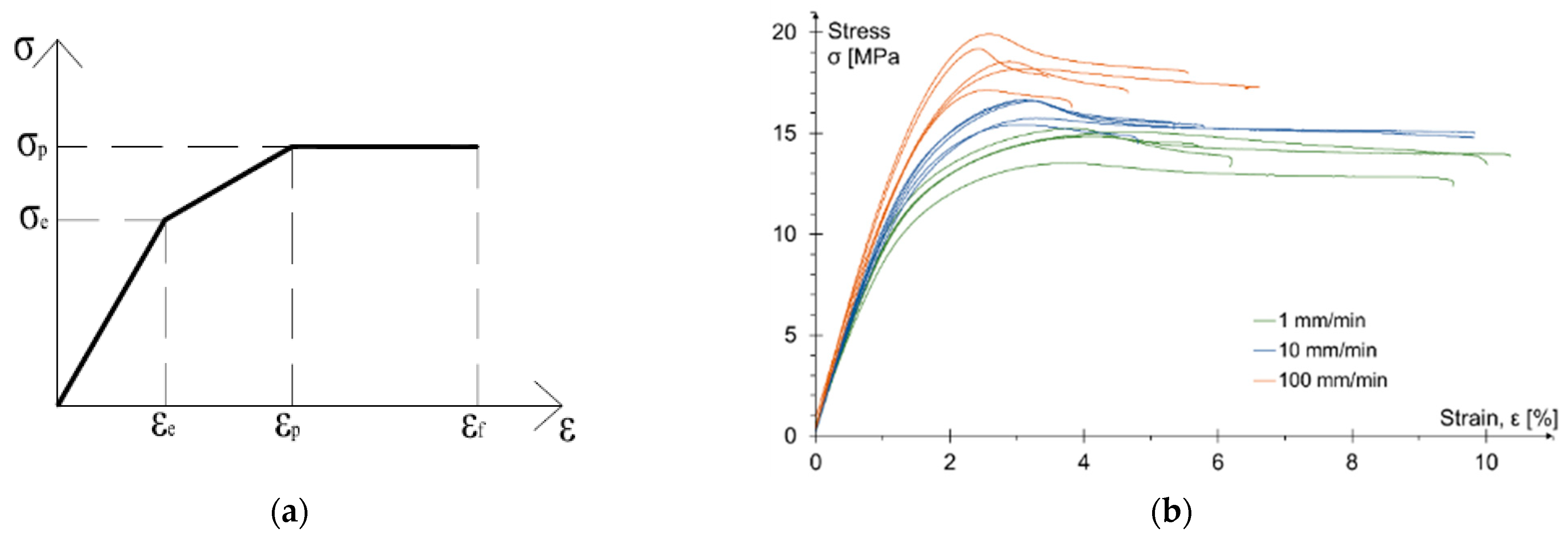
| Test Speed [mm/min] | Elastic Strength σe [MPa] | COV [%] | Elastic Strain εe [%] | COV [%] | Yield Strength σp [MPa] | COV [%] | Yield Stain εp [%] | COV [%] | Failure Strain εf [%] | COV [%] | E-modulus [MPa] | COV [%] |
|---|---|---|---|---|---|---|---|---|---|---|---|---|
| 1 | 8.0 | 7.5 | 0.8 | 25.0 | 14.7 | 4.1 | 4.1 | 7.3 | 8.4 | 23.8 | 1058 | 5.9 |
| 10 | 11.0 | 5.4 | 1.2 | 33.3 | 16.2 | 3.1 | 3.2 | 3.1 | 6.8 | 27.9 | 1131 | 2.1 |
| 100 | 13.9 | 4.3 | 1.4 | 21.4 | 18.3 | 3.8 | 2.4 | 4.1 | 4.6 | 39.1 | 1224 | 4.7 |
| Data | Test Speed [mm/Min] | Tensile Strength [MPa] | E-Modulus [MPa] | Elongation at Rapture [%] | Shear Strength [MPa] |
|---|---|---|---|---|---|
| Technical data | 50 1 | 18.6–20.6 | 517–689 | 30–50 2 | 20.7−26.2 2 (SLJ) |
| Model with 200/400 mm Overlap | Model with 400/400 mm Overlap | |||||
|---|---|---|---|---|---|---|
| A.1 | A.2 | A.3 | B.1 | B.2 | B.3 | |
| 3.10 mm | 3.35 mm | 3.63 mm | 2.31 mm | 2.95 mm | 6.00 mm | |
| Laboratory tests | ||||||
| Mean value [kN] | 299.0 | 311.2 | 319.7 | 264.1 | 323.1 | 411.2 |
| COV [%] | 1.1 | 1.4 | 2.3 | 1.1 | 1.5 | 1.3 |
| Numerical model | ||||||
| Value [kN] | 298.5 | 314.0 | 318.6 | 270.2 | 332.6 | 406.2 |
| Difference | 0.17% | 0.90% | 0.34% | 2.31% | 2.94% | 1.22% |
| Points Given in Figure 14a | |||
|---|---|---|---|
| A.1 | A.2 | A.3 | |
| Loss of adhesion: adhesive—base plate (90 × 6 mm) | 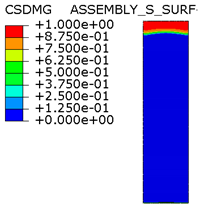 |  | 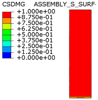 |
| The plastic phase of the adhesive layer and base plate | 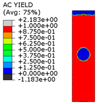 | 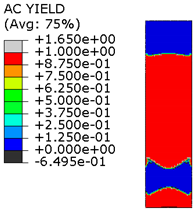 | 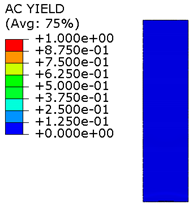 |
| Loss of adhesion: adhesive—overlap (50 × 6 mm) |  | 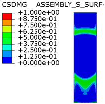 | 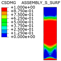 |
| Points Given in Figure 14b | |||
|---|---|---|---|
| B.1 | B.2 | B.3 | |
| The plastic phase of the adhesive layer and base plate (90 × 6 mm) | 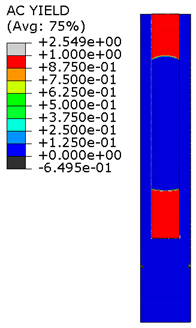 | 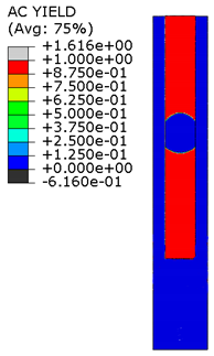 | 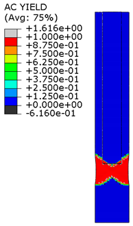 |
Publisher’s Note: MDPI stays neutral with regard to jurisdictional claims in published maps and institutional affiliations. |
© 2022 by the authors. Licensee MDPI, Basel, Switzerland. This article is an open access article distributed under the terms and conditions of the Creative Commons Attribution (CC BY) license (https://creativecommons.org/licenses/by/4.0/).
Share and Cite
Kałuża, M.; Hulimka, J.; Bula, A. FEM Analysis as a Tool to Study the Behavior of Methacrylate Adhesive in a Full-Scale Steel-Steel Shear Joint. Materials 2022, 15, 330. https://doi.org/10.3390/ma15010330
Kałuża M, Hulimka J, Bula A. FEM Analysis as a Tool to Study the Behavior of Methacrylate Adhesive in a Full-Scale Steel-Steel Shear Joint. Materials. 2022; 15(1):330. https://doi.org/10.3390/ma15010330
Chicago/Turabian StyleKałuża, Marta, Jacek Hulimka, and Arkadiusz Bula. 2022. "FEM Analysis as a Tool to Study the Behavior of Methacrylate Adhesive in a Full-Scale Steel-Steel Shear Joint" Materials 15, no. 1: 330. https://doi.org/10.3390/ma15010330
APA StyleKałuża, M., Hulimka, J., & Bula, A. (2022). FEM Analysis as a Tool to Study the Behavior of Methacrylate Adhesive in a Full-Scale Steel-Steel Shear Joint. Materials, 15(1), 330. https://doi.org/10.3390/ma15010330