Article

A Nonlinear Constitutive Model for Remoulded Fine-Grained Materials Used under the Qinghai–Tibet Railway Line

1
Railway Engineering Research Institute, China Academy of Railway Sciences Corporation Limited, Beijing 100081, China
2
School of Civil Engineering, Harbin Institute of Technology, Harbin 150090, China
3
State Key Laboratory for Geomechanics and Deep Underground Engineering, China University of Mining and Technology, Xuzhou 221008, China
4
Chongqing Research Institute, Harbin Institute of Technology, Chongqing 401135, China
*
Author to whom correspondence should be addressed.
Materials 2022, 15(15), 5119; https://doi.org/10.3390/ma15155119
Submission received: 4 June 2022 / Revised: 19 July 2022 / Accepted: 20 July 2022 / Published: 23 July 2022
(This article belongs to the Section Construction and Building Materials)

Abstract

:
Using undrained triaxial shear tests, this study investigates the mechanical properties of fine-grained materials (silty clay and sand) which are extensively used for China’s Qinghai–Tibet Railway (QTR) under different confining pressures (σ3) and freezing temperatures (T). The results show that a reduction in T causes an increase in the shear strength and elastic modulus of all the materials tested in the present study. In addition, the freezing of the silty clay has no significant effect on the type of soil behaviour (strain-hardening), whereas the freezing of the sand changes its strain-hardening behaviour to strain-softening. Supposing that the deviatoric stress–strain curves of the silty clay and sand can be divided into two segments due to a reverse bending point, it was assumed that the first segment follows a hyperbolic function. Meanwhile, the second segment is also a hyperbola, with the reverse bending point as the origin and the residual strength as the asymptote. Accordingly, a nonlinear relation constitutive model that considers σ3 and T is derived. All model parameters are identified. The reasonability of the new model was verified using the test results of the materials. A comparison of the predicted and test results shows that this model can well simulate the deviatoric stress–strain response in the failure process of the tested materials. In particular, it can reflect the residual deviatoric stress after the materials’ failure.

1. Introduction

The territory covered by frozen soil in China is the third largest in the world and includes 2.15 × 10⁶ km2 of permafrost areas [1]. Many key projects in China, such as railways, highways, and distance pipelines were built in these regions [2]. Among them, the Qinghai–Tibet Railway (QTR) is the highest and longest plateau railway in the world at present [3,4,5]. However, it has been reported that a large amount of frost damage has occurred since the QTR was built [6]. Therefore, it was essential for engineering design and maintenance to systematically investigate the mechanical properties of the frozen remoulded fine-grained materials.
In previous studies, the strength and deformation properties of frozen soil under static conditions considering different influencing factors have been researched. The influence of freezing temperatures (T) on the physical and mechanical characteristics of silty clay has been studied by many researchers [7,8,9,10,11,12,13]. It has been shown that T could significantly improve the physical and mechanical properties of soils due to the formation of a rigid ice–soil matrix [14]. Li et al. [15], Lat et al. [16], and Xu et al. [17] investigated the effects of the confining pressure (σ3), T, and moisture content on the static strength, stiffness, and damage behaviour of frozen soil by a series of triaxial static tests. However, the σ3 of previous work on frozen soil was relatively high, limited by the test equipment. Due to the low σ3 of the subgrade filling under the actual rail transit subgrade load in cold regions, the test results of a high σ3 fail to meet the engineering needs.
To master the working state of frozen soil in engineering structures, it is necessary to select the appropriate material constitutive model for analysis according to the actual situation [18]. Based on the experimental results, many constitutive models have been proposed to analytically and numerically study the strength and stress–strain relationship in frozen soil [19,20,21,22]. The Duncan–Chang constitutive model has clear concepts and is easy to understand [23,24]; so, it is widely used in hydraulic and geotechnical engineering, because it can better reflect the nonlinear behaviour of soil [25,26,27]. However, the Duncan–Chang model is not suitable for the evaluation of the frozen soil stress–strain curve, because the softening process of frozen soil cannot be well simulated.
In the following sections, the deformational characteristics of the silty clay and sand under different σ3 and T are investigated using static triaxial tests. A simplified nonlinear constitutive model that can capture strain-softening behaviour is developed to analyse the effects of σ3 and T. Next, the parameters involved in the model are evaluated, and insights and conclusions are drawn from the results.

2. Materials and Methods

2.1. Study Area and Soil Properties

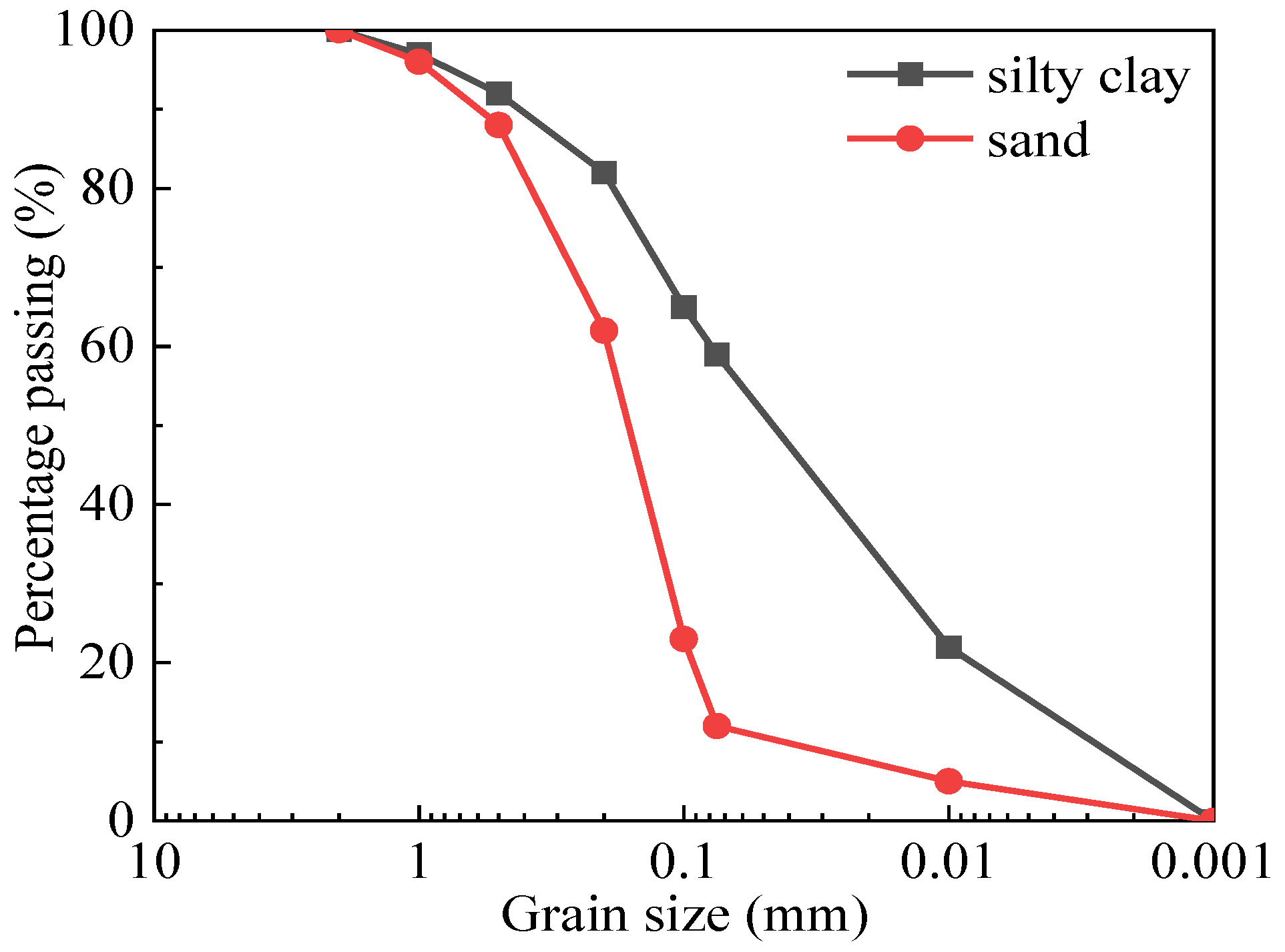
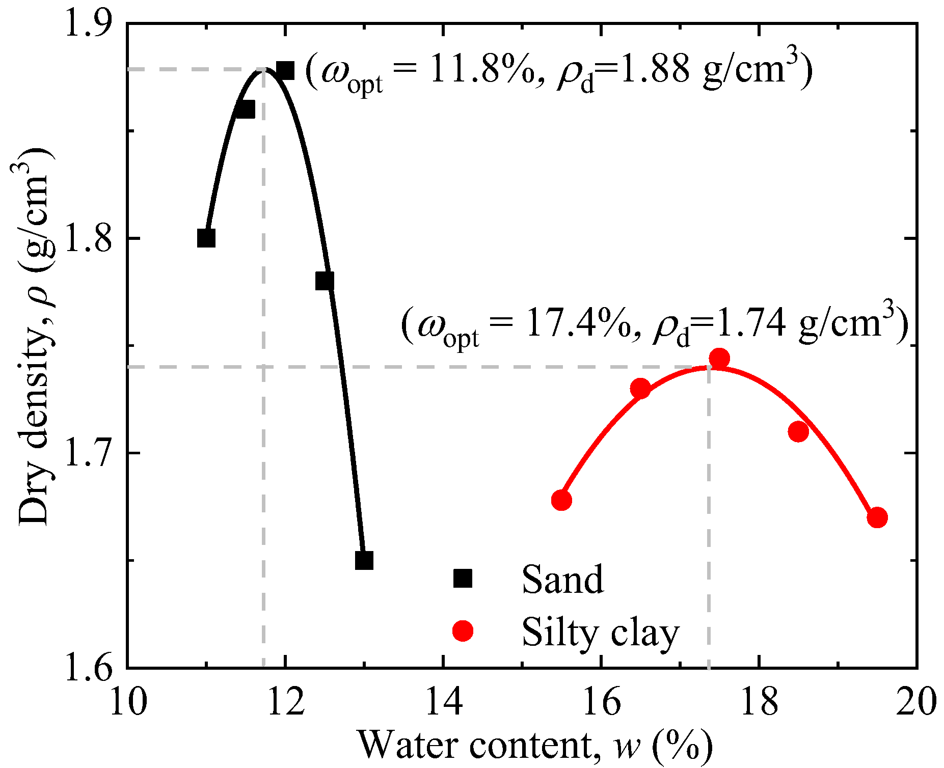
The silty clay and sand of the remoulded samples was collected within the range of 0.5 m under the shoulder at section K1013 along the Qinghai–Tibet Railway, the highest altitude railway in China’s permafrost regions (see Figure 1). The gradation curves of the soil sample are shown in Figure 2. Through laboratory tests, the optimal moisture content of the silty clay was found to be 17.4%, and the corresponding maximum dry density was 1.74 g/cm3 (see Figure 3). The optimal moisture content of the sand was 11.8%, and the corresponding maximum dry density was 1.88 g/cm3 (see Figure 3). The two fillings basically accorded with the typical characteristics of the density and optimal water content of silty clay and sand, respectively.

2.2. Sample Preparation

According to the Code for Soil Tests of Railway Engineering in China (TB10102-2010) [28], the method of sample compaction at different layers was adopted in the current study. The silty clay and sand obtained from the Qinghai–Tibet Railway was cleaned, dried, and sieved, and only the particles under a 2 mm diameter sieve were collected to make the remoulded samples. The samples were divided into five layers to compact, where the mass of each layer could be obtained considering 95% of maximum dry density (ρd, max). Subsequently, purified water was added to reach the optimum moisture content (w). Later on, the prepared soil mixtures were kept in enclosed bags for 24 h to prevent evaporation. Lastly, the cylindrical material samples with a height of 200 mm and a diameter of 100 mm were compacted layer-by-layer using a standard proctor hammer. After compacting one layer, the layer interface was made sufficiently coarse to ensure the two layers were integrated. Then, the specimens were wrapped with rubber sleeves, and the top and bottom were covered with epoxy resin platen to prevent water evaporation.

2.3. Test Procedures

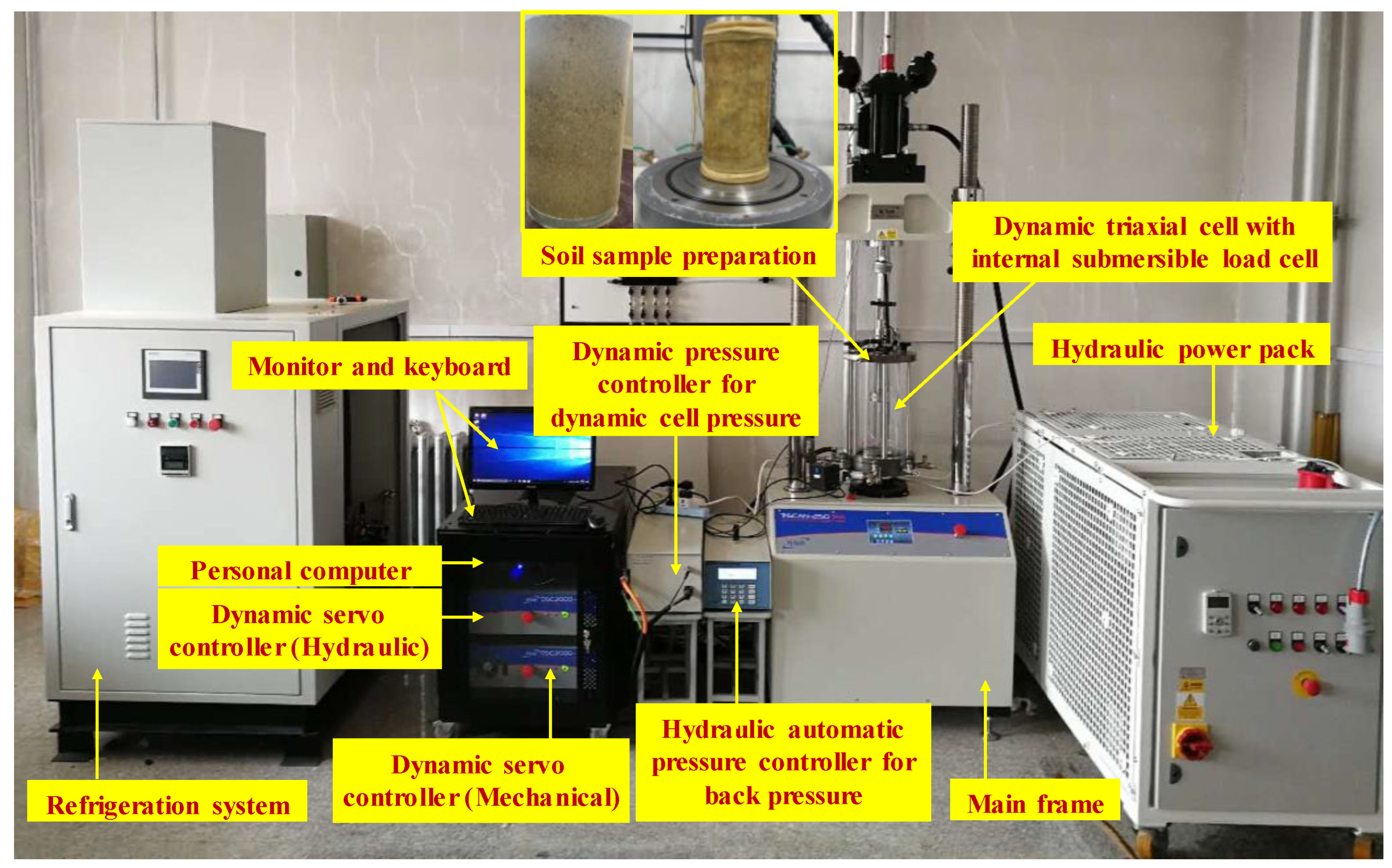
The dynamic triaxial tests were conducted on a fully automated Global Digital System (GDS), a cryogenic triaxial apparatus, illustrated in Figure 4. The system is a digitally controlled servo pneumatic system that controls two parameters: axial stress and confining pressure (σ3). The system incorporated a control and data acquisition system, which can maintain an auxiliary air receiver with a servo valve for cell pressure control, local deformation measurement in the vertical direction, and a submersible load cell measuring the applied axial load. The stable confining pressure ranged from 20 kPa to 4 MPa, and the maximum axial load and displacement were 40 kN and 85 mm, respectively.
According to Wang et al. [29], a closed system was adopted for the test program. A one-dimensional freezing–thawing model was employed to simulate the direction of freezing and thawing from the top to the bottom. To ensure one-dimensional freezing and thawing, only the sample top surface was exposed to the external environment. A 50 mm thick layer of insulating polystyrene was used to protect the perimeter and bottom of the cylinder.
The variation range in ground temperature along the Qinghai–Tibet Railway in China is roughly between −20 °C and 20 °C, with a large temperature difference. Therefore, the temperatures under the static loading condition were set to −10 °C, −5 °C, and −1 °C. The time needed to freeze the sample was determined by a pre-experiment test. A short resistance temperature detector probe was inserted at the centre of a pre-experiment test sample during the freezing process to show the variation in temperature. It revealed that 12 h was sufficient to freeze the sample to reach −10 °C with slight fluctuations, plus or minus 0.2 °C.
The test sample was isotropically consolidated at σ3 = 100 kPa, 150 kPa, or 200 kPa after the sample temperature was under the preset temperature for 12 h. After consolidation, the test specimen was then subjected to shearing at an axial strain rate (1.25 mm per min) until the strain of 15% was reached. The particular test scheme is shown in Table 1.

3. Experiment Results and Analysis

3.1. Stress–Strain Behaviour

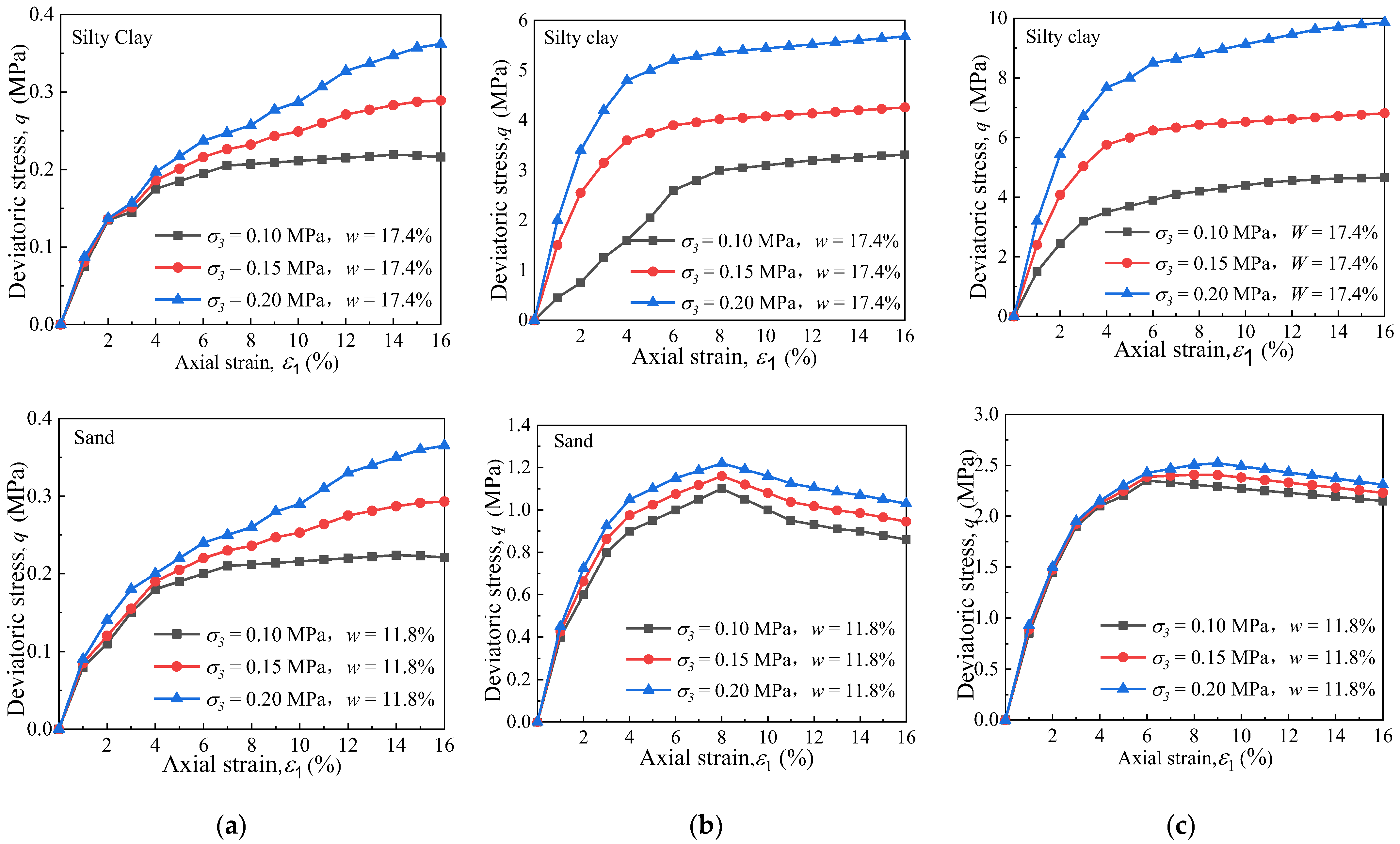
To illustrate the mechanical behaviour of the remoulded fine-grained materials that were influenced by the freezing temperature and σ3, Figure 5 shows the typical stress–strain curves for the samples. The results show that the shear strength of the frozen silty clay was significantly greater than that of the frozen sand at the same conditions, especially at low temperatures. It is seen that all the stress–strain curves for silty clay were of the strain-hardening type, and the principal stress deviation had nonlinear growth with the increase in the axial strain, in which the shape of curves was hyperbolic. The stress–strain curves of the silty clay show that the shape of the stress–strain curve did not change with the variation in the temperature, but the degree of hardening was weakened. Decreasing the freezing temperature to −5 °C and −10 °C increased the shear strength of the silty clay by 1374% and 2258% with respect to the silty clay of −1 °C when the σ3 = 150 kPa.
As for the sand, when the freezing temperature was the same, the stress–strain curves’ variation tendency was similar with the different σ3. However, the stress–strain curves gradually changed to strain-softening as the freezing temperature decreased. Moreover, the reduction in the temperature from −1 °C to −10 °C caused an increase in the shear strength of 661% for the frozen sand under a σ3 of 150 kPa. It can be concluded that the influence of freezing on the increase in shear strength of the silty clay was much greater than that for sand.

3.2. Cohesion and Internal Friction Angle

The results in Figure 5 were processed using the Mohr–Coulomb strength criterion expressed by the “p-q” method to obtain the internal friction angle φ and cohesion c in Figure 6. According to Figure 6, the samples of silty clay with more water content than that of sand strengthened the bite friction during the freezing process; so, the cohesion and angle of the internal friction in silty clay were slightly greater than those in sand. Here, the cohesion increased by approximately 5900% and 3100% for silty clay and sand, respectively, comparing the samples at the temperatures of −1 °C and −10 °C. Similar to the cohesion, the reduction in temperature from −1 °C to −10 °C led to an 11.1% and 8.4% increase in the internal friction angle of silty clay and sand, respectively. It is noted that the rate of increase in the cohesion and angle of internal friction due to the reduction in temperature was almost identical for the silty clay and sand.

3.3. Elastic Modulus

The effect of σ3 and freezing temperature reduction on the modulus of elasticity (Ee) of the silty clay is presented in Figure 7a. The values of Ee for the silty clay under the temperature of −1 °C for σ3 values of 100, 150, and 200 kPa were approximately 7.5, 9, and 10 MPa, respectively. After the freezing temperature decreased to −5 °C, the growth in Ee was approximately 900%, 1567%, and 1880%, respectively. As the freezing temperature continued to decrease to −10 °C, the values of Ee increased by 1793%, 1844%, and 2230% with respect to the silty clay at −1 °C for the three σ3 values, respectively.
Moreover, a decrease in freezing temperature led to a significant increase in the Ee of sand. Figure 7b presents the effect of the freezing temperature reduction on the Ee of the sand tested under σ3 values of 100, 150, and 200 kPa at the freezing temperature of −10 °C, −5 °C, and −1 °C. As expected, the Ee of sand generally increased with the decreasing freezing temperature. The growth in the Ee of sand under the freezing temperature of −10 °C relative to the sand at −1 °C was approximately 775%, 743%, and 715%, respectively, for the three σ3 values.

4. A Nonlinear Constitutive Model for Remoulded Fine-Grained Materials

4.1. Establishment of the Model

As shown in Figure 8, a softening-type stress–strain model with a high degree of accuracy can be used to approximate the nonlinear stress–strain curves for the remoulded fine-grained materials under different freezing temperatures [30]. After careful inspection, the piecewise continuous functions for the proposed constitutive model are expressed as follows:
R σ = D β 1 + b 2 R ε 1 + b 3 R ε R ε 1 + b 1 R ε R ε R ε t        
R σ = R σ t R ε R ε t b 4 + b 5 R ε R ε t                                             R ε > R ε t    
where Dβ, b1, b2, b3, b4, and b5 are undetermined coefficients that can be obtained from the experimental results. The parameters Rσ, Rε, Rσt, and Rεt are defined by Equation (2a) through (2d) as follows:
R σ = σ 1 σ 3 σ 1 σ 3 p
R ε = ε ε p
R σ t = σ 1 σ 3 t σ 1 σ 3 p
R ε t = ε t ε p
where (σ1σ3) is the deviator stress; σ1 and σ3 are the major principal stress and minor principal stress, respectively; ε is the axial strain; (σ1σ3)p and εp are the deviator stress and deviator strain, respectively, at the peak point (i.e., point P in Figure 8); and (σ1σ3)t and εp are the deviator stress and the deviator strain, respectively, at the inflection point (i.e., point T in Figure 8).
(1)
Coefficient determination for Equation (1a).
To accurately represent the relationship between (σ1σ3) and Rε, the terms on both sides of Equation (1a) were multiplied by (σ1σ3)p and Equation (1a) was rewritten as follows:
σ 1 σ 3 = D β σ 1 σ 3 p 1 + b 2 R ε 1 + b 3 R ε R ε 1 + b 1 R ε
The compressive strengths of the fillers are assumed to satisfy the Mohr–Coulomb failure criterion. The relationship between the compressive strength (σ1σ3)p and the confining pressure σ3 is described by the following equation:
σ 1 σ 3 p = 2 c p cos φ p + σ 3 sin φ p 1 sin φ p
in which cp and φp are the Mohr–Coulomb strength parameters.
Next, Equation (4) is substituted for (σ1σ3)p in Equation (3) to yield
σ 1 σ 3 = D β 2 C p cos φ p + σ 3 sin φ p 1 sin φ p 1 + b 2 R ε 1 + b 3 R ε R ε 1 + b 1 R ε
where Dβ = D × β, with β as a modified coefficient and D = Emax/Ep. Emax and Ep (i.e., Ep = (σ1σ3)p/εp) are the initial tangent modulus at the original point (i.e., point O in Figure 8) and the secant modulus at the peak point, respectively. The determination of Emax is equivalent to the determination of Emax in the Duncan–Chang model [23].
Performing the differentiation on Equation (1a) produces the following expression
d R σ d R ε = D β 1 1 + b 1 R ε 1 + b 3 R ε b 1 b 2 R ε 1 + b 3 R ε + 1 + b 2 R ε 1 + b 1 R ε
In addition, Rσ can be considered as a function of the parameter Rε in Equation (1a) and attains its extreme value at the peak. Thus,
d R σ d R ε = 0
Combined with Equations (6) and (7),
b 1 b 2 1 + b 3 + 1 + b 2 1 + b 1 = 0
b 1 = b 2 b 3 + 2 b 2 + 1 b 3 b 2
In this case, Rσ = 1 and Rε = 1 at the peak point based on their definitions in Equation (2). Thus, these values are substituted into Equation (1a) to obtain
1 = D β 1 + b 2 1 + b 3 1 1 + b 1
According to Equation (1a), Rεt and Rσt may be expressed at the inflection point as follows:
R σ t = D β 1 + b 2 R ε t 1 + b 3 R ε t 1 1 + b 1 R ε t
By combining Equations (9) and (10), b2 and b3 can be expressed as
b 3 = R ε t 1 + β t 1 + b 1 R ε t β p 1 + b 1 R ε t β p 1 + b 1 R ε t β t 1 + b 1 R ε t R ε t
b 2 = β p 1 + b 1 1 + b 3 1
where β t = R σ t D β R ε t and β p = R σ p D β R ε p .
Three undetermined coefficients (i.e., b1, b2, and b3) are included in Equation (11). When the original b1 is given, b2 and b3 are evaluated using Equations (11a) and (11b). Subsequently, b2 and b3 are substituted into Equation (8) to obtain a new value for b1. This procedure can be repeated by using the original b1 until the given and recalculated b1 are identical.
(2)
Coefficients of determination for Equation (1b).
Similarly, the terms on both sides of Equation (1b) are simultaneously multiplied by (σ1σ3)p. Next, Equation (1b) is combined with Equation (2a) to (2d) as follows:
σ 1 σ 3 = σ 1 σ 3 t ε ε t 1 E p b 4 + 1 E p ε p b 5 ε ε t
If we let
b4 = EpA
b5 = EpεpB
then, Equation (12) is rewritten as
σ 1 σ 3 = σ 1 σ 3 t ε ε t A + B ε ε t
The tangent modulus (E) at any point in the first segment of the curve (i.e., RεRεt) can be directly represented as
E = d σ 1 σ 3 d ε = d σ 1 σ 3 d R σ d R σ d R ε d R ε d ε
The expressions of Rσ and Rε can be rewritten as
d σ 1 σ 3 d R σ = σ 1 σ 3 p
d R ε d ε = 1 ε p
Equation (16) is substituted into Equation (15) to obtain
d σ 1 σ 3 d ε = σ 1 σ 3 p ε σ d R σ d R ε = E p d R σ d R ε
Equation (6) is substituted into Equation (17), and the tangent modulus in the first segment of the curve can be expressed as
d σ 1 σ 3 d ε = D β E p 1 + b 1 R ε 1 + b 3 R ε b 1 b 2 R ε 1 + b 3 R ε + 1 + b 2 R ε 1 + b 1 R ε
In addition, Dβ = D × β, D = Emax/Ep, Equation (18) can be rewritten as
d σ 1 σ 3 d ε = E max 1 + b 1 R ε 1 + b 3 R ε b 1 b 2 R ε 1 + b 3 R ε + 1 + b 2 R ε 1 + b 1 R ε
Therefore, the tangent modulus ( E ¯ t , 1 ) at the inflection point in the first segment of the curve can be obtained from Equation (19).
E ¯ t , 1 = E max 1 + b 1 R ε t 1 + b 3 R ε t b 1 b 2 R ε t 1 + b 3 R ε t + 1 + b 2 R ε t 1 + b 1 R ε t
In addition, the tangent modulus ( E ¯ t , 2 ) at the inflection point in the second segment of the curve can be expressed from Equation (12) by using Equation (21) in terms of the definition of the derivative.
E ¯ t , 2 = lim ε ε t σ 1 σ 3 σ 1 σ 3 t ε ε t = lim ε ε t 1 A + B ε ε t = 1 A
To ensure a continuous condition at the inflection point, the tangent modulus at the inflection point in the two segments of the curve should be equivalent, which indicates that E ¯ t , 1 = E ¯ t , 2 at the inflection point. Therefore, Equation (21) is substituted into Equation (20) to obtain
A = 1 E max 1 + b 1 R ε t 1 + b 3 R ε t b 1 b 2 R ε t 1 + b 3 R ε t + 1 + b 2 R ε t 1 + b 1 R ε t
Consequently, b4 can be evaluated when the value of A is substituted into Equation (13a).
When the deviatoric stress (σ1σ3)r, which is the residual strength and its corresponding strain εr at any point in the second segment of the curve, is substituted into Equation (2), Rσr and Rεr can be evaluated, and b5 can be obtained using Equation (23). In this study, the residual deviatoric stress (σ1σ3)r is selected when the strain εr is equivalent to 20%.
b 5 = b 4 + R ε r R ε t R σ r R σ t R ε r R ε t

4.2. Determination of Model Parameters

Six parameters need to be determined from Equation (1) in the proposed model, including the parameters related to the basic elastic properties (Dβ), the peak stress state (b1, b2, and b3), and the residual stress state (b4 and b5). Most of these model parameters can be conveniently obtained through the monotonic triaxial tests incorporating σ3 and T. The initial small stress–strain data can be adopted to calculate the Dβ. The residual stress state parameters (b4 and b5) can be evaluated through the monotonic triaxial tests results at the residual stress state using Equations (13) and (23). The peak state parameters (b1, b2, and b3) can be determined by a trial-and-error process using Equations (8) and (11), i.e., by comparing the model predictions and laboratory data. Furthermore, the values of the abovementioned undetermined coefficients with the corresponding values are shown in Table 1.

4.3. Model Verification

The test results of the sand and silty clay subjected to different σ3 and T are used to validate the proposed model. Figure 9 shows the predicted stress–strain of the sand and silty clay compared to the laboratory observations. Note that the model predictions match well with the test data, and the strain-hardening and strain-softening of the samples subjected to different σ3 and T have been captured very well.

5. Discussion

5.1. Sensitivity Analysis of the Parameters

In Equation (1a), let b1 = 0.78, b2 = −0.44, and b3 = 0.21; thus, Figure 10a demonstrates the deviatoric stress–strain curves of the proposed constitutive model for different values of the parameter Dβ. It can be seen from Figure 10a that the change in the value Dβ has no obvious influence on the shape of the deviatoric stress–strain curve. However, with the increase in the value Dβ, the initial elastic modulus of the model increases gradually, indicating that the parameter Dβ mainly reflects the initial elastic modulus of the materials; indeed, the larger the parameter Dβ is, the higher the initial elastic modulus will be.
Furthermore, in Equation (1a), let Dβ = 3.86, b2 = −0.44, and b3 = 0.21; let Dβ = 3.86, b1 = 0.78, and b3 = 0.21; and let Dβ = 3.86, b1 = 0.78, and b2 = −0.44; Thus, Figure 10b,d presents the deviatoric stress–strain curves of the proposed constitutive model for different values of the parameters b1, b2, and b3, respectively. Figure 10b,d show that the change in the values b1, b2, and b3 has a great influence on the shape of the deviatoric stress–strain curve. With a decrease in the values b1 and b3 and an increase in the value b2, the stress–strain curves gradually change from strain-softening to strain-hardening. This indicates that the parameters b1, b2, and b3 mainly reflect the peak strength and brittleness degree of the materials’ failure. The larger the parameters b1 and b3 are, and the smaller the parameter b2 is, the more obvious the brittleness failure characteristic of the materials will be.
In addition, it can be seen from Figure 10 that the variation in b4 and b5 only changes the shape of the residual stress state. With an increase in b4 and b5, the residual stress increases, indicating that the failure characteristic changes from brittleness to ductility.

5.2. Comparison with the Existing Model

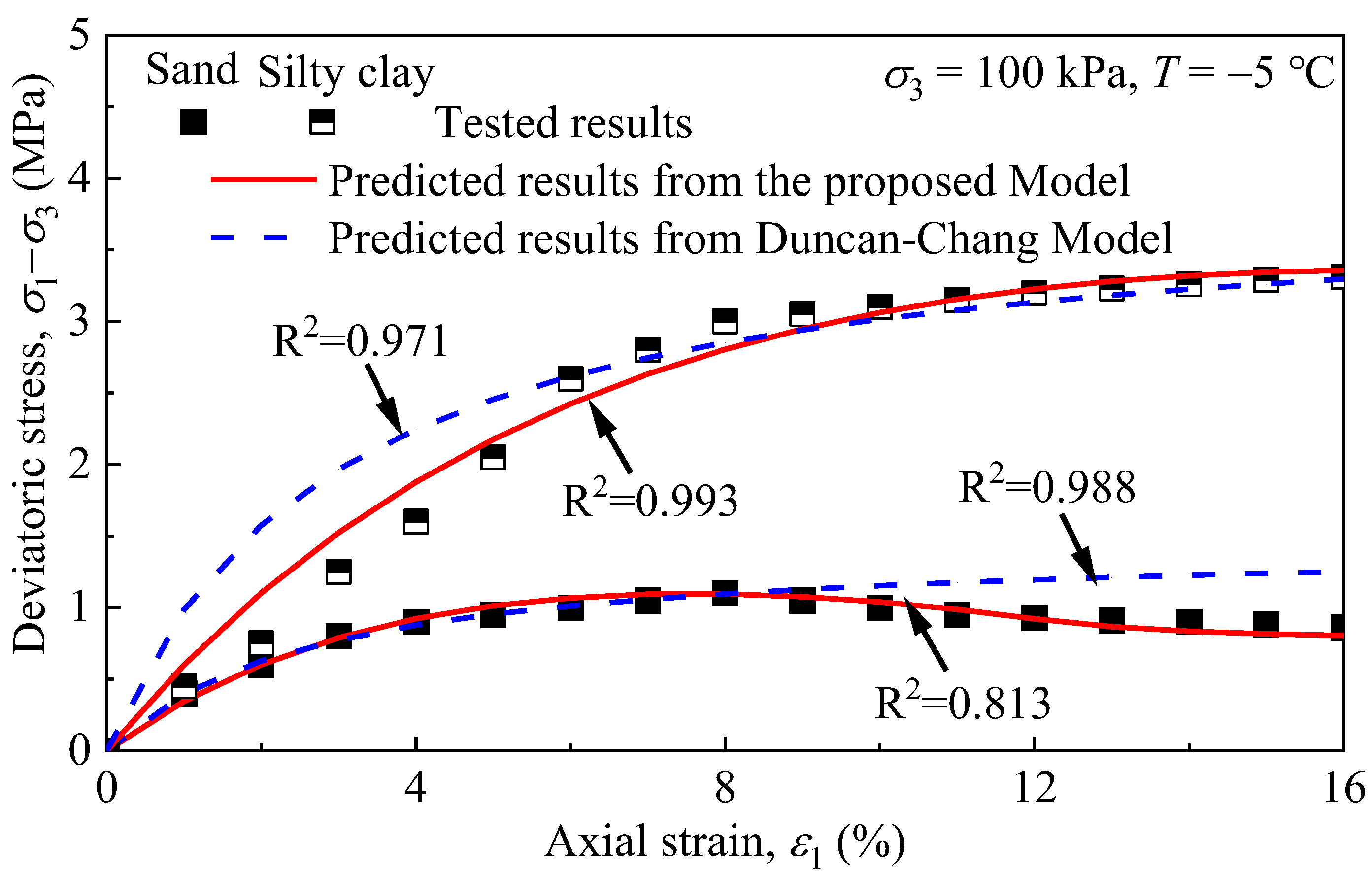
In order to further illustrate the rationality of the proposed model, the triaxial compression test results of silty clay and sand, with σ3 = 100 kPa and T = −5 °C, were employed to validate it. Figure 11 presents the comparison of the theoretical curves from the proposed model and the Duncan–Chang model. It can be seen from Figure 11 that the theoretical curves from the Duncan–Chang model had good agreement with the test data at the prepeak region but poor agreement at the postpeak region for the mechanical behaviours of the materials. In particular, it could not reflect the residual deviatoric stress after the materials’ failure, while the theoretical curves from the model proposed in the current study conform well with the test data in both the prepeak region and postpeak region, no matter what the shape of the stress–strain curves. Therefore, the proposed model has better adaptability.

6. Conclusions

This paper presented the results of a comprehensive experimental investigation to study the effect of confining pressure (σ3) and freezing temperature (T) on the mechanical behaviour of remoulded fine-grained materials (silty clay and sand) used under the Qinghai–Tibet Railway line. Accordingly, a nonlinear constitutive model, which could reflect the postpeak softening behaviour was established. Conventional monotonic triaxial tests incorporating σ3 and T carried out in the current study were used to evaluate all the model parameters. The salient outcomes of the model are summarized below.
(1)
All the silty clay exhibited a strain-hardening type of stress–strain curve, but the sand under the temperatures of −5 °C and −10 °C showed strain-softening. Under the same test conditions, the shear strength of the silty clay was greater than that of the sand. In all cases, the cohesion (c) and angle of internal friction (φ) of the silty clay were greater than that of sand. Furthermore, the modulus of elasticity of the materials tested increased due to freezing and the temperature reduction.
(2)
A practical constitutive model was developed to represent the nonlinear, stress-dependent, and inelastic stress–strain behaviours of the fillers subjected to freezing and thawing. This model incorporated three important aspects of the stress–strain behaviour, including nonlinearity, strain-dependency softening, and inelasticity. A simple technique was used to interpret the test results and conveniently determine the six parameters in the model.
(3)
The triaxial test results of the remoulded fine-grained materials were employed to evaluate the reasonability of the proposed model established in this paper. A comparison of the predicted and test results showed that this model could well simulate the deviatoric stress–strain response in the failure process of the tested materials. In particular, it could reflect the residual deviatoric stress after materials’ failure.
(4)
This study analysed the behaviour of the fillers with optimum water content that were exposed to the freeze–thaw cycles to develop a constitutive model. If appropriate experimental results are available, the parameter values in the proposed model can be derived from the triaxial test results. Therefore, additional experiments should be conducted to investigate other parameters, such as the temperature, duration of freezing and thawing, and the moisture content and compactness of the fillers, which are important characteristics of fillers in regions that are subjected to seasonal freezing and thawing.

Author Contributions

Conceptualization and methodology, S.T.; validation, K.W. and X.H.; writing—original draft preparation, L.D. and C.Y.; writing—review and editing, S.T. and C.Y.; funding acquisition, L.D. All authors have read and agreed to the published version of the manuscript.

Funding

This research was funded by the Major Program of China Academy of Railway Sciences (grant no. 2020YJ037, Project Leader: Liang Dong) and the National Natural Science Foundation of China (grant no. 42072316 and 42102311, Project Leader: Liang Dong and Shuang Tian, respectively).

Institutional Review Board Statement

Not applicable.

Informed Consent Statement

Not applicable.

Data Availability Statement

Not applicable.

Conflicts of Interest

The authors declare no conflict of interest.

References

  1. Zhao, F.T.; Chang, L.J.; Zhang, W.Y. Experimental investigation of dynamic shear modulus and damping ratio of Qinghai-Tibet frozen silt under multi-stage cyclic loading. Cold Reg. Sci. Technol. 2020, 170, 102938. [Google Scholar] [CrossRef]
  2. Ma, D.D.; Ma, Q.Y.; Yao, Z.M.; Huang, K. Static-dynamic coupling mechanical properties and constitutive model of artificial frozen silty clay under triaxial compression. Cold Reg. Sci. Technol. 2019, 167, 102858. [Google Scholar] [CrossRef]
  3. Wu, Q.B.; Cheng, G.D.; Ma, W.; Niu, F.J.; Sun, Z.Z. Technical approaches on permafrost thermal stability for Qinghai–Xizang Railroad. Geomech. Geoeng. 2006, 1, 119–128. [Google Scholar] [CrossRef]
  4. Ma, W.; Cheng, G.D.; Wu, Q.B.; Wang, D.Y. Application on idea of dynamic design in Qinghai–Tibet Railway construction. Cold Reg. Sci. Technol. 2004, 41, 165–173. [Google Scholar] [CrossRef]
  5. Zu, Z.Y.; Ling, X.Z.; Chen, S.P.; Zhang, F.; Wang, L.N.; Wang, Z.Y.; Zou, Z.Y. Experimental investigation on the train-induced subsidence prediction model of Beiluhe permafrost subgrade along the Qinghai–Tibet Railway in China. Cold Reg. Sci. Technol. 2010, 62, 67–75. [Google Scholar] [CrossRef]
  6. Cheng, G.D. A roadbed cooling approach for the construction of Qinghai–Tibet Railway. Cold Reg. Sci. Technol. 2005, 42, 169–176. [Google Scholar] [CrossRef]
  7. Wang, C.; Li, S.; Zhang, T.; You, Z. Experimental Study on Mechanical Characteristics and Fracture Patterns of Unfrozen/Freezing Saturated Coal and Sandstone. Materials 2019, 12, 992. [Google Scholar] [CrossRef] [Green Version]
  8. Sobczyk, K.; Chmielewski, R.; Kruszka, L.; Rekucki, R. Strength Characterization of Soils’ Properties at High Strain Rates Using the Hopkinson Technique—A Review of Experimental Testing. Materials 2022, 15, 274. [Google Scholar] [CrossRef]
  9. Wei, X.; Ming, F.; Li, D.; Chen, L.; Liu, Y. Influence of Water Content on Mechanical Strength and Microstructure of Alkali-Activated Fly Ash/GGBFS Mortars Cured at Cold and Polar Regions. Materials 2020, 13, 138. [Google Scholar] [CrossRef] [Green Version]
  10. Zhao, X.; Zhou, G.; Wang, J. Deformation and strength behaviors of frozen clay with thermal gradient under uniaxial compression. Tunn. Undergr. Space Technol. 2013, 38, 550–558. [Google Scholar] [CrossRef]
  11. Li, H.; Yang, Z.J.; Wang, J. Unfrozen water content of permafrost during thawing by the capacitance technique. Cold Reg. Sci. Technol. 2018, 152, 15–22. [Google Scholar] [CrossRef]
  12. Török, Á.; Ficsor, A.; Davarpanah, M.; Vásárhelyi, B. Comparison of mechanical properties of dry, saturated and frozen porous rocks. In Proceedings of the IAEG/AEG Annual Meeting, San Francisco, CA, USA, 17–21 September 2018; Shakoor, A., Cato, K., Eds.; Springer International Publishing: New York, NY, USA, 2018; Volume 6, pp. 113–118. [Google Scholar]
  13. Esmaeili-Falak, M.; Katebi, H.; Javadi, A.A. Effect of Freezing on Stress–Strain Characteristics of Granular and Cohesive Soils. J. Cold Reg. Eng. 2020, 34, 05020001. [Google Scholar] [CrossRef]
  14. Wang, D.Y.; Zhu, Y.L.; Ma, W.; Niu, Y.H. Application of ultrasonic technology for physical–mechanical properties of frozen soils. Cold Reg. Sci. Technol. 2006, 44, 12–19. [Google Scholar] [CrossRef]
  15. Li, D.W.; Yang, X.; Chen, J.H. A study of Triaxial creep test and yield criterion of artificial frozen soil under unloading stress paths. Cold Reg. Sci. Technol. 2017, 141, 163–170. [Google Scholar] [CrossRef]
  16. Lai, Y.M.; Liao, M.K.; Hu, K. A constitutive model of frozen saline sandy soil based on energy dissipation theory. Int. J. Plast. 2016, 78, 84–113. [Google Scholar] [CrossRef] [Green Version]
  17. Xu, X.T.; Li, Q.L.; Lai, Y.; Pang, W.T.; Zhang, R.P. Effect of moisture content on mechanical and damage behavior of frozen loess under triaxial condition along with different confining pressures. Cold Reg. Sci. Technol. 2019, 157, 110–118. [Google Scholar] [CrossRef]
  18. Peng, W.; Wang, Q.; Liu, Y.F.; Sun, X.H.; Chen, Y.T.; Han, M.X. The Influence of Freeze-Thaw Cycles on the Mechanical Properties and Parameters of the Duncan-Chang Constitutive Model of Remolded Saline Soil in Nong’an County, Jilin Province, Northeastern China. Appl. Sci. 2019, 9, 4941. [Google Scholar] [CrossRef] [Green Version]
  19. Li, Z.; Chen, J.; Mao, C. Experimental and Theoretical Investigations of the Constitutive Relations of Artificial Frozen Silty Clay. Materials 2019, 12, 3159. [Google Scholar] [CrossRef] [Green Version]
  20. Zhang, Y.; Chen, Y. A Constitutive Relationship for Gravelly Soil Considering Fine Particle Suffusion. Materials 2017, 10, 1217. [Google Scholar] [CrossRef] [Green Version]
  21. Xu, P.; Sun, Z.; Shao, S.; Fang, L. Comparative Analysis of Common Strength Criteria of Soil Materials. Materials 2021, 14, 4302. [Google Scholar] [CrossRef]
  22. Fu, T.T.; Zhu, Z.W.; Zhang, D.; Liu, Z.J.; Xie, Q.J. Research on damage viscoelastic dynamic constitutive model of frozen soil. Cold Reg. Sci. Technol. 2019, 160, 209–221. [Google Scholar] [CrossRef]
  23. Duncan, J.M.; Chang, C.Y. Nonlinear analysis of stress and strain in soils. J. Soil Mech. Found Div. ASCE 1970, 96, 1629–1653. [Google Scholar] [CrossRef]
  24. Duncan, J.M. Strength Stress-Strain and Bulk Modulus Parameters for Finite Element Analysis of Stresses and Movements in Soil Masses; VCB/GT/78-02; University of California, Berkeley: Berkeley, CA, USA, 1978.
  25. Liu, X.Q.; Liu, J.K.; Tian, Y.H.; Chang, D.; Hu, T.F. Influence of the Freeze-thaw Effect on the Duncan-Chang Model Parameter for Lean Clay. Transp. Geotech. 2019, 21, 100273. [Google Scholar] [CrossRef]
  26. Hu, T.F.; Liu, J.K.; Chang, D.; Fang, J.H.; Xu, A.H. Influence of Freeze-thaw Cycling on Mechanical Properties of Silty Clay and Ducan-Chang Constitutive Model. Zhongguo Gonglu Xuebao/China J. Highw. Transp. 2018, 31, 298–307. [Google Scholar]
  27. He, Y.; Chen, X. The Application of Improved Duncan-Chang Model in Unloading Soil. Open Civ. Eng. J. 2014, 8, 410–415. [Google Scholar] [CrossRef] [Green Version]
  28. TB10102-2010; Code for Soil Test of Railway Engineering. China Railway First Survey and Design Institute Group: Beijing, China, 2010. (In Chinese)
  29. Wang, D.; Ma, W.; Niu, Y.; Chang, X.; Wen, Z. Effects of cyclic freezing and thawing on mechanical properties of Qinghai–Tibet clay. Cold Reg. Sci. Technol. 2007, 48, 34–43. [Google Scholar] [CrossRef]
  30. Yu, C.Y.; Tian, S.; Tang, L.; Ling, X.Z.; Zhou, G.Q. Finite element analysis on deformation of high embankment in heavy-haul railway subjected to freeze-thaw cycles. Sci. Cold Arid Reg. 2015, 7, 421–429. [Google Scholar] [CrossRef]
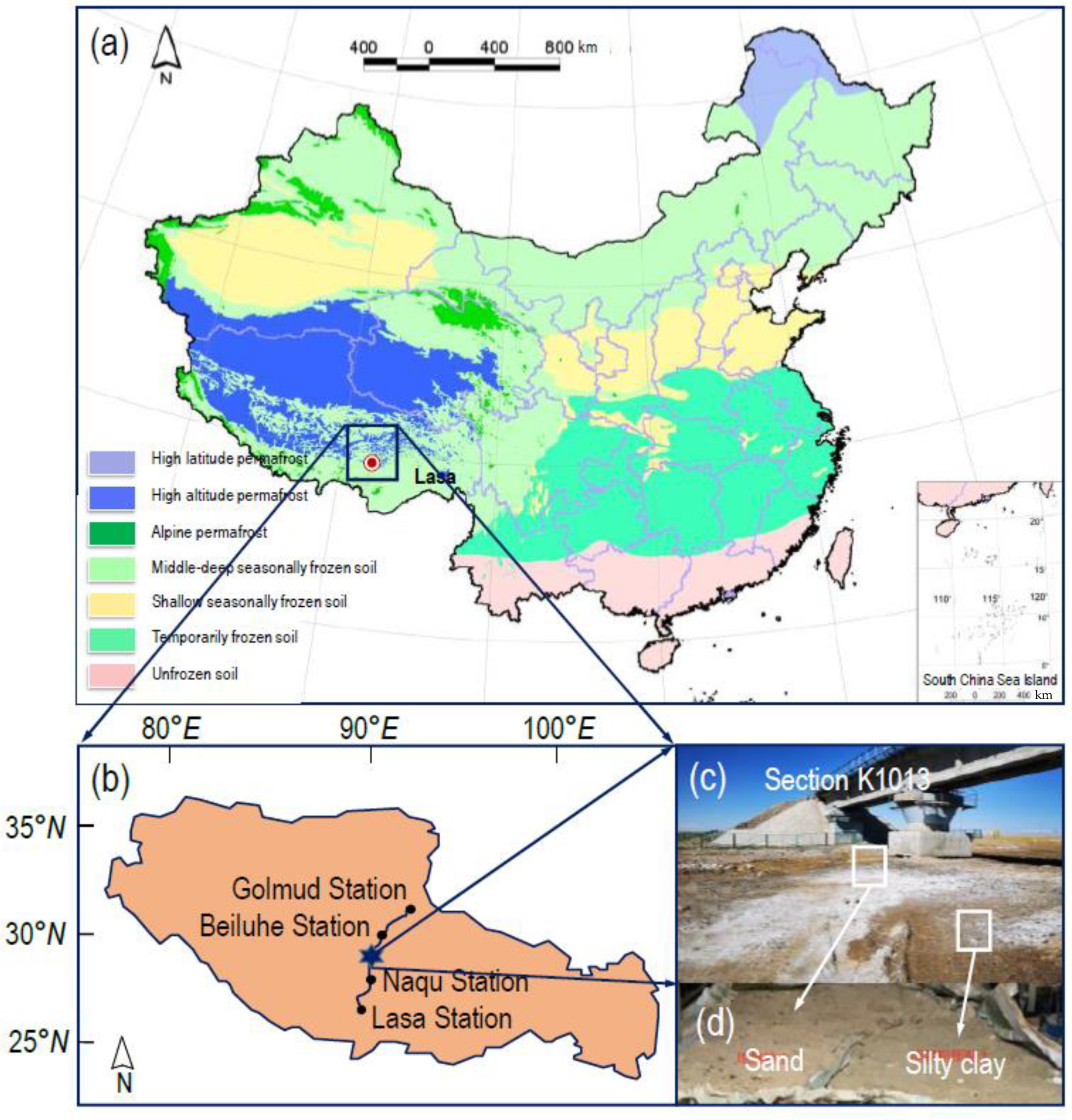
Figure 1. Remoulded fine-grained materials from Section K1013 along the Qinghai−Tibet railway: (a) frozen soil map of China; (b) Qinghai−Tibet railway; (c) section K1013 site; (d) remoulded fine-grained materials.
Materials 15 05119 g001
Figure 2. Particle size distribution curves of the remoulded fine-grained materials (silty clay and sand).
Materials 15 05119 g002
Figure 3. Compaction curve of the remoulded fine-grained materials (silty clay and sand) used in this study.
Materials 15 05119 g003
Figure 4. Cryogenic triaxial test system and the tested samples.
Materials 15 05119 g004
Figure 5. Dependence of deviatoric stress on the axial strain of tested remoulded fine-grained materials corresponding to different confining pressures: (a) T = −1 °C, (b) T = −5 °C, and (c) T = −10 °C.
Materials 15 05119 g005
Figure 6. Variation in the cohesion and angle of internal friction versus freezing temperature.
Materials 15 05119 g006
Figure 7. Variation in the elastic modulus versus freezing temperature and confining pressure: (a) silty clay and (b) sand.
Materials 15 05119 g007
Figure 8. Schematic diagram of a nonlinear constitutive model for the remoulded fine-grained materials.
Materials 15 05119 g008
Figure 9. Comparison of the predicted and tested data of the tested remoulded fine-grained materials: (a) sand and (b) silty clay.
Materials 15 05119 g009
Figure 10. Deviatoric stress–strain curves of the proposed model for different values of parameters: (a) Dβ, (b) b1, (c) b2, (d) b3, (e) b4, and (f) b5.
Materials 15 05119 g010
Figure 11. Comparison of the predicted and tested data of the tested remoulded fine-grained materials under T = −5 °C and σ3 = 100 kPa.
Materials 15 05119 g011
Table 1. Summary of test schemes and the corresponding model parameters.
Soil TypeTest No.Confining Pressure (kPa)Temperature (°C)b1b2b3b4b5DβThe Patterns of the Stress–Strain Curves
SandS1100−10.780.440.213--3.86Strain-hardening
S21500.540.460.165--3.30Strain-hardening
S32000.390.430.174--2.84Strain-hardening
S4100−50.780.380.00361.415.932.91Strain-softening
S51500.540.250.00771.226.392.53Strain-softening
S62000.390.330.00571.166.712.24Strain-softening
S7100−100.780.250.01423.6511.952.41Strain-softening
S81500.540.330.01922.609.432.35Strain-softening
S92000.390.390.04461.838.442.40Strain-softening
Silty claySC1100−11.260.420.19--4.67Strain-hardening
SC21503.730.290.24--4.94Strain-hardening
SC320040.020.16--4.28Strain-hardening
SC4100−51.260.290.17--3.74Strain-hardening
SC51503.730.160.26--7.08Strain-hardening
SC620040.140.12--6.54Strain-hardening
SC7100−101.260.290.47--4.65Strain-hardening
SC81503.730.160.26--7.08Strain-hardening
SC920040.170.14--6.82Strain-hardening
Publisher’s Note: MDPI stays neutral with regard to jurisdictional claims in published maps and institutional affiliations.