Application of the Generalized Method of Moving Coordinates to Calculating Stress Fields near an Elliptical Hole

Abstract

The distribution of stresses near holes is of great importance in fracture mechanics and material modeling. The present paper provides a general stress solution near a traction-free surface for an arbitrary piecewise linear yield criterion, assuming plane-strain conditions. The generalized method of moving coordinates is proven efficient in this case. In particular, the solution reduces to evaluating one ordinary integral. The boundary value problem solved is a Cauchy problem for a hyperbolic system of equations. Therefore, the stress solution in the plastic region is independent of other boundary conditions, though the occurrence of plastic yielding at a specific point is path-dependent. The general solution applies to calculating the stress field near an elliptic hole. It is shown that the parameter that controls the pressure-dependency of the yield criterion affects the stress field significantly. The aspect ratio is less significant as compared to that parameter. However, for a given material, the aspect ratio should also be considered to predict the stress field accurately, especially in the near vicinity of the hole. The solution reduces to an available solution for the pressure-independent yield criterion, which is a particular yield criterion of the considered class of yield criteria.

1. Introduction

The distribution of stresses near holes and cracks is of great importance in fracture mechanics and material modeling. A vast amount of literature is devoted to developing methods for finding such distributions using the theories of elasticity and plasticity. The linearly elastic stress field at the base of a sharp stationary crack has been found in [1]. This analysis has been extended to the plastic range in [2,3,4].

The importance of stress solutions near holes is twofold. Firstly, such solutions are required to understand the fracture process. Paper [5] has presented a stress solution in the plastic region around an elliptic hole. This solution can be used in conjunction with the ductile fracture model proposed in [6]. Exact solutions for an elliptic hole embedded in a thermoelectric material have been presented in [7,8]. Paper [9] has found the stress distribution around an elliptic hole for non-local elastic material models. An elastic solution for a plate subject to biaxial loading and containing an inclined elliptic defect has been provided in [10]. The stress concentration generated by an elliptic hole in a functionally graded panel subjected to uniform tension has been analyzed in [11]. The effect of elastic anisotropy on the stress distribution around an elliptical crack has been revealed in [12], assuming that the medium is subjected to general loading at infinity. The influence of multiple pre-existing holes on the fracture process in granite subject to compressive loading has been studied in [13]. The stress concentration due to a circular hole in a plate subject to the uniaxial extension has been investigated in [14], using new constitutive equations with density-dependent elasticity moduli. This result has been extended to bi-axial deformation in [15]. A perturbation technique has been adopted in [16] for deriving analytical solutions for an elastic/plastic plate with a hole, including an elliptic hole. In particular, the elastic/plastic boundary has been found. Another analytical method for determining the elastic/plastic boundary in the vicinity of holes has been proposed in [17].

Another area of applications of the stress solutions near elliptic holes is that structural members contain such holes. Examples of such members have been considered in [18,19].

The present paper extends the solution [5] to an arbitrary piecewise linear yield criterion. Such yield criteria are widely used for describing metallic and nonmetallic materials [20,21,22]. The generalized method of moving coordinates is developed and used. The solution is semi-analytical. One needs to evaluate one ordinary integral to calculate the principal stresses at any point of the plastic region.

2. Basic Equations

Considered is plane-strain deformation of a material obeying an arbitrary piecewise linear yield criterion. Such yield criteria are represented by a linear function of the two principal stresses in a typical plane of flow. These stresses are denoted as ${\sigma }_1$ and ${\sigma }_2$. The yield criterion can be represented as:

$$\lambda p+q=1.$$

(1)

Here, $\lambda$ is a constitutive parameter and

$$p=-\frac{{\sigma }_1+{\sigma }_2}{2} \mathrm{and} q=\frac{{\sigma }_1-{\sigma }_2}{2}.$$

(2)

Note that Equation (1) represents the totality of piecewise linear yield criteria if the stresses are non-dimensionalized using an appropriate reference stress. For example, a standard form of the Mohr–Coulomb yield criterion is [23]:

$$-p\sin \chi +q=k\cos \chi$$

(3)

where the cohesion k and angle of internal friction $\chi$ are constants. Equation (3) reduces to Equation (1) if $\lambda =-\sin \chi$ and the reference stress is $k\cos \chi$. It is also possible to choose without loss of generality that ${\sigma }_1>{\sigma }_2$. Then, $q>0$.

Let $\psi$ be the inclination of the direction of the stress ${\sigma }_1$ relative to the $x_1-$axis of a Cartesian coordinate system $\left(x_1, y_1\right)$, measured anticlockwise. Then, the stress components referred to the Cartesian coordinates are:

$$\begin{array}{l}{\sigma }_{xx}=\frac{\left({\sigma }_1+{\sigma }_2\right)}{2}+\frac{\left({\sigma }_1-{\sigma }_2\right)}{2}\cos 2\psi ,\hspace{1em}{\sigma }_{yy}=\frac{\left({\sigma }_1+{\sigma }_2\right)}{2}-\frac{\left({\sigma }_1-{\sigma }_2\right)}{2}\cos 2\psi , \\ {\sigma }_{xy}=\frac{\left({\sigma }_1-{\sigma }_2\right)}{2}\sin 2\psi .\end{array}$$

(4)

Equations (1), (2) and (4) combine to give:

$$\begin{array}{l}{\sigma }_{xx}=-p\left(1+\lambda \cos 2\psi \right)+\cos 2\psi ,\hspace{1em}\\ {\sigma }_{yy}=-p\left(1+\lambda \cos 2\psi \right)-\cos 2\psi , \\ {\sigma }_{xy}=\left(1-\lambda p\right)\sin 2\psi .\end{array}$$

(5)

Equation (1) and the equilibrium equations comprise a statically determinate system. This system, without the assumption that the yield criterion is piecewise linear, has been analyzed in [24]. In the case of Equation (1), this analysis provides the following characteristics:

$$\frac{d{y}_1}{d{x}_1}=\tan \left(\psi -\varphi \right) \mathrm{and} \frac{d{y}_1}{d{x}_1}=\tan \left(\psi +\varphi \right),$$

(6)

which are termed the $\alpha -$ and $\beta -$lines, respectively, where

$$\tan \varphi =\sqrt{\frac{1-\lambda }{1+\lambda }}.$$

(7)

The relations along the characteristics are:

$$\sqrt{1-{\lambda }^2}dp+2\left(1-\lambda p\right)d\psi =0 \mathrm{and} \sqrt{1-{\lambda }^2}dp-2\left(1-\lambda p\right)d\psi =0$$

(8)

on the $\alpha -$ and $\beta -$lines, respectively. It is seen from Equations (6) and (7) that the angle between the direction of the stress ${\sigma }_1$ and each characteristic line is constant. Therefore, Equation (8) can be rewritten as:

$$\sqrt{1-{\lambda }^2}dp+2\left(1-\lambda p\right)d\phi =0 \mathrm{and} \sqrt{1-{\lambda }^2}dp-2\left(1-\lambda p\right)d\phi =0$$

(9)

where

$$\phi =\psi -\varphi$$

(10)

is the angle between the $x-$axis and the $\alpha -$characteristic line measured from the axis anticlockwise. If both families of characteristics are curved, the equations in (9) can be immediately integrated to give:

$$P-\phi =-2\alpha \cos \varphi -{\phi }_0 \mathrm{and} P+\phi =2\beta \cos \varphi +{\phi }_0$$

(11)

where

$$P=-\frac{\sqrt{1-{\lambda }^2}}{2\lambda }\ln \left(\frac{1-\lambda p}{1-\lambda p_0}\right).$$

(12)

The constants ${\phi }_0$ and $p_0$ have been introduced for further convenience. Note that Equation (12) reduces to $P=\left(p-p_0\right)/2$ as $\lambda \to 0$. Solving the equations in (11) for $P$ and $\phi$ yields:

$$P=\left(\beta -\alpha \right)\sin 2\varphi \mathrm{and} \phi =\left(\beta +\alpha \right)\sin 2\varphi +{\phi }_0.$$

(13)

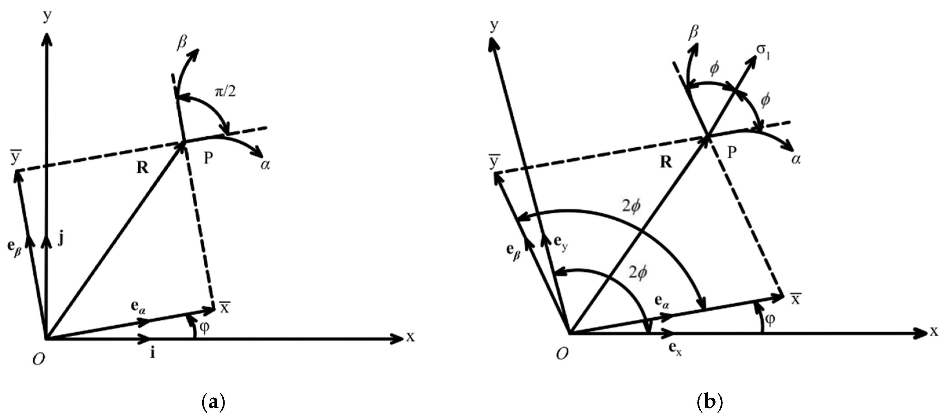
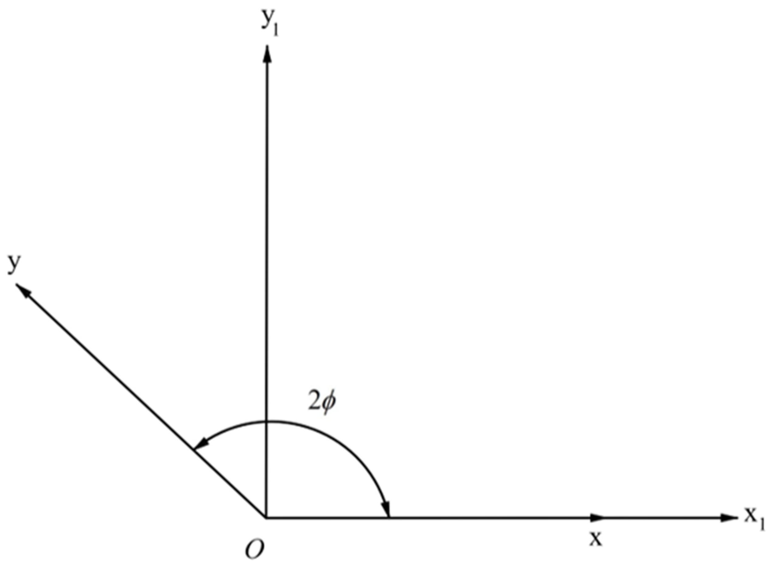
3. Generalized Moving Coordinates

The moving coordinates $\left(\overline{x}, \overline{y}\right)$ are used for solving boundary value problems in pressure-independent plasticity. This method has been described in many monographs, for example, [24]. In short, $\overline{x}$ and $\overline{y}$ are the coordinates of the point C under consideration, referred to axes passing through the origin O and parallel to the characteristic directions at C. The geometric interpretation of the moving coordinates is shown in Figure 1a. In the case of pressure-independent plasticity, the characteristic directions are orthogonal. Therefore, the moving coordinates are orthogonal. It is seen from Equations (6) and (7) that the characteristic directions are not orthogonal if $\lambda \ne 0$.

The geometric interpretation of the generalized moving coordinates, which are also denoted as $\left(\stackrel{-}{x},\stackrel{-}{y}\right),$ is shown in Figure 1b. In this figure, $\left(x, y\right)$ is a skew rectilinear coordinate system with the origin at O. The $x-$axis is tangent to the base $\alpha -$characteristic line passing through O, and the $y-$axis is tangent to the base $\beta -$characteristic line passing through O. Let $e_x$ and $e_y$ be the unit base vectors of the $\left(x, y\right)-$coordinate system. The unit vectors $e_{\mathsf{\alpha }}$ and $e_{\mathsf{\beta }}$ are directed along the $\alpha -$ and $\beta -$characteristic lines at the point C under consideration. Therefore, the angle between the vectors $e_x$ and $e_{\mathsf{\alpha }}$ is $\phi$. Then (Figure 1b):

$$\begin{array}{l}{e}_{\mathsf{\alpha }}\cdot e_x=\cos \phi ,\hspace{1em}{e}_{\mathsf{\alpha }}\cdot e_y=\cos \left(\phi -2\varphi \right),\hspace{1em}{e}_{\mathsf{\beta }}\cdot e_x=\cos \left(\phi +2\varphi \right),\hspace{1em}\\ e_{\mathsf{\beta }}\cdot e_y=\cos \phi ,\hspace{1em}{e}_y\cdot e_x=\cos 2\varphi .\end{array}$$

(14)

The position vector of any point can be represented as

$$R=x{e}_x+y{e}_y=\overline{x}{e}_{\mathsf{\alpha }}+\overline{y}{e}_{\mathsf{\beta }}.$$

(15)

Using Equations (14) and (15), one can find the scalar products, $R\cdot e_x$ and $R\cdot e_y$, as:

$$\begin{array}{l}R\cdot e_x=x+y\cos 2\varphi =\overline{x}\cos \phi +\overline{y}\cos \left(\phi +2\varphi \right),\\ R\cdot e_y=x\cos 2\varphi +y=\overline{x}\cos \left(\phi -2\varphi \right)+\overline{y}\cos \phi .\end{array}$$

(16)

Solving these equations for $\overline{x}$ and $\overline{y}$ yields:

$$\begin{array}{l}\overline{x}=x\frac{\left[\cos \phi -\cos 2\varphi \cos \left(\phi +2\varphi \right)\right]}{{\sin }^{2}2\varphi }+y\frac{\left[\cos \phi \cos 2\varphi -\cos \left(\phi +2\varphi \right)\right]}{{\sin }^{2}2\varphi },\\ \overline{y}=x\frac{\left[\cos \phi \cos 2\varphi -\cos \left(\phi -2\varphi \right)\right]}{{\sin }^{2}2\varphi }+y\frac{\left[\cos \phi -\cos 2\varphi \cos \left(\phi -2\varphi \right)\right]}{{\sin }^{2}2\varphi }.\end{array}$$

(17)

Alternatively, the equations in (16) can be solved for $x$ and $y$. As a result,

$$\begin{array}{l}x=\overline{x}\frac{\left[\cos \phi -\cos 2\varphi \cos \left(\phi -2\varphi \right)\right]}{{\sin }^{2}2\varphi }+\overline{y}\frac{\left[\cos \left(\phi +2\varphi \right)-\cos \phi \cos 2\varphi \right]}{{\sin }^{2}2\varphi },\\ y=\overline{x}\frac{\left[\cos \left(\phi -2\varphi \right)-\cos \phi \cos 2\varphi \right]}{{\sin }^{2}2\varphi }+\overline{y}\frac{\left[\cos \phi -\cos 2\varphi \cos \left(\phi +2\varphi \right)\right]}{{\sin }^{2}2\varphi }.\end{array}$$

(18)

Differentiating the first equation in (17) with respect to $\beta$ and the second with respect to $\alpha$ leads to:

$$\begin{array}{l}{\sin }^{2}2\varphi \frac{\partial \overline{x}}{\partial \beta }=\left[\cos \phi -\cos 2\varphi \cos \left(\phi +2\varphi \right)\right]\frac{\partial x}{\partial \beta }+\left[\cos \phi \cos 2\varphi -\cos \left(\phi +2\varphi \right)\right]\frac{\partial y}{\partial \beta }-\\ \left\{x\left[\sin \phi -\cos 2\varphi \sin \left(\phi +2\varphi \right)\right]+y\left[\sin \phi \cos 2\varphi -\sin \left(\phi +2\varphi \right)\right]\right\}\frac{\partial \phi }{\partial \beta },\\ {\sin }^{2}2\varphi \frac{\partial \overline{y}}{\partial \alpha }=\left[\cos \phi \cos 2\varphi -\cos \left(\phi -2\varphi \right)\right]\frac{\partial x}{\partial \alpha }+\left[\cos \phi -\cos 2\varphi \cos \left(\phi -2\varphi \right)\right]\frac{\partial y}{\partial \alpha }-\\ \left\{x\left[\sin \phi \cos 2\varphi -\sin \left(\phi -2\varphi \right)\right]+y\left[\sin \phi -\cos 2\varphi \sin \left(\phi -2\varphi \right)\right]\right\}\frac{\partial \phi }{\partial \alpha }.\end{array}$$

(19)

It is seen from Equation (13) that $\partial \phi /\partial \alpha =\partial \phi /\partial \beta =\sin 2\varphi$. Therefore, Equation (19) becomes:

$$\begin{array}{l}\frac{\partial \overline{x}}{\partial \beta }=\frac{\left[\cos \phi -\cos 2\varphi \cos \left(\phi +2\varphi \right)\right]}{{\sin }^{2}2\varphi }\frac{\partial x}{\partial \beta }+\frac{\left[\cos \phi \cos 2\varphi -\cos \left(\phi +2\varphi \right)\right]}{{\sin }^{2}2\varphi }\frac{\partial y}{\partial \beta }-\\ \left\{x\left[\sin \phi -\cos 2\varphi \sin \left(\phi +2\varphi \right)\right]+y\left[\sin \phi \cos 2\varphi -\sin \left(\phi +2\varphi \right)\right]\right\}\csc 2\varphi ,\\ \frac{\partial \overline{y}}{\partial \alpha }=\frac{\left[\cos \phi \cos 2\varphi -\cos \left(\phi -2\varphi \right)\right]}{{\sin }^{2}2\varphi }\frac{\partial x}{\partial \alpha }+\frac{\left[\cos \phi -\cos 2\varphi \cos \left(\phi -2\varphi \right)\right]}{{\sin }^{2}2\varphi }\frac{\partial y}{\partial \alpha }-\\ \left\{x\left[\sin \phi \cos 2\varphi -\sin \left(\phi -2\varphi \right)\right]+y\left[\sin \phi -\cos 2\varphi \sin \left(\phi -2\varphi \right)\right]\right\}\csc 2\varphi .\end{array}$$

(20)

Using Equation (18), one can get after some trigonometry:

$$\begin{array}{l}\left\{x\left[\sin \phi -\cos 2\varphi \sin \left(\phi +2\varphi \right)\right]+y\left[\sin \phi \cos 2\varphi -\sin \left(\phi +2\varphi \right)\right]\right\}\csc 2\varphi =-\left(\overline{y}+\overline{x}\cos 2\varphi \right),\\ \left\{x\left[\sin \phi \cos 2\varphi -\sin \left(\phi -2\varphi \right)\right]+y\left[\sin \phi -\cos 2\varphi \sin \left(\phi -2\varphi \right)\right]\right\}\csc 2\varphi =\overline{y}\cos 2\varphi +\overline{x}.\end{array}$$

(21)

Equation (6) can be rewritten using Equation (10) as:

$$\frac{\partial y_1}{\partial \alpha }=\tan \phi \frac{\partial x_1}{\partial \alpha } \mathrm{and} \frac{\partial y_1}{\partial \beta }=\tan \left(\phi +2\varphi \right)\frac{\partial x_1}{\partial \beta }.$$

(22)

One can situate the origin of the $\left(x_1,y_1\right)-$coordinate system at the origin of the $\left(x,y\right)-$coordinate system and direct the $x_1-$axis along the $x-$axis (Figure 2). Then,

$$x=x_1-y_1\cot 2\varphi \mathrm{and} y=\frac{y_1}{\sin 2\varphi }.$$

(23)

Differentiating, one arrives at:

$$\begin{array}{l}\frac{\partial x}{\partial \alpha }=\frac{\partial x_1}{\partial \alpha }+\frac{\partial y_1}{\partial \alpha }\cot 2\varphi ,\hspace{1em}\frac{\partial x}{\partial \beta }=\frac{\partial x_1}{\partial \beta }+\frac{\partial y_1}{\partial \beta }\cot 2\varphi ,\hspace{1em}\\ \frac{\partial y}{\partial \alpha }=\frac{1}{\sin 2\varphi }\frac{\partial y_1}{\partial \alpha }, \hspace{1em}\frac{\partial y}{\partial \beta }=\frac{1}{\sin 2\varphi }\frac{\partial y_1}{\partial \beta }.\end{array}$$

(24)

Consider the terms of the equations in (20) containing the derivatives $\partial x/\partial \alpha$, $\partial y/\partial \alpha$, $\partial x/\partial \beta$, and $\partial y/\partial \beta$. Using Equations (22) and (24), one can represent these terms as:

$$\begin{array}{l}\frac{\left[\cos \phi \cos 2\varphi -\cos \left(\phi -2\varphi \right)\right]}{{\sin }^{2}2\varphi }\frac{\partial x}{\partial \alpha }+\frac{\left[\cos \phi -\cos 2\varphi \cos \left(\phi -2\varphi \right)\right]}{{\sin }^{2}2\varphi }\frac{\partial y}{\partial \alpha }=\\ \left\{\begin{array}{l}\left[\cos \phi \cos 2\varphi -\cos \left(\phi -2\varphi \right)\right]\left(\cot \phi -\cos 2\varphi \right)+\\ \left[\cos \phi -\cos 2\varphi \cos \left(\phi -2\varphi \right)\right]\csc 2\varphi \end{array}\right\}{\csc }^{2}2\varphi \frac{\partial y_1}{\partial \alpha },\\ \frac{\left[\cos \phi -\cos 2\varphi \cos \left(\phi +2\varphi \right)\right]}{{\sin }^{2}2\varphi }\frac{\partial x}{\partial \beta }+\frac{\left[\cos \phi \cos 2\varphi -\cos \left(\phi +2\varphi \right)\right]}{{\sin }^{2}2\varphi }\frac{\partial y}{\partial \beta }=\\ \left\{\begin{array}{l}\left[\cos \phi -\cos 2\varphi \cos \left(\phi +2\varphi \right)\right]\left[\cot \left(\phi +2\varphi \right)-\cot 2\varphi \right]+\\ \left[\cos \phi \cos 2\varphi -\cos \left(\phi +2\varphi \right)\right]\csc 2\varphi \end{array}\right\}{\csc }^{2}2\varphi \frac{\partial y_1}{\partial \alpha }\end{array}$$

(25)

Using trigonometric identities, one can show that the coefficient of $\partial y_1/\partial \alpha$ vanishes in each of these equations. Therefore, Equations (20) and (22) combine to give:

$$\frac{\partial \overline{x}}{\partial \beta }-\left(\overline{y}+\overline{x}\cos 2\varphi \right)=0 \mathrm{and} \frac{\partial \overline{y}}{\partial \alpha }+\overline{y}\cos 2\varphi +\overline{x}=0.$$

(26)

Introduce new variables $\overline{X}$ and $\overline{Y}$ as

$$\overline{x}=\overline{X}\exp \left[\left(\beta -\alpha \right)\cos 2\varphi \right] \mathrm{and} \overline{y}=\overline{Y}\exp \left[\left(\beta -\alpha \right)\cos 2\varphi \right].$$

(27)

Substituting Equation (27) into Equation (26) yields:

$$\frac{\partial \overline{X}}{\partial \beta }-\overline{Y}=0 \mathrm{and} \frac{\partial \overline{Y}}{\partial \alpha }+\overline{X}=0.$$

(28)

It is seen from this equation that the quantities $\overline{X}$ and $\overline{Y}$ separately satisfy the equation of telegraphy. The latter is integrated by the method of Riemann.

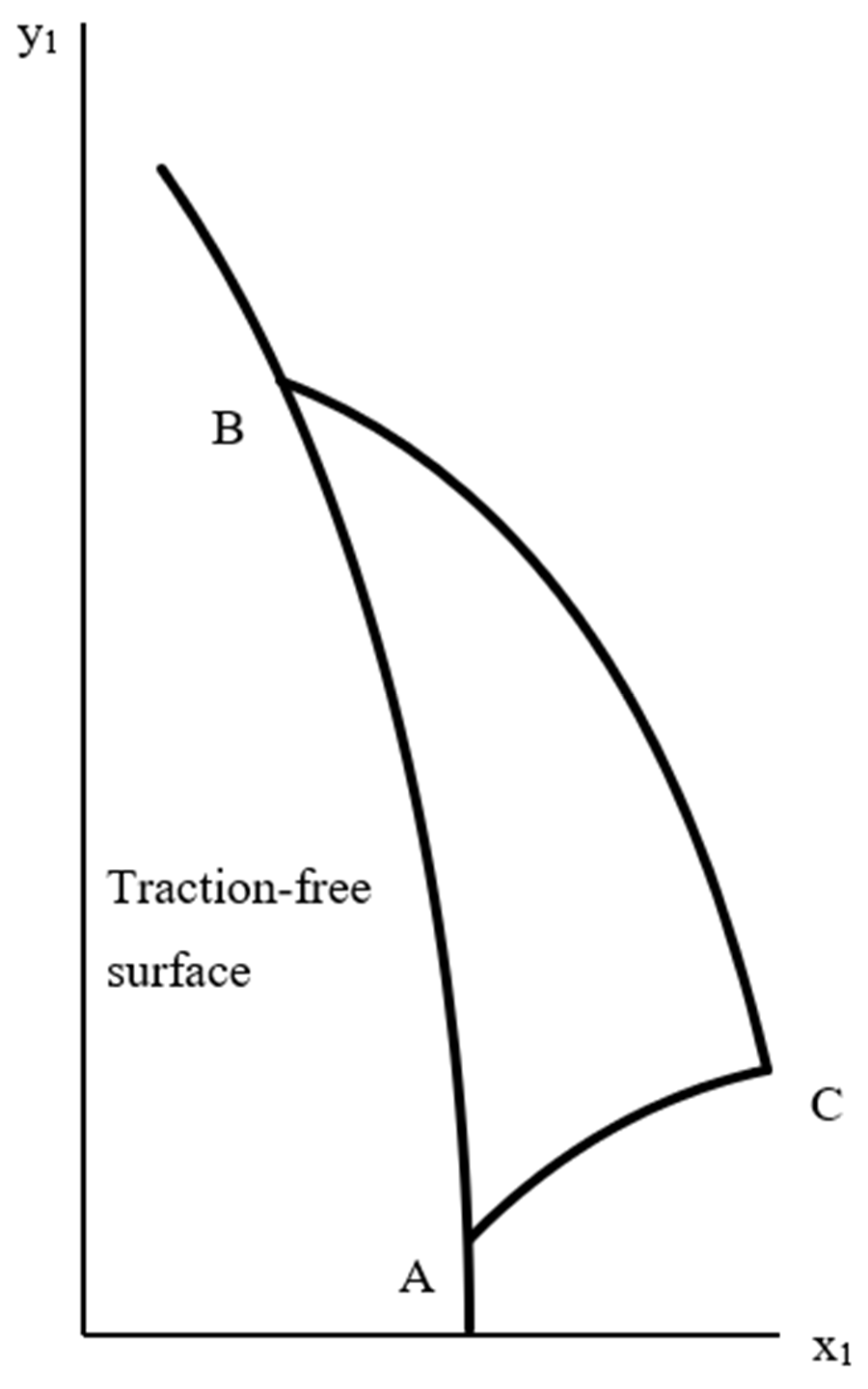
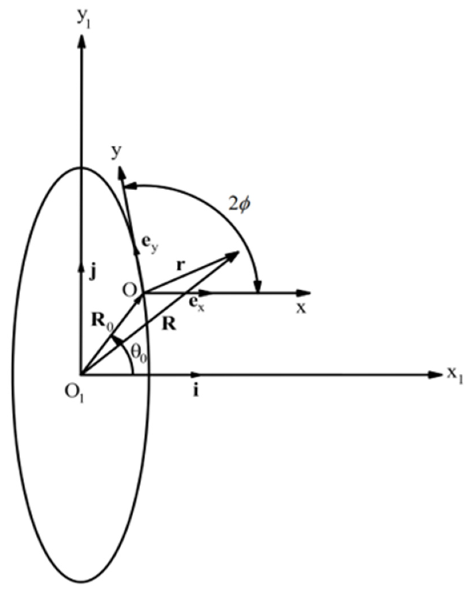
4. Solution near a Traction-Free Surface

One of the principal stresses vanishes on any traction-free surface. The other principal stress and p are determined from Equations (1) and (2). It is necessary to consider two cases. One of these cases demands:

$${\sigma }_1=0, {\sigma }_2=-\frac{2}{1+\lambda }, \mathrm{and} p=\frac{1}{1+\lambda }$$

(29)

on a traction-free surface. The other case demands:

$${\sigma }_2=0, {\sigma }_1=\frac{2}{1-\lambda }, \mathrm{and} p=-\frac{1}{1-\lambda }$$

(30)

on a traction-free surface.

Consider Equation (29). The general structure of the solution is shown in Figure 3. It is required to find $\overline{X}$ and $\overline{Y}$ at a point C. BC is an $\alpha -$characteristic line, and AC is a $\beta -$characteristic line. Riemann’s method for the telegraph equation results in

$${\displaystyle \underset{BCA}{\oint }\left(G\frac{\partial f}{\partial \alpha }-f\frac{\partial G}{\partial \alpha }\right)d\alpha +\left(f\frac{\partial G}{\partial \beta }-G\frac{\partial f}{\partial \beta }\right)d\beta }=0.$$

(31)

Here f is $\overline{X}$ or $\overline{Y}$ and.

$$G\left({\alpha }_C,{\beta }_C,\alpha ,\beta \right)\equiv J_0\left[2\sqrt{\left({\alpha }_C-\alpha \right)\left({\beta }_C-\beta \right)}\right].$$

(32)

Also, $J_0\left(z\right)$ is the Bessel function of the first kind of zero order, ${\alpha }_C$ is the value of $\alpha$ at the point C, and ${\beta }_C$ is the value of $\beta$ at the point C. Note that

$$J_0\left(0\right)=1. \mathrm{and} J_1\left(0\right)=0$$

(33)

where $J_1\left(z\right)=-d{J}_0\left(z\right)/dz$ is the Bessel function of the first kind of first order.

Since $d\beta =0$ on BC and $d\alpha =0$ on AC, Equation (31) can be rewritten as:

$$\begin{array}{l}{\displaystyle \underset{BCA}{\oint }\left(G\frac{\partial f}{\partial \alpha }-f\frac{\partial G}{\partial \alpha }\right)d\alpha +\left(f\frac{\partial G}{\partial \beta }-G\frac{\partial f}{\partial \beta }\right)d\beta }={\displaystyle \underset{{\alpha }_B}{\overset{{\alpha }_C}{\int }}\left(G\frac{\partial f}{\partial \alpha }-f\frac{\partial G}{\partial \alpha }\right)d\alpha }+\\ {\displaystyle \underset{{\beta }_C}{\overset{{\beta }_A}{\int }}\left(f\frac{\partial G}{\partial \beta }-G\frac{\partial f}{\partial \beta }\right)d\beta }+{\displaystyle \underset{AB}{\int }\left(G\frac{\partial f}{\partial \alpha }-f\frac{\partial G}{\partial \alpha }\right)d\alpha +\left(f\frac{\partial G}{\partial \beta }-G\frac{\partial f}{\partial \beta }\right)d\beta }=0.\end{array}$$

(34)

Moreover, $\beta ={\beta }_C$ on BC and $\alpha ={\alpha }_C$ on AC. Therefore, $z=0$ on these lines. Then, it follows from Equations (33) and (34) that:

$$f_C=\frac{f_B+f_A}{2}-\frac{1}{2}{\displaystyle \underset{AB}{\int }\left(G\frac{\partial f}{\partial \alpha }-f\frac{\partial G}{\partial \alpha }\right)d\alpha +\left(f\frac{\partial G}{\partial \beta }-G\frac{\partial f}{\partial \beta }\right)d\beta }.$$

(35)

Here $f_A$, $f_B$, and $f_C$ are the value of f at A, B, and C, respectively.

Put $p_0=1/\left(1+\lambda \right)$ in (12). Then, it follows from Equations (12), (13), and (29) that:

$$P=0, dP=0, d\beta =\frac{d\phi }{2\sin 2\varphi }, \mathrm{and} d\alpha =\frac{d\phi }{2\sin 2\varphi }$$

(36)

on AB.

Using Equation (36), one can rewrite the integral in Equation (35) as

$$\begin{array}{l}{\displaystyle \underset{AB}{\int }\left(G\frac{\partial f}{\partial \alpha }-f\frac{\partial G}{\partial \alpha }\right)d\alpha +\left(f\frac{\partial G}{\partial \beta }-G\frac{\partial f}{\partial \beta }\right)d\beta }=\\ =\frac{1}{2\sin 2\varphi }{\displaystyle \underset{AB}{\int }\left(G\frac{\partial f}{\partial \alpha }-f\frac{\partial G}{\partial \alpha }+f\frac{\partial G}{\partial \beta }-G\frac{\partial f}{\partial \beta }\right)d\phi }.\end{array}$$

(37)

It follows from Equation (13) that:

$$\frac{\partial }{\partial \alpha }=\sin 2\varphi \left(\frac{\partial }{\partial \phi }-\frac{\partial }{\partial P}\right) \mathrm{and} \frac{\partial }{\partial \beta }=\sin 2\varphi \left(\frac{\partial }{\partial \phi }+\frac{\partial }{\partial P}\right).$$

(38)

Equations (37) and (38) combine to give:

$${\displaystyle \underset{AB}{\int }\left(G\frac{\partial f}{\partial \alpha }-f\frac{\partial G}{\partial \alpha }\right)d\alpha +\left(f\frac{\partial G}{\partial \beta }-G\frac{\partial f}{\partial \beta }\right)d\beta }={\displaystyle \underset{AB}{\int }\left(f\frac{\partial G}{\partial P}-G\frac{\partial f}{\partial P}\right)d\phi }.$$

(39)

The derivative $\partial f/\partial P$ can be eliminated using Equation (28). In particular, it follows from Equations (28) and (38) that:

$$\begin{array}{l}\frac{\partial \overline{Y}}{\partial P}=\frac{\partial \overline{Y}}{\partial \phi }-\csc 2\varphi \frac{\partial \overline{Y}}{\partial \alpha }=\frac{\partial \overline{Y}}{\partial \phi }+\overline{X}\csc 2\varphi ,\\ \frac{\partial \overline{X}}{\partial P}=\csc 2\varphi \frac{\partial \overline{X}}{\partial \beta }-\frac{\partial \overline{X}}{\partial \phi }=\overline{Y}\csc 2\varphi -\frac{\partial \overline{X}}{\partial \phi }.\end{array}$$

(40)

Moreover, by replacing $\alpha$ and $\beta$ in Equation (32) with $\phi$ and P using Equation (13), one gets:

$$G\left({\phi }_C,P_C,\phi ,P\right)\equiv J_0\left(Z\right)$$

(41)

where ${\phi }_C$ is the value of $\phi$ at C, $P_C$ is the value of P at C, and

$$Z=\csc 2\varphi \sqrt{{\left(\phi -{\phi }_C\right)}^2-{\left(P-P_C\right)}^2}.$$

(42)

It follows from Equations (41) and (42) that:

$$\frac{\partial G}{\partial P}=\frac{J_1\left(Z\right)\left(P-P_C\right)}{Z{\sin }^{2}2\varphi } \mathrm{and} \frac{\partial G}{\partial \phi }=-\frac{J_1\left(Z\right)\left(\phi -{\phi }_C\right)}{Z{\sin }^{2}2\varphi }.$$

(43)

Substituting Equation (40) into Equation (39) and integrating by parts, one arrives at:

$$\begin{array}{l}{\displaystyle \underset{AB}{\int }\left(\overline{X}\frac{\partial G}{\partial P}-G\frac{\partial \overline{X}}{\partial P}\right)d\phi }={\displaystyle \underset{AB}{\int }\left[\overline{X}\left(\frac{\partial G}{\partial P}-\frac{\partial G}{\partial \phi }\right)-G\overline{Y}\csc 2\varphi \right]d\phi }+{\overline{X}}_B-{\overline{X}}_A,\\ {\displaystyle \underset{AB}{\int }\left(\overline{Y}\frac{\partial G}{\partial P}-G\frac{\partial \overline{Y}}{\partial P}\right)d\phi }={\displaystyle \underset{AB}{\int }\left[\overline{Y}\left(\frac{\partial G}{\partial P}+\frac{\partial G}{\partial \phi }\right)-G\overline{X}\csc 2\varphi \right]d\phi }-{\overline{Y}}_B+{\overline{Y}}_A.\end{array}$$

(44)

Eliminating here the derivatives $\partial G/\partial P$ and $\partial G/\partial \phi$ using Equation (43) yields:

$$\begin{array}{l}{\displaystyle \underset{AB}{\int }\left(\overline{X}\frac{\partial G}{\partial P}-G\frac{\partial \overline{X}}{\partial P}\right)d\phi }=\csc 2\varphi {\displaystyle \underset{AB}{\int }\left[\overline{X}\frac{J_1\left(Z\right)\left(\phi -{\phi }_C-P_C\right)}{Z\sin 2\varphi }-J_0\left(Z\right)\overline{Y}\right]d\phi }+{\overline{X}}_B-{\overline{X}}_A,\\ {\displaystyle \underset{AB}{\int }\left(\overline{Y}\frac{\partial G}{\partial P}-G\frac{\partial \overline{Y}}{\partial P}\right)d\phi }=-\csc 2\varphi {\displaystyle \underset{AB}{\int }\left[\overline{Y}\frac{J_1\left(Z\right)\left(\phi -{\phi }_C+P_C\right)}{Z\sin 2\varphi }+J_0\left(Z\right)\overline{X}\right]d\phi }-{\overline{Y}}_B+{\overline{Y}}_A.\end{array}$$

(45)

Substituting Equation (45) into Equation (35) leads to:

$$\begin{array}{l}{\overline{X}}_C={\overline{X}}_A-\frac{\csc 2\varphi }{2}{\displaystyle \underset{{\phi }_A}{\overset{{\phi }_B}{\int }}\left[\overline{X}\frac{J_1\left(Z\right)\left(\phi -{\phi }_C-P_C\right)}{Z\sin 2\varphi }-J_0\left(Z\right)\overline{Y}\right]}d\phi ,\\ {\overline{Y}}_C={\overline{Y}}_B+\frac{\csc 2\varphi }{2}{\displaystyle \underset{{\phi }_A}{\overset{{\phi }_B}{\int }}\left[\overline{Y}\frac{J_1\left(Z\right)\left(\phi -{\phi }_C+P_C\right)}{Z\sin 2\varphi }+J_0\left(Z\right)\overline{X}\right]d\phi }.\end{array}$$

(46)

The coefficients of $\overline{X}$ and $\overline{Y}$ in the integrands are known functions of $\phi$ due to Equations (36) and (42).

Consider Equation (30). In this case, AC is an $\alpha -$characteristic line, and BC is a $\beta -$characteristic line (Figure 3). Putting $p_0=-1/\left(1+\lambda \right)$ in Equation (12) and repeating the line of reasoning that has led to Equation (46) in the previous case, one gets:

$$\begin{array}{l}{\overline{X}}_C={\overline{X}}_B+\frac{\csc 2\varphi }{2}{\displaystyle \underset{{\phi }_A}{\overset{{\phi }_B}{\int }}\left[\overline{X}\frac{J_1\left(Z\right)\left(\phi -{\phi }_C-P_C\right)}{Z\sin 2\varphi }-J_0\left(Z\right)\overline{Y}\right]}d\phi ,\\ {\overline{Y}}_C={\overline{Y}}_A-\frac{\csc 2\varphi }{2}{\displaystyle \underset{{\phi }_A}{\overset{{\phi }_B}{\int }}\left[\overline{Y}\frac{J_1\left(Z\right)\left(\phi -{\phi }_C+P_C\right)}{Z\sin 2\varphi }+J_0\left(Z\right)\overline{X}\right]d\phi }.\end{array}$$

(47)

It follows from Equation (11) that:

$$P_C=\frac{{\phi }_A-{\phi }_B}{2} \mathrm{and} {\phi }_C=\frac{{\phi }_B+{\phi }_A}{2}$$

(48)

if Equation (29) is valid and

$$P_C=\frac{{\phi }_B-{\phi }_A}{2} \mathrm{and} {\phi }_C=\frac{{\phi }_B+{\phi }_A}{2}$$

(49)

Equation (30) is valid. Using Equations (48) and (49), one can eliminate ${\phi }_C$ and $P_C$ in Equations (46) and (47).

The free surface geometry determines the quantities $\overline{X}$ and $\overline{Y}$ involved in Equations (46) and (47). Since $P=0$ on the free surface, it is seen from Equations (13) and (27) that:

$$\overline{X}=\overline{x} \mathrm{and} \overline{Y}=\overline{y}$$

(50)

on AB. One of the principal stress directions is orthogonal to the free surface. Therefore, replacing $\phi$ with $\psi$ in Equations (46) and (47) is convenient. It is seen from Equation (10) that $d\psi =d\phi$. Then, using Equations (48)–(50), one rewrites Equations (46) and (47) as:

$$\begin{array}{l}{\overline{X}}_C={\overline{x}}_A-\frac{\csc 2\varphi }{2}{\displaystyle \underset{{\psi }_A}{\overset{{\psi }_B}{\int }}\left[\overline{x}\frac{J_1\left(Z\right)\left(\psi -{\psi }_B\right)}{Z\sin 2\varphi }-J_0\left(Z\right)\overline{y}\right]}d\psi ,\\ {\overline{Y}}_C={\overline{y}}_B+\frac{\csc 2\varphi }{2}{\displaystyle \underset{{\psi }_A}{\overset{{\psi }_B}{\int }}\left[\overline{y}\frac{J_1\left(Z\right)\left(\psi -{\psi }_A\right)}{Z\sin 2\varphi }+J_0\left(Z\right)\overline{x}\right]d\psi },\end{array}$$

(51)

and

$$\begin{array}{l}{\overline{X}}_C={\overline{x}}_B+\frac{\csc 2\varphi }{2}{\displaystyle \underset{{\psi }_A}{\overset{{\psi }_B}{\int }}\left[\overline{x}\frac{J_1\left(Z\right)\left(\psi -{\psi }_B\right)}{Z\sin 2\varphi }-J_0\left(Z\right)\overline{y}\right]}d\psi ,\\ {\overline{Y}}_C={\overline{y}}_A-\frac{\csc 2\varphi }{2}{\displaystyle \underset{{\psi }_A}{\overset{{\psi }_B}{\int }}\left[\overline{y}\frac{J_1\left(Z\right)\left(\psi -{\psi }_A\right)}{Z\sin 2\varphi }+J_0\left(Z\right)\overline{x}\right]d\psi },\end{array}$$

(52)

respectively.

Equations (51) and (52) coincide with the solution [5] for pressure-independent material (i.e., $\varphi =\pi /4$).

5. Numerical Example

The distributions of $\overline{x}$ and $\overline{y}$ along AB are required to evaluate the integrals in Equations (51) and (52). The free surface shape determines these distributions. The numerical solution below is for an elliptic hole. Its equation can be written as:

$$y_1^2+\frac{x_1^2}{a^2}=1 \mathrm{or} \left({\sin }^2\theta +\frac{{\cos }^2\theta }{a^2}\right){\rho }^2=1$$

(53)

where $x_1=\rho \cos \theta$ and $y_1=\rho \sin \theta$. Equations (17) and (18) have been derived upon the assumption that the $x-$axis coincides with the $x_1-$axis. Therefore, the origin of the $\left(x,y\right)-$coordinate system should be situated at a point of the ellipse where the tangent to the $\alpha -$is parallel to the $x_1-$axis. This condition is equivalent to:

$$\psi =\varphi$$

(54)

at the origin of the $\left(x,y\right)-$coordinate system. Let ${\theta }_0$ be the value of $\theta$ at which this condition is satisfied. The components of the unit vector orthogonal to the ellipse are readily determined from Equation (53). As a result,

$$a^2\tan \theta =\tan \psi .$$

(55)

Then, the condition Equation (54) yields:

$$a^2\tan {\theta }_0=\tan \varphi .$$

(56)

The ellipse, $\left(x, y\right)-$coordinate system, and $\left(x_1, y_1\right)-$coordinate system are shown in Figure 4. The unit base vectors of the $\left(x, y\right)-$coordinate system are denoted as $e_x$ and $e_y$, and the unit base vectors of the $\left(x_1, y_1\right)-$coordinate system as i and j. The position vector of a generic point is:

$$R=R_0+r.$$

(57)

Using Equation (56), one can represent the vector $R_0$ as:

$$\begin{array}{l}{R}_0=x_{0}i+y_{0}j,\\ x_0=\frac{a^2\cos \varphi }{\sqrt{1-\left(1-a^2\right){\cos }^2\varphi }},\hspace{1em}{y}_0=\frac{\sin \varphi }{\sqrt{1-\left(1-a^2\right){\cos }^2\varphi }}.\end{array}$$

(58)

It follows from the geometry of Figure 4 that:

$$e_x\cdot i=1,\hspace{1em}{e}_x\cdot j=0,\hspace{1em}{e}_y\cdot i=\cos 2\varphi ,\hspace{1em}{e}_y\cdot j=\sin 2\varphi .$$

(59)

Using Equations (58) and (59), one can find the scalar products $R\cdot i$ and $R\cdot j$ from Equation (57) as:

$$x_1=x_0+x+y\cos 2\varphi \mathrm{and} y_1=y_0+y\sin 2\varphi .$$

(60)

Solving these equations for x and y yields:

$$x=x_1-y_1\cot 2\varphi -x_0+y_0\cot 2\varphi \mathrm{and} y=\frac{y_1-y_0}{\sin 2\varphi }.$$

(61)

It is convenient to rewrite these equations in terms of $\rho$ and $\theta$ as

$$x=\rho \left(\cos \theta -\sin \theta \cot 2\varphi \right)-x_0+y_0\cot 2\varphi \mathrm{and} y=\frac{\rho \sin \theta -y_0}{\sin 2\varphi }.$$

(62)

One can eliminate r in these equations using Equation (54). As a result,

$$\begin{array}{l}x=\frac{a\left(\cos \theta -\sin \theta \cot 2\varphi \right)}{\sqrt{a^2{\sin }^2\theta +{\cos }^2\theta }}-x_0+y_0\cot 2\varphi ,\\ y=\frac{a\sin \theta }{\sin 2\varphi \sqrt{a^2{\sin }^2\theta +{\cos }^2\theta }}-\frac{y_0}{\sin 2\varphi }.\end{array}$$

(63)

Equation (55) allows for x and y to be calculated from Equation (63) as functions of $\psi$. Then, Equations (10) and (17) supply $\overline{x}$ and $\overline{y}$ as functions of $\psi$. These functions have been used in Equation (51) to calculate ${\overline{X}}_C$ and ${\overline{Y}}_C.$ Having ${\overline{X}}_C$ and ${\overline{Y}}_C$, one can calculate the $x_1-$ and $y_1-$coordinates of point C using Equations (18), (27), and (60). The principal stresses at this point are found from Equations (1), (2), (12), and (48) (or (49)). The numerical results below are for Equation (29). Figure 5 depicts the variation of the stress ${\sigma }_1$ along the $x_1-$axis for several values of $\lambda$ and a. Figure 6 shows the variation of the stress ${\sigma }_2$. In these figures, s is the distance from the hole surface, $s=x_1-a$. Figure 5 and Figure 6 reveal a significant effect of $\lambda$ on the stresses. In particular, the effect of a is invisible in these figures. However, the hole shape does affect the stresses near the surface. Figure 7 depicts the variation of the principal stresses for several a-values at $\lambda =-1/4$. It is seen from this figure that the value of $\left|{\sigma }_1\right|$ near a circular hole ($a=1$) is larger than its value near an elliptic hole. However, elliptical holes produce higher values of $\left|{\sigma }_1\right|$ than the corresponding circular hole at some distance from the hole’s surface. The same tendency occurs with the stress $\left|{\sigma }_2\right|$.

6. Conclusions

From this work, the following conclusions can be drawn:

(1)

The generalized method of moving coordinates is efficient for determining stress fields near traction-free surfaces. In particular, determining the stress components at any point of the plastic region requires evaluating one ordinary integral in Equations (51) or (52).

(2)

The solutions in Equations (51) and (52) are independent of other boundary conditions, though the shape of the plastic region is.

(3)

The solution found is identical to the solution in [5] if λ = 0 in Equation (1).

(4)

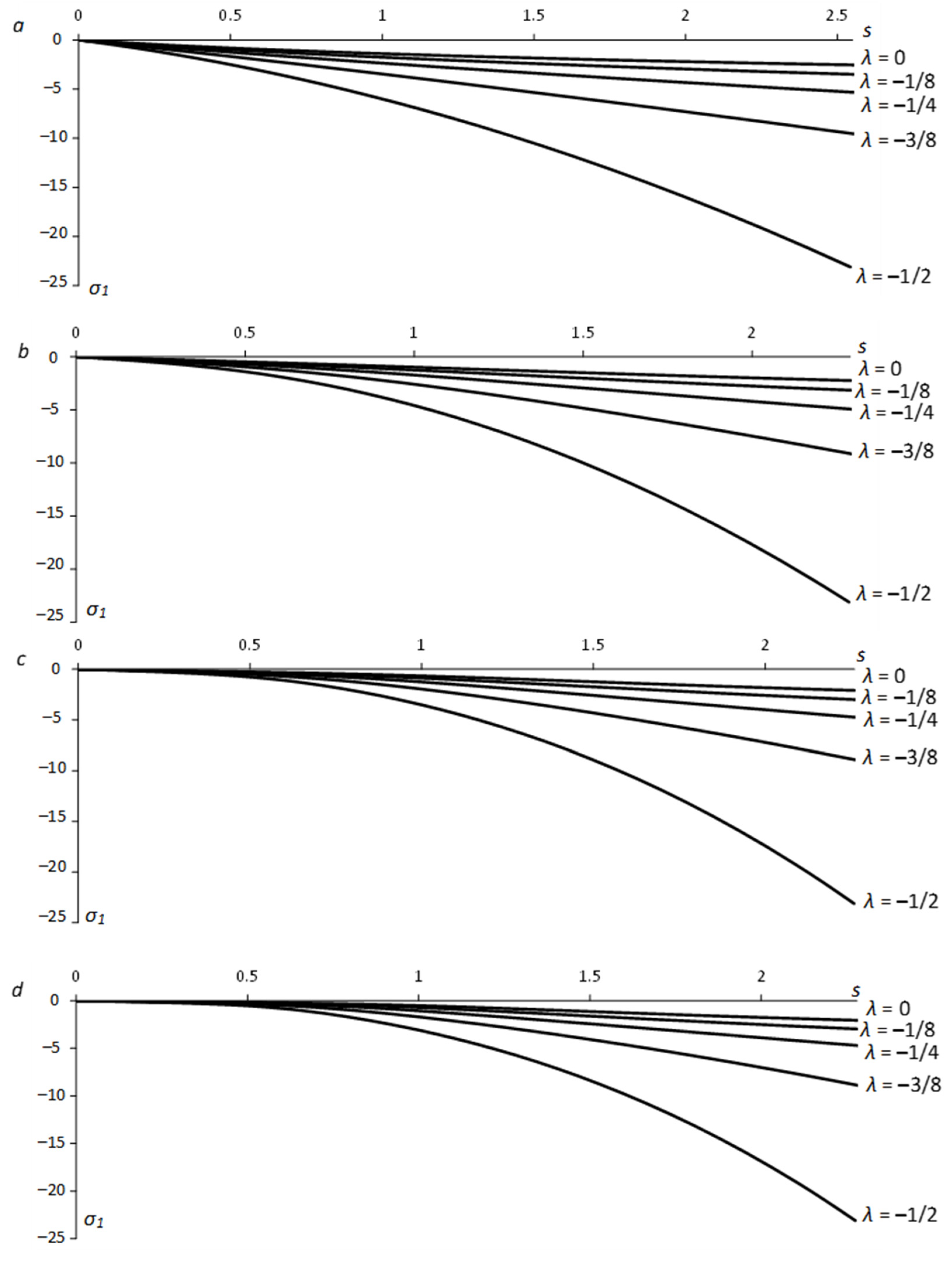
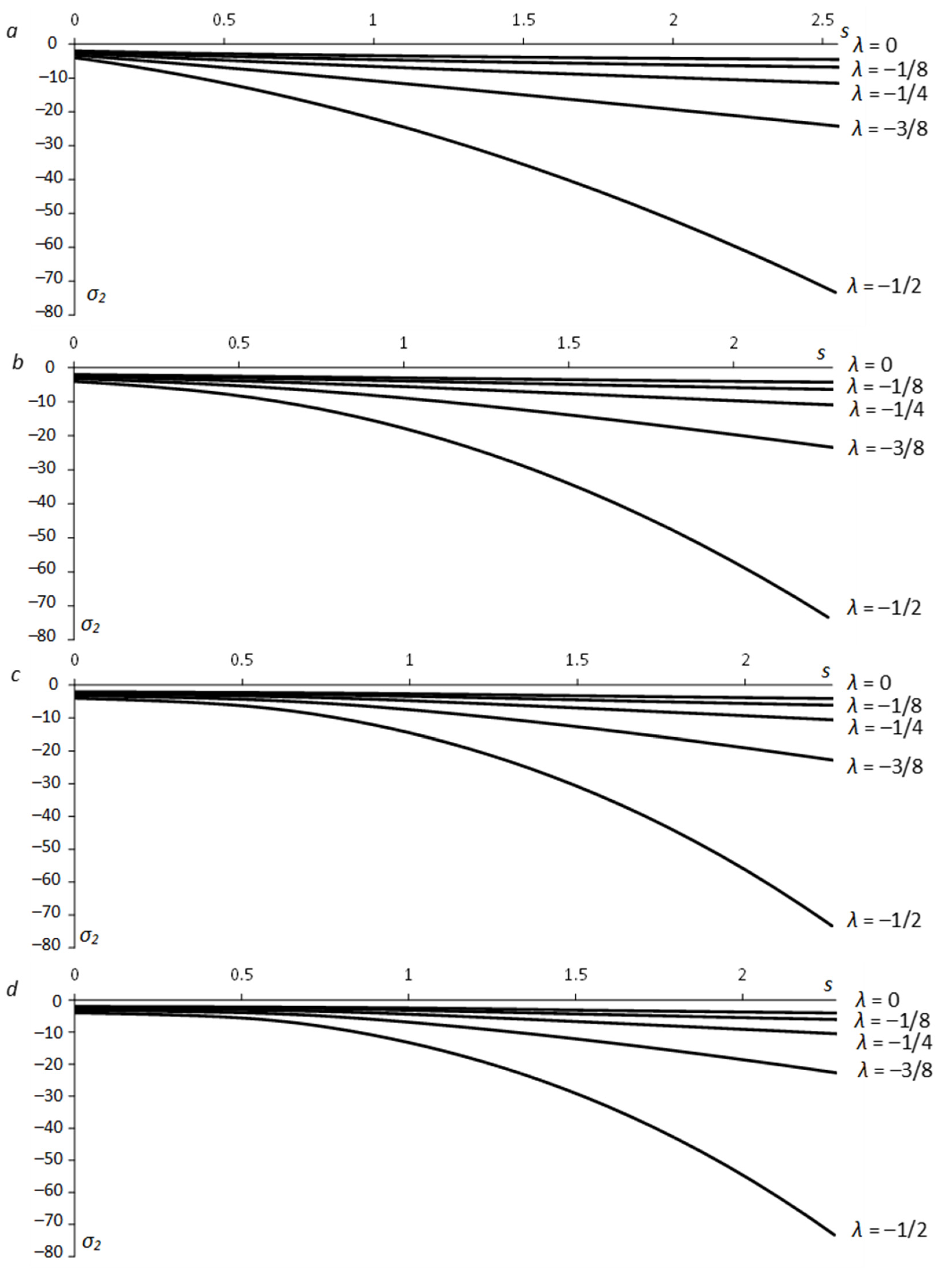
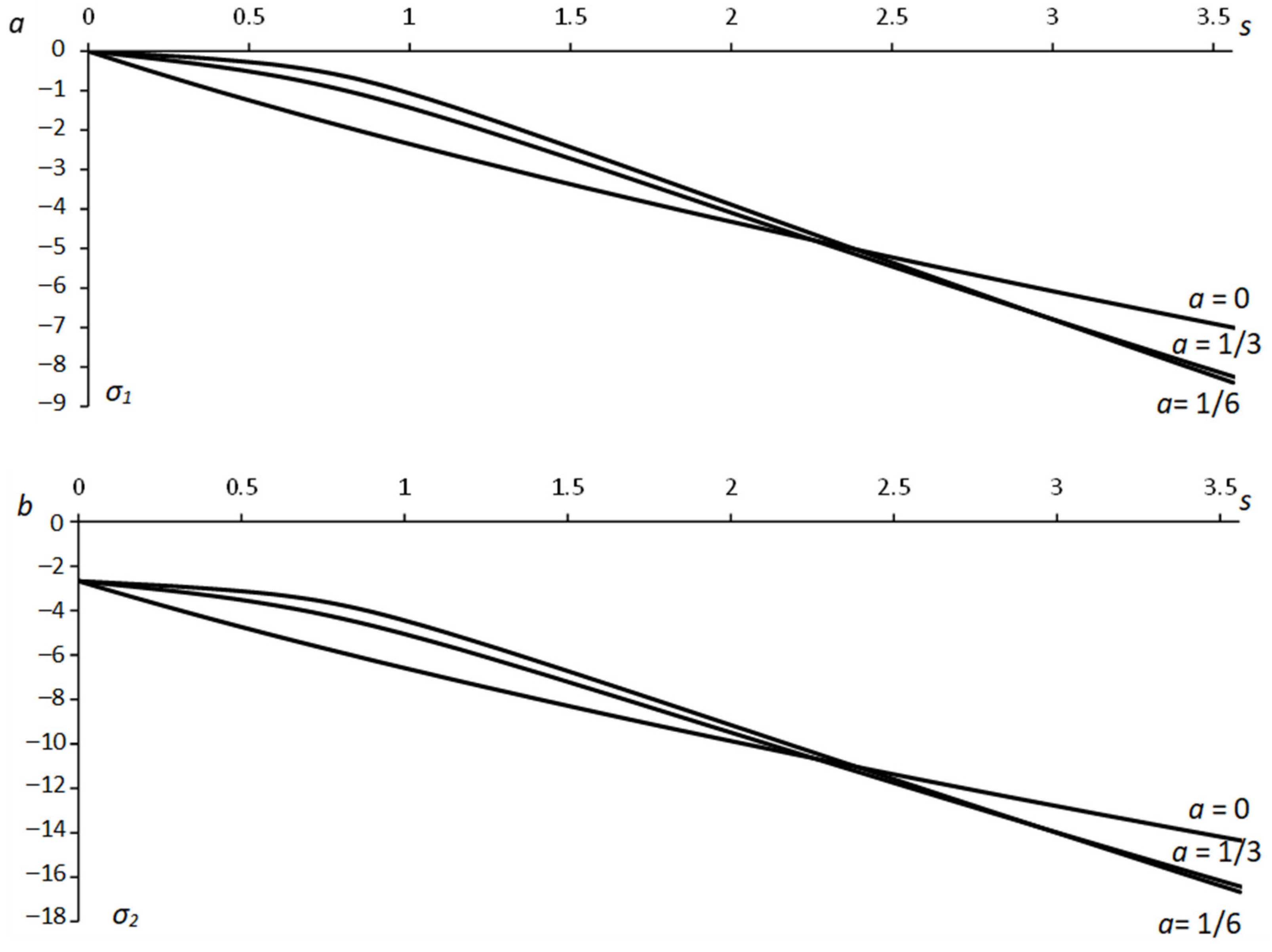
The parameter λ involved in Equation (1) has a much greater effect on the stress field than the aspect ratio (Figure 5 and Figure 6). However, it is a consequence of the yield criterion. For a given material, the aspect ratio affects the stress distribution in a small region near the hole (Figure 7).

(5)

The solution found is for perfectly plastic material. However, slip-line solutions for the class of problems considered agree well with experimental results for strain-hardening materials [25].

References

1. Williams, M.L. On the stress distribution at the base of a stationary crack. J. Appl. Mech. 1956, 24, 109–114. [Google Scholar] [CrossRef]
2. Rice, J.R. A path independent integral and the approximate analysis of strain concentration by notches and cracks. J. Appl. Mech. 1968, 35, 379–386. [Google Scholar] [CrossRef]
3. Li, J.; Hancock, J.W. Mode I and mixed mode fields with incomplete crack tip plasticity. Int. J. Solids Struct. 1999, 36, 711–725. [Google Scholar] [CrossRef]
4. Papanastasiou, P.; Durban, D. Singular plastic fields in non-associative pressure sensitive solids. Int. J. Solids Struct. 2001, 38, 1539–1550. [Google Scholar] [CrossRef]
5. Thomason, P.F. Riemann-Integral solutions for the plastic slip-line fields around elliptical holes. J. Appl. Mech. 1978, 45, 678–679. [Google Scholar] [CrossRef]
6. Thomason, P.F. Ductile fracture and the stability of incompressible plasticity in the presence of microvoids. Acta Metall. 1981, 29, 763–777. [Google Scholar] [CrossRef]
7. Zhang, A.B.; Wang, B.L. Explicit solutions of an elliptic hole or a crack problem in thermoelectric materials. Eng. Fract. Mech. 2016, 151, 11–21. [Google Scholar] [CrossRef]
8. Zhang, A.B.; Wang, B.L.; Wang, J.; Du, J.K. Two-dimensional problem of thermoelectric materials with an elliptic hole or a rigid inclusion. Int. J. Therm. Sci. 2017, 117, 184–195. [Google Scholar] [CrossRef]
9. Tuna, M.; Trovalusci, P. Stress distribution around an elliptic hole in a plate with ‘implicit’ and ‘explicit’ non-local models. Compos. Struct. 2021, 256, 113003. [Google Scholar] [CrossRef]
10. Ostsemin, A.A.; Utkin, P.B. Stress-strain state and stress intensity factors of an inclined elliptic defect in a plate under biaxial loading. Mech. Solids 2010, 45, 214–225. [Google Scholar] [CrossRef]
11. Wang, W.; Yuan, H.; Li, X.; Shi, P. Stress concentration and damage factor due to central elliptical hole in functionally graded panels subjected to uniform tensile traction. Materials 2019, 12, 422. [Google Scholar] [CrossRef]
12. Willis, J.R. The stress field around an elliptical crack in an anisotropic elastic medium. Int. J. Eng. Sci. 1968, 6, 253–263. [Google Scholar] [CrossRef]
13. Huang, Y.-H.; Yang, S.-Q.; Tian, W.-L. Cracking process of a granite specimen that contains multiple pre-existing holes under uniaxial compression. Fatigue Fract. Eng. Mater. Struct. 2019, 42, 1341–1356. [Google Scholar] [CrossRef]
14. Murru, P.T.; Rajagopal, K.R. Stress concentration due to the presence of a hole within the context of elastic bodies. Mat. Des. Process. Commun. 2021, 3, e219. [Google Scholar] [CrossRef]
15. Murru, P.T.; Rajagopal, K.R. Stress concentration due to the bi-axial deformation of a plate of a porous elastic body with a hole. Z. Angew. Math. Mech. 2021, 101, e202100103. [Google Scholar] [CrossRef]
16. Meyer, M.; Sayir, M.B. The elasto-plastic plate with a hole: Analytical solutions derived by singular perturbations. Z. Angew. Math. Phys. 1995, 46, 427–445. [Google Scholar]
17. Yaocai Ma, Y.; Lu, A.; Cai, H. Analytical method for determining the elastoplastic interface of a circular hole subjected to biaxial tension-compression loads. Mech. Based Des. Struct. Mach. 2022, 50, 3206–3223. [Google Scholar] [CrossRef]
18. Li, Z.; Mantell, S.C.; Davidson, J.H. Mechanical analysis of streamlined tubes with non-uniform wall thickness for heat exchangers. J. Strain Anal. Eng. Des. 2005, 40, 275–285. [Google Scholar] [CrossRef]
19. Jafari Fesharaki, J.; Roghani, M. Mechanical behavior and optimization of functionally graded hollow cylinder with an elliptic hole. Mech. Adv. Compos. Struct. 2020, 7, 189–201. [Google Scholar] [CrossRef]
20. Druyanov, B. Technological Mechanics of Porous Bodies; Clarendon Press: New York, NY, USA, 1993. [Google Scholar]
21. Cox, G.M.; Thamwattana, N.; McCue, S.W.; Hill, J.M. Coulomb–Mohr Granular Materials: Quasi-static flows and the highly frictional limit. ASME. Appl. Mech. Rev. 2008, 61, 060802. [Google Scholar] [CrossRef]
22. Burenin, A.A.; Tkacheva, A.V. Piecewise linear plastic potentials as a tool for calculating plane transient temperature stresses. Mech. Solids 2020, 55, 791–799. [Google Scholar] [CrossRef]
23. Spencer, A.J.M. A theory of the kinematics of ideal soils under plane strain conditions. J. Mech. Phys. Solids 1964, 12, 337–351. [Google Scholar] [CrossRef]
24. Hill, R. The Mathematical Theory of Plasticity; Clarendon Press: Oxford, UK, 1950. [Google Scholar]
25. Bastawros, A.; Kyung-Suk, K. Experimental analysis of near-crack-tip plastic flow and deformation characteristics (I): Polycrystalline aluminum. J. Mech. Phys. Solids 2000, 48, 67–98. [Google Scholar] [CrossRef]
Figure 1. Moving coordinates: (a) pressure-independent yield criterion, (b) pressure-dependent yield criterion.
Materials 15 06266 g001
Figure 2. ( x 1 ,   y 1 ) coordinate system chosen for deriving Equation (28).
Materials 15 06266 g002
Figure 3. Illustration of the general boundary value problem.
Materials 15 06266 g003
Figure 4. Illustration of the boundary value problem for an elliptic hole.
Materials 15 06266 g004
Figure 5. Dependence of the principal stress σ1 on the distance from the free surface along the x1-axis for several λ-values: (a) a = 1 (circular hole), (b) a = 1/2, (c) a = 1/4, (d) a = 1/6.
Materials 15 06266 g005
Figure 6. Dependence of the principal stress σ2 on the distance from the free surface along the x1-axis for several λ-values: (a) a = 1 (circular hole), (b) a = 1/2, (c) a = 1/4, (d) a = 1/6.
Materials 15 06266 g006
Figure 7. Dependence of the principal stress on the distance from the free surface along the x1-axis for several a-values at λ = −1/4: (a) σ1-stress, (b) σ2-stress.
Materials 15 06266 g007
Publisher’s Note: MDPI stays neutral with regard to jurisdictional claims in published maps and institutional affiliations.