

Stress Concentration Factors of Concrete-Filled T-Joints under In-Plane Bending: Experiments, FE Analysis and Formulae

Abstract
:1. Introduction
2. Experimental Program
2.1. Specimens and Material Properties
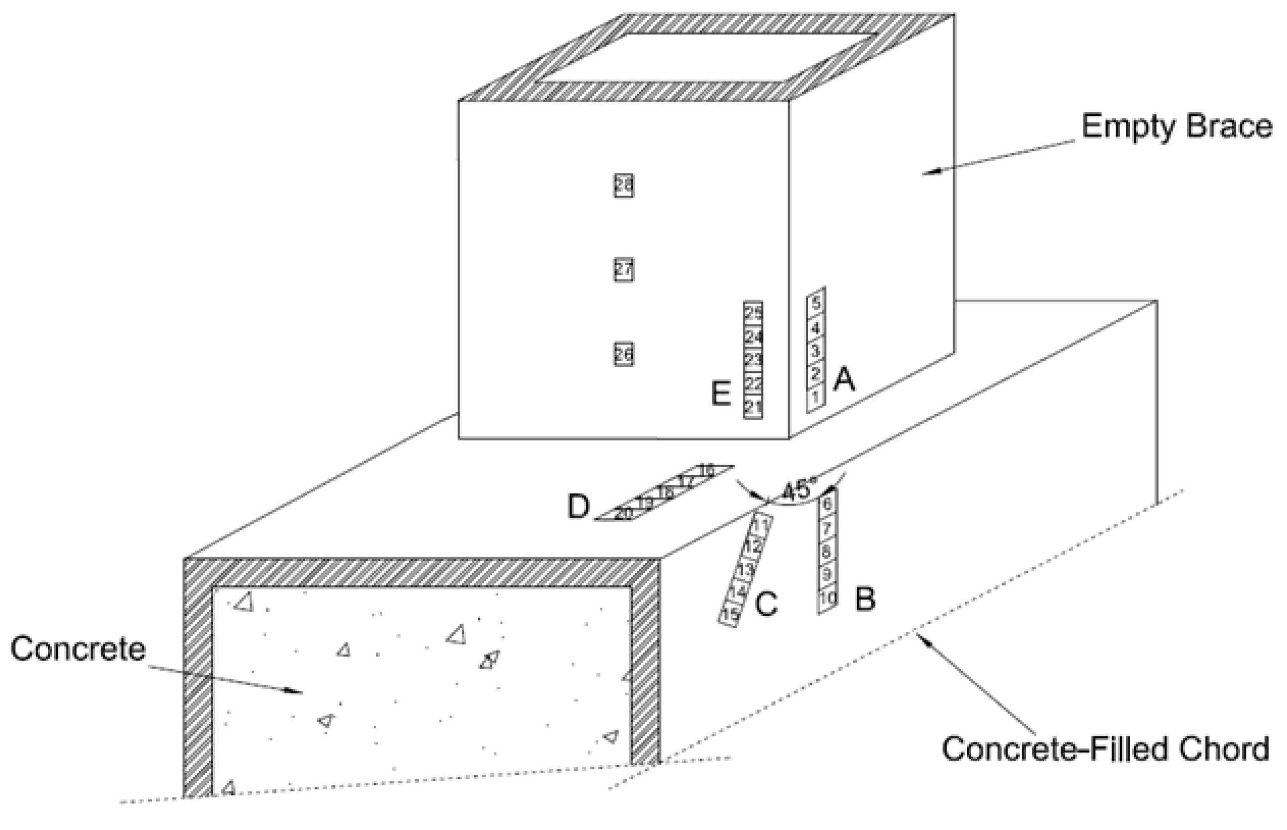
2.2. Instrumentation, Test Setup, and Loading
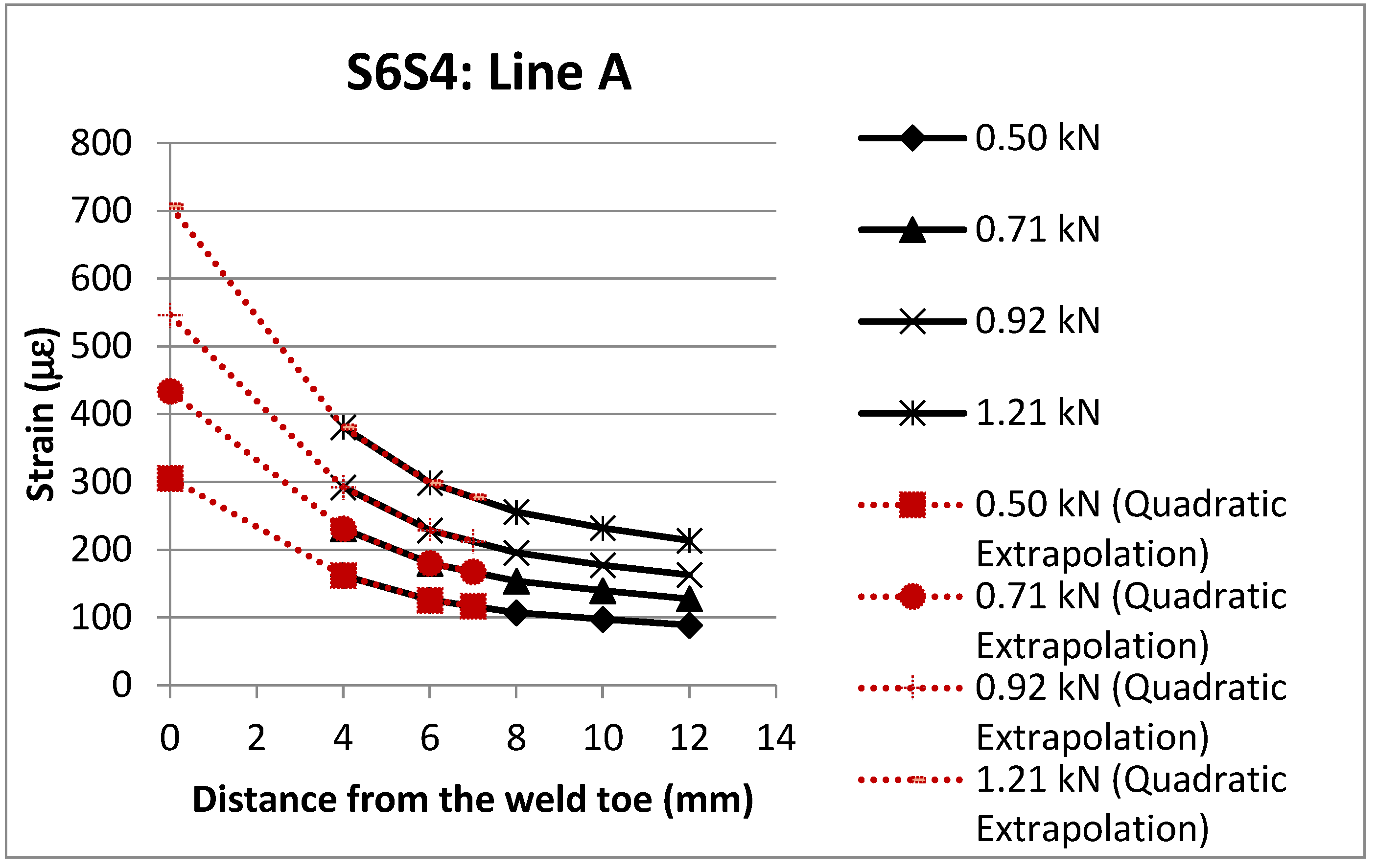
2.3. Experimental SCF
3. Finite Element Analysis (FEA)
3.1. General
3.2. Material Properties, Interaction, and Loading
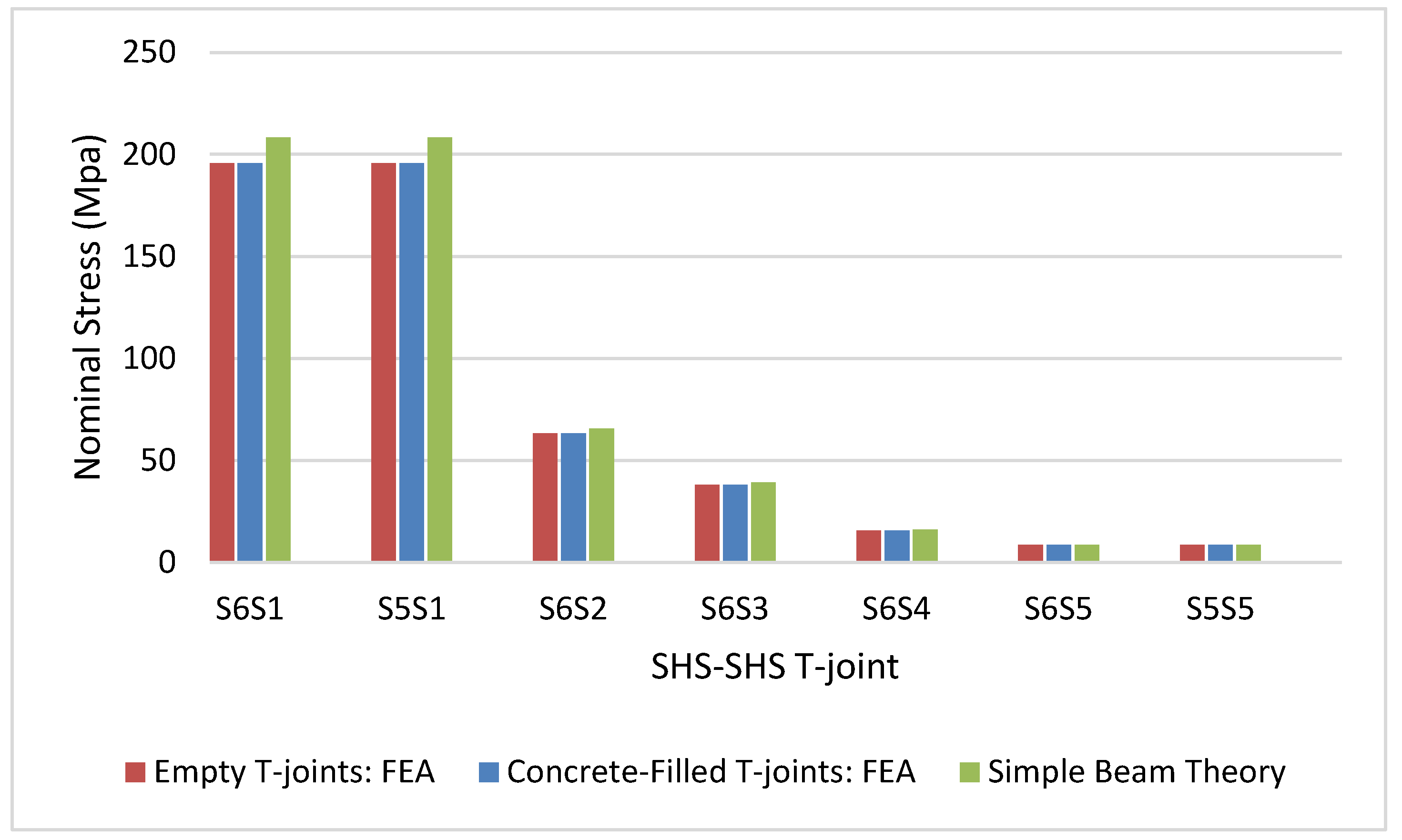
3.3. Numerical SCF
4. Results
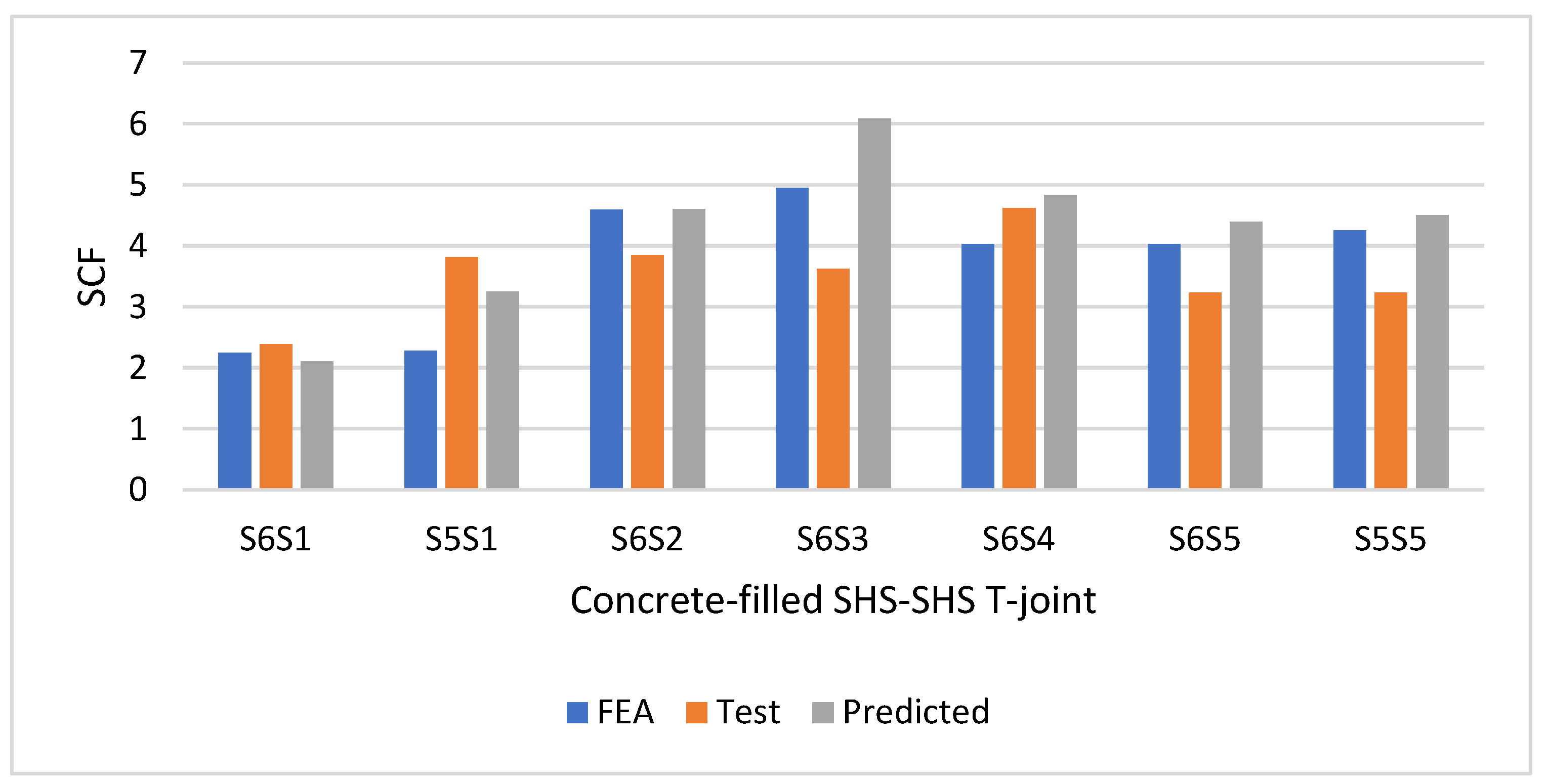
4.1. SCFs
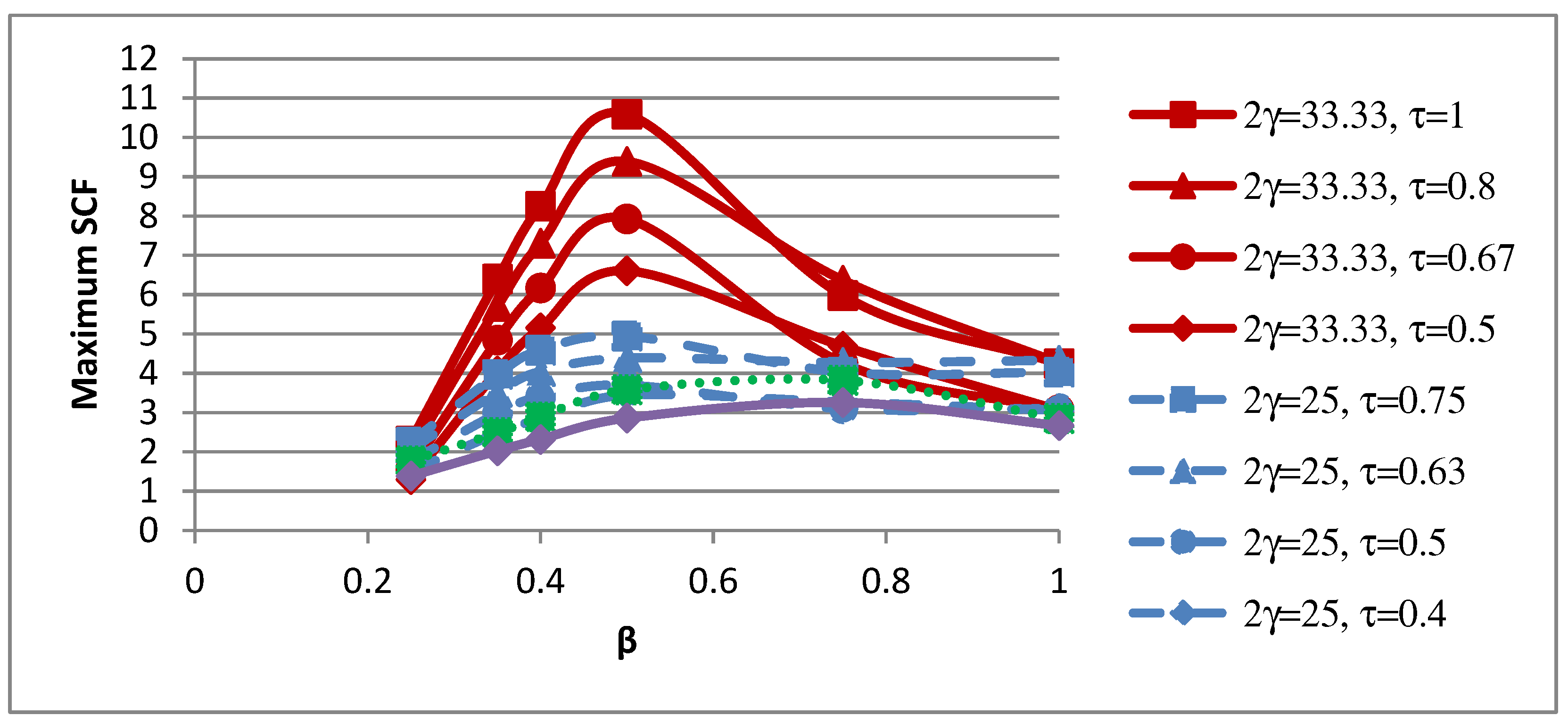
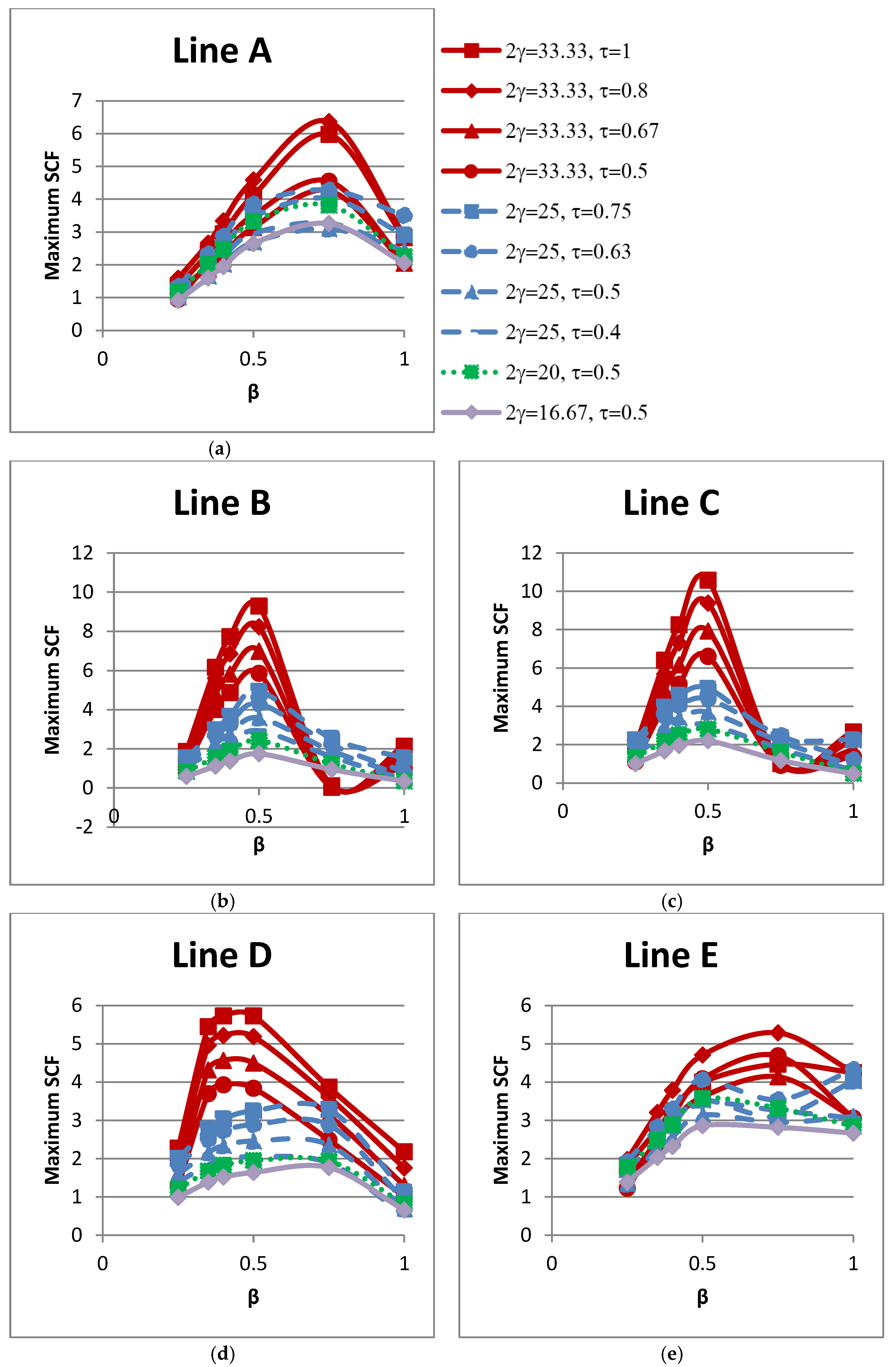
4.2. Influence of β on SCFs
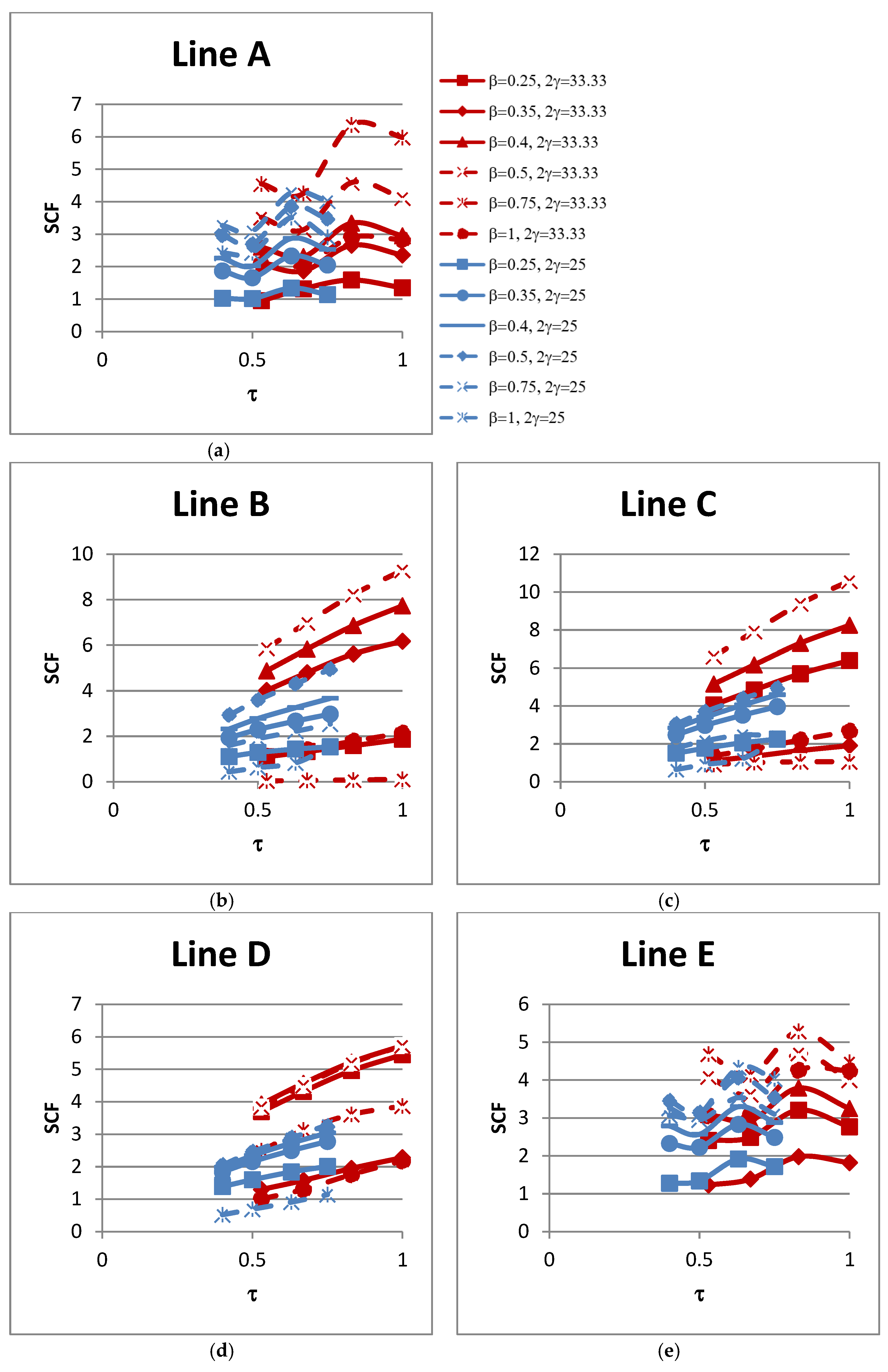
4.3. Influence of τ on SCFs
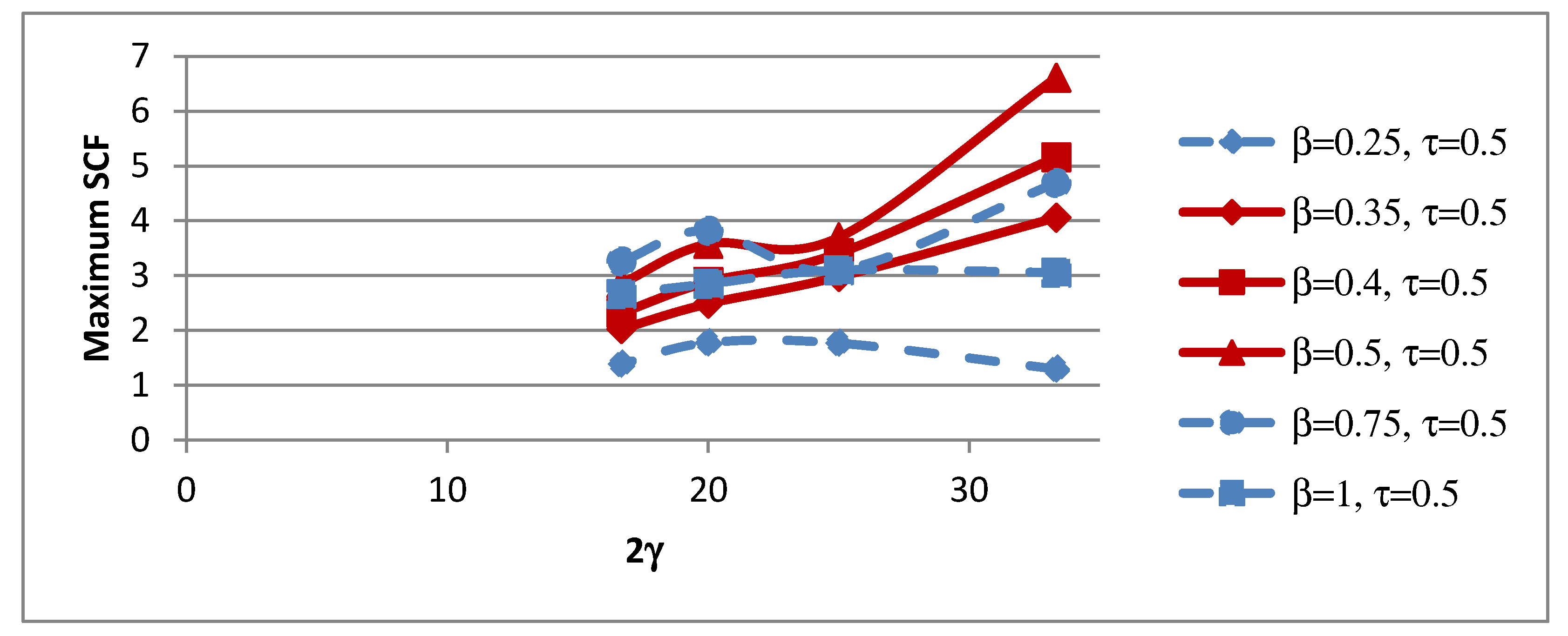
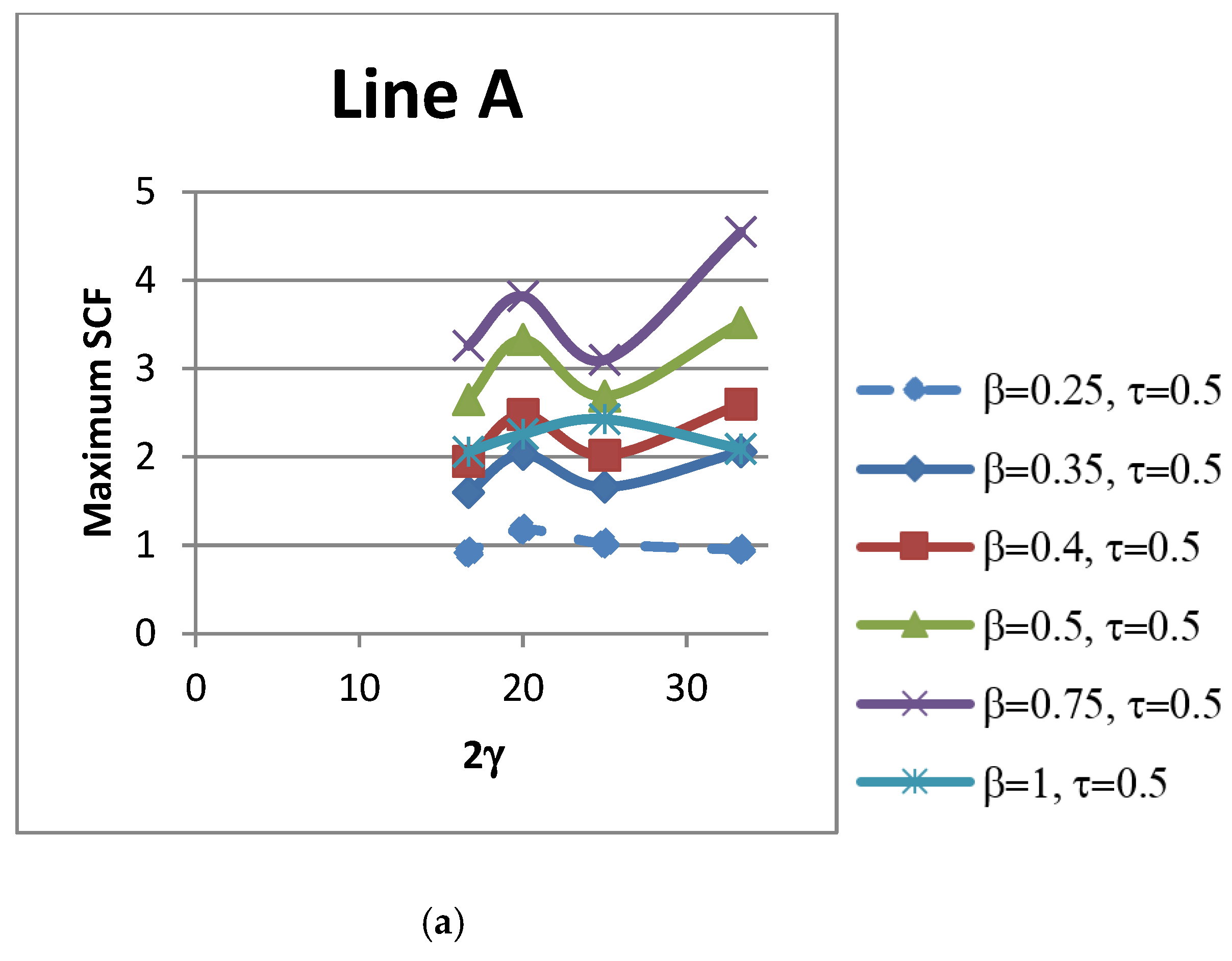
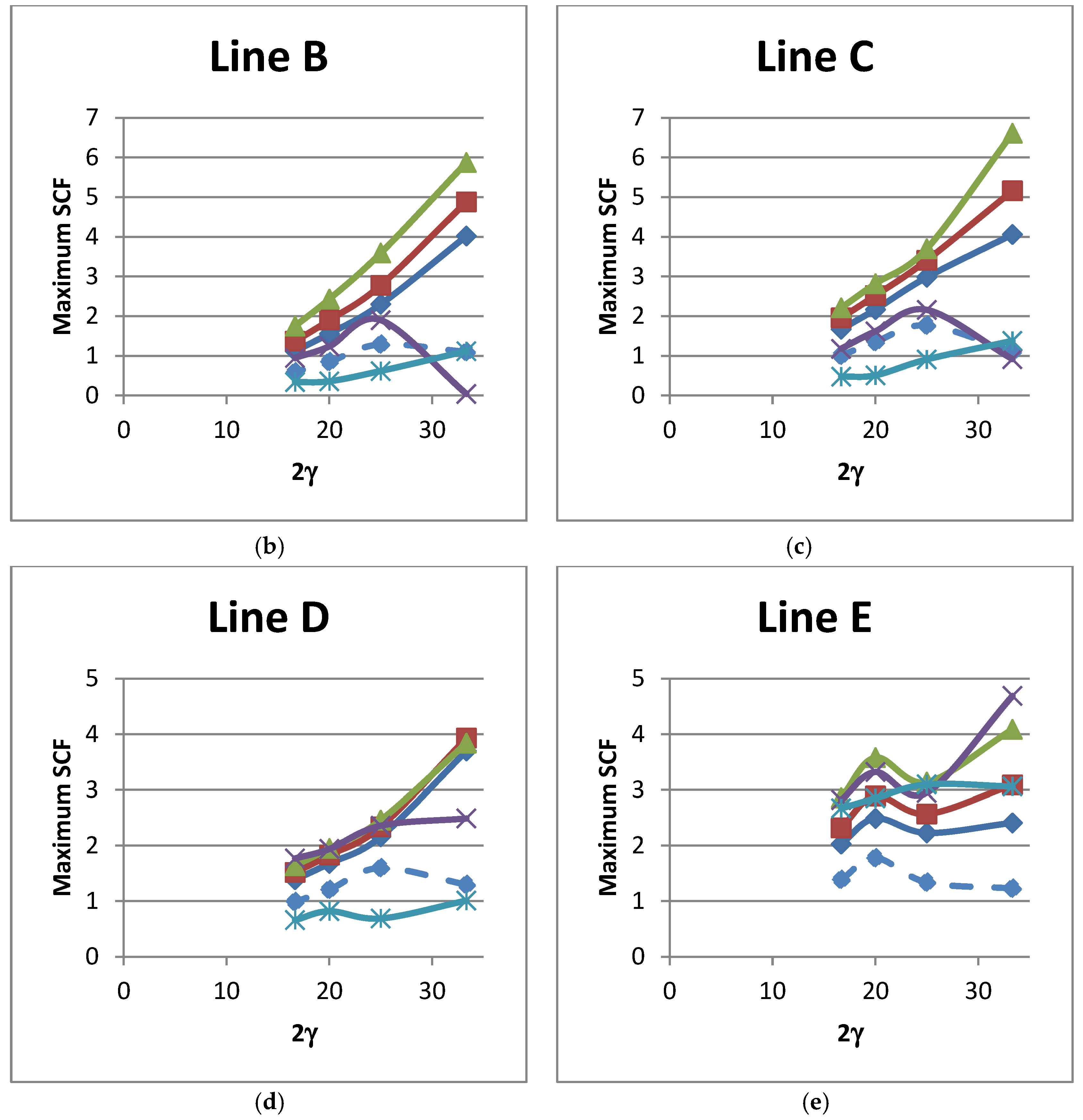
4.4. Influence of 2γ on SCFs
5. Proposed Design Equations
6. Conclusions
Author Contributions
Funding
Institutional Review Board Statement
Informed Consent Statement
Data Availability Statement
Conflicts of Interest
References
- Mashiri, F.R.; Zhao, X.L. Square hollow section (SHS) T-joints with concrete-filled chords subjected to in-plane fatigue loading in the brace. Thin-Walled Struct. 2010, 48, 150–158. [Google Scholar] [CrossRef]
- Matti, F.N.; Mashiri, F.R. Numerical study on SCFs of empty and concrete-filled SHS-SHS T-joints under in-plane bending. In Proceedings of the 9th International Conference on Advances in Steel Structures, Hong Kong, China, 5–7 December 2018. [Google Scholar]
- Jiang, L.; Liu, Y.; Fam, A. Stress concentration factors in concrete-filled square hollow section joints with perfobond ribs. Eng. Struct. 2019, 181, 165–180. [Google Scholar] [CrossRef]
- Matti, F.N.; Mashiri, F.R. Experimental and numerical studies on SCFs of SHS T-Joints subjected to static out-of-plane bending. Thin-Walled Struct. 2020, 146, 106–453. [Google Scholar] [CrossRef]
- Li, T.; Lie, S.T.; Cong, P. Effect of chord axial stresses on the static strength of cracked tubular T/Y-joints under out-of-plane and in-plane bending. Adv. Struct. Eng. 2019, 22, 1698–1710. [Google Scholar] [CrossRef]
- Zhao, X.L.; Herion, S.; Packer, J.A.; Puthli, R.S.; Sedlacek, G.; Wardenier, J.; Weynand, K.; van Wingerde, A.M.; Yeomans, N.F. Design Guide for Circular and Rectangular Hollow Section Welded Joints under Fatigue Loading; TüV-Verlag: Köln, Germany, 2001. [Google Scholar]
- Matti, F.N.; Mashiri, F.R. Experimental and numerical studies on SCFs of empty SHS-SHS T-joints under in-plane bending. Int. J. Eng. Constr. Comput. 2019, 1, 17–26. [Google Scholar]
- Musa, I.A.; Mashiri, F.R. Parametric study and equations of the maximum SCF for concrete filled steel tubular T-joints under in-plane and out-of-plane bending. Thin-Walled Struct. 2019, 135, 245–268. [Google Scholar] [CrossRef]
- Musa, I.A.; Mashiri, F.R.; Zhu, X.; Tong, L. Experimental stress concentration factor in concrete-filled steel tubular T-joints. J. Constr. Steel Res. 2018, 150, 442–451. [Google Scholar] [CrossRef]
- Amer Al-Khamisi, A.; Mashiri, F.R.; Musa, I.; Zhu, X. Stress concentration factors in circular hollow section T-joints with concrete-filled chords. In Proceedings of the 1st International Conference on Engineering Research and Practice, Dhaka, Bangladesh, 4–5 February 2017. [Google Scholar]
- Jamari, J.; Ammarullah, M.I.; Santoso, G.; Sugiharto, S.; Supriyono, T.; Prakoso, A.T.; Basri, H.; van der Heide, E. Computational Contact Pressure Prediction of CoCrMo, SS 316L and Ti6Al4V Femoral Head against UHMWPE Acetabular Cup under Gait Cycle. J. Funct. Biomater. 2022, 13, 64. [Google Scholar] [CrossRef] [PubMed]
- AS 4100-1998; Steel structures. Australian Building Codes Board: Canberra, ACT, Australia, 1998.
- AS 1012.9-2014; Methods of Testing Concrete—Compressive Strength Tests—Concrete, Mortar and Grout Specimens. Australian Building Codes Board: Canberra, ACT, Australia, 2014.
- Ko, Y.; Bathe, K.J. A new 8-node element for analysis of three-dimensional solids. Comput. Struct. 2018, 202, 85–104. [Google Scholar] [CrossRef]
- BussLER, M.L.; Ramesh, A. The eight-node hexahedral element in FEA of part designs. Foundry Manag. Technol. 1993, 121, 26–28. [Google Scholar]
- Shao, Y.B. Proposed equations of stress concentration factor (SCF) for gap tubular K-joints subjected to bending load. Int. J. Space Struct. 2004, 19, 137–147. [Google Scholar] [CrossRef]
- Sonsino, C.M. Effect of residual stresses on the fatigue behaviour of welded joints depending on loading conditions and weld geometry. Int. J. Fatigue 2009, 31, 88–101. [Google Scholar] [CrossRef]
- Chen, Y.; Wan, J.; Hu, K.; Yang, J.; Chen, X. Stress concentration factors of circular chord and square braces K-joints under axial loading. Thin-Walled Struct. 2017, 113, 287–298. [Google Scholar] [CrossRef]
- Ahmadi, H.; Lotfollahi-Yaghin, M.A.; Aminfar, M.H. Geometrical effect on SCF distribution in uni-planar tubular DKT-joints under axial loads. J. Constr. Steel Res. 2011, 67, 1282–1291. [Google Scholar] [CrossRef]
- Musa, I.A.; Mashiri, F.R.; Zhu, X. Parametric study and equation of the maximum SCF for concrete filled steel tubular T-joints under axial tension. Thin-Walled Struct. 2018, 129, 145–156. [Google Scholar] [CrossRef]
- Tong, L.W.; Xu, G.W.; Yang, D.L.; Mashiri, F.R.; Zhao, X.L. Stress concentration factors in CHS-CFSHS T-joints: Experiments. FE analysis and formulae. Eng. Struct. 2017, 15, 406–421. [Google Scholar] [CrossRef]
- Yang, D.; Tong, L. Effects of weld size on stress concentration factors of CHS-CFSHS joints. Frat. Ed. Integrità Strutt. 2018, 12, 45–52. [Google Scholar] [CrossRef]
- van Wingerde, A.M. The fatigue behaviour of T and X joints made of square hollow sections. Heron 1992, 37, 1–182. [Google Scholar]


| Series | Chord | Brace | Non-Dimensional Parameters | ||
|---|---|---|---|---|---|
| S6S1 | 100 × 100 × 4 SHS | 25 × 25 × 3 SHS | 0.25 | 25.00 | 0.75 |
| S5S1 | 100 × 100 × 3 SHS | 25 × 25 × 3 SHS | 0.25 | 33.33 | 1.00 |
| S6S2 | 100 × 100 × 4 SHS | 40 × 40 × 3 SHS | 0.40 | 25.00 | 0.75 |
| S6S3 | 100 × 100 × 4 SHS | 50 × 50 × 3 SHS | 0.50 | 25.00 | 0.75 |
| S6S4 | 100 × 100 × 4 SHS | 75 × 75 × 3 SHS | 0.75 | 25.00 | 0.75 |
| S6S5 | 100 × 100 × 4 SHS | 100 × 100 × 3 SHS | 1.00 | 25.00 | 0.75 |
| S5S5 | 100 × 100 × 3 SHS | 100 × 100 × 3 SHS | 1.00 | 33.33 | 1.00 |
| Extrapolation Points from the Load’s Location (mm) | In-Plane Bending Load (kN) | |||
|---|---|---|---|---|
| 0.50 | 0.71 | 0.92 | 1.21 | |
| Strain (µε) | ||||
| 575 | 0 | 0 | 0 | 0 |
| 375 | 21.35 | 31.85 | 41.28 | 53.08 |
| 250 | 37.60 | 54.89 | 70.60 | 92.09 |
| 125 | 58.41 | 83.17 | 105.34 | 135.96 |
| Nominal strain | 71.83 | 103.11 | 131.24 | 169.84 |
| Test Series | Load, F (N) | Height, H (mm) | Elastic Section Modulus, Z (mm3) | Nominal Strain, (µε) | Young’s Modulus, E (MPa) | σnom.exp = Eε, (MPa) | (MPa) | Ratio |
|---|---|---|---|---|---|---|---|---|
| S6S1 | 193.003 | 575 | 1470 | 325.05 | 222,576.5 | 72.35 | 75.49 | 0.96 |
| 214.451 | 575 | 1470 | 358.85 | 222,576.5 | 79.87 | 83.88 | 0.95 | |
| 238.82 | 575 | 1470 | 394.34 | 222,576.5 | 87.77 | 93.42 | 0.94 | |
| 256.133 | 575 | 1470 | 420.40 | 222,576.5 | 93.57 | 100.19 | 0.93 | |
| S5S1 | 98.647 | 575 | 1470 | 168.61 | 189,604.0 | 31.97 | 38.59 | 0.83 |
| 109.655 | 575 | 1470 | 187.59 | 189,604.0 | 35.57 | 42.89 | 0.83 | |
| 129.065 | 575 | 1470 | 224.31 | 189,604.0 | 42.53 | 50.48 | 0.84 | |
| 139.687 | 575 | 1470 | 265.59 | 189,604.0 | 50.36 | 54.64 | 0.92 | |
| S6S2 | 150.842 | 575 | 4660 | 85.02 | 214,680.5 | 18.25 | 18.61 | 0.98 |
| 195.461 | 575 | 4660 | 109.95 | 214,680.5 | 23.60 | 24.12 | 0.98 | |
| 295.729 | 575 | 4660 | 163.90 | 214,680.5 | 35.19 | 36.49 | 0.96 | |
| 397.128 | 575 | 4660 | 219.79 | 214,680.5 | 47.18 | 49.00 | 0.96 | |
| S6S3 | 192.021 | 575 | 7790 | 63.349 | 215,207.0 | 13.63 | 14.17 | 0.96 |
| 298.084 | 575 | 7790 | 97.66 | 215,207.0 | 21.02 | 22.00 | 0.96 | |
| 394.009 | 575 | 7790 | 129.23 | 215,207.0 | 27.81 | 29.08 | 0.96 | |
| 494.863 | 575 | 7790 | 160.4 | 215,207.0 | 34.52 | 36.53 | 0.95 | |
| S6S4 | 495.543 | 575 | 19,100 | 71.83 | 205,234.0 | 14.74 | 14.92 | 0.99 |
| 714.112 | 575 | 19,100 | 103.11 | 205,234.0 | 21.16 | 21.50 | 0.98 | |
| 915.075 | 575 | 19,100 | 131.24 | 205,234.0 | 26.93 | 27.55 | 0.98 | |
| 1208.042 | 575 | 19,100 | 169.84 | 205,234.0 | 34.86 | 36.37 | 0.96 | |
| S6S5 | 847.142 | 575 | 35,400 | 70.80 | 207,907.0 | 14.72 | 13.76 | 1.07 |
| 2040.564 | 575 | 35,400 | 157.98 | 207,907.0 | 32.85 | 33.14 | 0.99 | |
| 3140.656 | 575 | 35,400 | 245.20 | 207,907.0 | 50.98 | 51.01 | 1.00 | |
| 3585.205 | 575 | 35,400 | 281.57 | 207,907.0 | 58.54 | 58.23 | 1.01 | |
| S5S5 | 1021.493 | 575 | 35,400 | 81.43 | 207,907.0 | 16.93 | 16.59 | 1.02 |
| 1473.567 | 575 | 35,400 | 114.38 | 207,907.0 | 23.78 | 23.94 | 0.99 | |
| 2004.407 | 575 | 35,400 | 152.98 | 207,907.0 | 31.81 | 32.56 | 0.98 | |
| 2500.394 | 575 | 35,400 | 190.08 | 207,907.0 | 39.52 | 40.61 | 0.97 | |
| Average | 0.96 | |||||||
| COV | 0.06 |
| Series | Hot Spot Locations | Load (kN) | HSSN (µε) | Nominal Strain (µε) | SNCF | SNCFSHS | SCFTest |
|---|---|---|---|---|---|---|---|
| S6S1 | Line A | 0.19 | 181.29 | 325.05 | 0.56 | 0.60 | 0.66 |
| 0.21 | 210.59 | 358.85 | 0.59 | ||||
| 0.24 | 243.77 | 394.34 | 0.62 | ||||
| 0.26 | 265.62 | 420.40 | 0.63 | ||||
| Line B | 0.19 | 360.72 | 325.05 | 1.11 | 1.17 | 1.29 | |
| 0.21 | 413.09 | 358.85 | 1.15 | ||||
| 0.24 | 472.59 | 394.34 | 1.20 | ||||
| 0.26 | 515.54 | 420.40 | 1.23 | ||||
| Line C | 0.19 | 633.29 | 325.05 | 1.95 | 1.97 | 2.17 | |
| 0.21 | 703.03 | 358.85 | 1.96 | ||||
| 0.24 | 781.15 | 394.34 | 1.98 | ||||
| 0.26 | 835.23 | 420.40 | 1.99 | ||||
| Line D | 0.19 | 717.1 | 325.05 | 2.21 | 2.18 | 2.39 | |
| 0.21 | 782.54 | 358.85 | 2.18 | ||||
| 0.24 | 853.59 | 394.34 | 2.16 | ||||
| 0.26 | 903.73 | 420.40 | 2.15 | ||||
| Line E | 0.19 | 596.90 | 325.05 | 1.84 | 1.82 | 2.00 | |
| 0.21 | 652.27 | 358.85 | 1.82 | ||||
| 0.24 | 713.26 | 394.34 | 1.81 | ||||
| 0.26 | 756.48 | 420.40 | 1.80 | ||||
| S5S1 | Line A | 0.10 | 147.89 | 168.61 | 0.88 | 0.88 | 0.97 |
| 0.11 | 166.99 | 187.59 | 0.89 | ||||
| 0.13 | 205.93 | 224.31 | 0.92 | ||||
| 0.14 | 226.10 | 265.59 | 0.85 | ||||
| Line B | 0.10 | 197.44 | 168.61 | 1.17 | 1.23 | 1.35 | |
| 0.11 | 229.15 | 187.59 | 1.22 | ||||
| 0.13 | 289.46 | 224.31 | 1.29 | ||||
| 0.14 | 324.06 | 265.59 | 1.22 | ||||
| Line C | 0.10 | 579.74 | 168.61 | 3.44 | 3.46 | 3.81 | |
| 0.11 | 657.33 | 187.59 | 3.50 | ||||
| 0.13 | 803.35 | 224.31 | 3.58 | ||||
| 0.14 | 881.63 | 265.59 | 3.32 | ||||
| Line D | 0.10 | 542.85 | 168.61 | 3.22 | 3.09 | 3.40 | |
| 0.11 | 598.07 | 187.59 | 3.19 | ||||
| 0.13 | 701.28 | 224.31 | 3.13 | ||||
| 0.14 | 753.93 | 265.59 | 2.84 | ||||
| Line E | 0.10 | 218.30 | 168.61 | 1.29 | 1.24 | 1.36 | |
| 0.11 | 239.16 | 187.59 | 1.27 | ||||
| 0.13 | 280.99 | 224.31 | 1.25 | ||||
| 0.14 | 301.75 | 265.59 | 1.14 | ||||
| S6S2 | Line A | 0.15 | 236.00 | 85.02 | 2.78 | 2.82 | 3.11 |
| 0.20 | 305.72 | 109.95 | 2.78 | ||||
| 0.30 | 466.53 | 163.90 | 2.85 | ||||
| 0.40 | 635.96 | 219.79 | 2.89 | ||||
| Line B | 0.15 | 288.42 | 85.02 | 3.39 | 3.50 | 3.85 | |
| 0.20 | 376.60 | 109.95 | 3.43 | ||||
| 0.30 | 582.69 | 163.90 | 3.56 | ||||
| 0.40 | 794.84 | 219.79 | 3.62 | ||||
| Line C | 0.15 | 286.38 | 85.02 | 3.37 | 3.34 | 3.67 | |
| 0.20 | 366.93 | 109.95 | 3.34 | ||||
| 0.30 | 547.33 | 163.90 | 3.34 | ||||
| 0.40 | 726.63 | 219.79 | 3.31 | ||||
| Line D | 0.15 | 235.79 | 85.02 | 2.77 | 2.70 | 2.96 | |
| 0.20 | 299.44 | 109.95 | 2.72 | ||||
| 0.30 | 437.11 | 163.90 | 2.67 | ||||
| 0.40 | 575.04 | 219.79 | 2.62 | ||||
| Line E | 0.15 | 259.57 | 85.02 | 3.05 | 3.02 | 3.32 | |
| 0.20 | 332.01 | 109.95 | 3.02 | ||||
| 0.30 | 493.74 | 163.90 | 3.01 | ||||
| 0.40 | 657.13 | 219.79 | 2.99 | ||||
| S6S3 | Line A | 0.19 | 143.20 | 63.35 | 2.26 | 2.75 | 3.02 |
| 0.30 | 265.00 | 97.66 | 2.71 | ||||
| 0.39 | 378.47 | 129.23 | 2.93 | ||||
| 0.49 | 495.32 | 160.40 | 3.09 | ||||
| Line B | 0.19 | 135.02 | 63.35 | 2.13 | 2.75 | 3.03 | |
| 0.30 | 263.59 | 97.66 | 2.70 | ||||
| 0.39 | 384.87 | 129.23 | 2.98 | ||||
| 0.49 | 514.40 | 160.40 | 3.21 | ||||
| Line C | 0.19 | 181.21 | 63.35 | 2.86 | 3.29 | 3.62 | |
| 0.30 | 321.17 | 97.66 | 3.29 | ||||
| 0.39 | 444.86 | 129.23 | 3.44 | ||||
| 0.49 | 574.99 | 160.40 | 3.58 | ||||
| Line D | 0.19 | 146.27 | 63.35 | 2.31 | 2.40 | 2.64 | |
| 0.30 | 235.30 | 97.66 | 2.41 | ||||
| 0.39 | 313.26 | 129.23 | 2.42 | ||||
| 0.49 | 394.08 | 160.40 | 2.46 | ||||
| Line E | 0.19 | 194.77 | 63.35 | 3.07 | 2.98 | 3.28 | |
| 0.30 | 292.58 | 97.66 | 3.00 | ||||
| 0.39 | 379.70 | 129.23 | 2.94 | ||||
| 0.49 | 469.41 | 160.40 | 2.93 | ||||
| S6S4 | Line A | 0.50 | 305.66 | 71.83 | 4.26 | 4.20 | 4.62 |
| 0.71 | 433.90 | 103.11 | 4.21 | ||||
| 0.92 | 546.25 | 131.24 | 4.16 | ||||
| 1.21 | 707.35 | 169.84 | 4.16 | ||||
| Line B | 0.50 | 114.60 | 71.83 | 1.60 | 1.64 | 1.80 | |
| 0.71 | 166.95 | 103.11 | 1.62 | ||||
| 0.92 | 216.70 | 131.24 | 1.65 | ||||
| 1.21 | 286.61 | 169.84 | 1.69 | ||||
| Line C | 0.50 | 312.58 | 71.83 | 4.35 | 4.15 | 4.57 | |
| 0.71 | 432.08 | 103.11 | 4.19 | ||||
| 0.92 | 535.78 | 131.24 | 4.08 | ||||
| 1.21 | 675.22 | 169.84 | 3.98 | ||||
| Line D | 0.50 | 123.56 | 71.83 | 1.72 | 1.64 | 1.80 | |
| 0.71 | 170.94 | 103.11 | 1.66 | ||||
| 0.92 | 210.24 | 131.24 | 1.60 | ||||
| 1.21 | 266.28 | 169.84 | 1.57 | ||||
| Line E | 0.50 | 160.33 | 71.83 | 2.23 | 2.21 | 2.43 | |
| 0.71 | 226.15 | 103.11 | 2.19 | ||||
| 0.92 | 287.16 | 131.24 | 2.19 | ||||
| 1.21 | 376.02 | 169.84 | 2.21 | ||||
| S6S5 | Line A | 0.85 | 160.91 | 70.80 | 2.27 | 2.00 | 2.20 |
| 2.04 | 315.98 | 157.98 | 2.00 | ||||
| 3.14 | 462.98 | 245.20 | 1.89 | ||||
| 3.59 | 522.55 | 281.57 | 1.86 | ||||
| Line B | 0.85 | 49.08 | 70.80 | 0.69 | 0.47 | 0.52 | |
| 2.04 | 72.23 | 157.98 | 0.46 | ||||
| 3.14 | 92.48 | 245.20 | 0.38 | ||||
| 3.59 | 103.11 | 281.57 | 0.37 | ||||
| Line C | 0.85 | 67.69 | 70.80 | 0.96 | 0.79 | 0.86 | |
| 2.04 | 123.80 | 157.98 | 0.78 | ||||
| 3.14 | 174.83 | 245.20 | 0.71 | ||||
| 3.59 | 193.81 | 281.57 | 0.69 | ||||
| Line D | 0.85 | 59.96 | 70.80 | 0.85 | 0.76 | 0.84 | |
| 2.04 | 118.29 | 157.98 | 0.75 | ||||
| 3.14 | 179.67 | 245.20 | 0.73 | ||||
| 3.59 | 203.50 | 281.57 | 0.72 | ||||
| Line E | 0.85 | 209.33 | 70.80 | 2.96 | 2.95 | 3.24 | |
| 2.04 | 468.46 | 157.98 | 2.97 | ||||
| 3.14 | 719.99 | 245.20 | 2.94 | ||||
| 3.59 | 824.00 | 281.57 | 2.93 | ||||
| S5S5 | Line A | 1.02 | 151.38 | 81.43 | 1.86 | 1.96 | 2.16 |
| 1.47 | 224.19 | 114.38 | 1.96 | ||||
| 2.00 | 308.05 | 152.98 | 2.01 | ||||
| 2.50 | 385.17 | 190.08 | 2.03 | ||||
| Line B | 1.02 | 78.22 | 81.43 | 0.96 | 0.87 | 0.96 | |
| 1.47 | 101.00 | 114.38 | 0.88 | ||||
| 2.00 | 128.69 | 152.98 | 0.84 | ||||
| 2.50 | 151.66 | 190.08 | 0.80 | ||||
| Line C | 1.02 | 58.21 | 81.43 | 0.71 | 0.61 | 0.67 | |
| 1.47 | 75.85 | 114.38 | 0.66 | ||||
| 2.00 | 88.31 | 152.98 | 0.58 | ||||
| 2.50 | 93.03 | 190.08 | 0.49 | ||||
| Line D | 1.02 | 38.11 | 81.43 | 0.47 | 0.51 | 0.56 | |
| 1.47 | 58.52 | 114.38 | 0.51 | ||||
| 2.00 | 80.84 | 152.98 | 0.53 | ||||
| 2.50 | 101.63 | 190.08 | 0.53 | ||||
| Line E | 1.02 | 160.07 | 81.43 | 1.97 | 2.14 | 2.36 | |
| 1.47 | 238.58 | 114.38 | 2.09 | ||||
| 2.00 | 329.62 | 152.98 | 2.15 | ||||
| 2.50 | 448.44 | 190.08 | 2.36 |
| Series Name | DB.MID (mm) | σB.MID (MPa) | DB.QTR (mm) | σB.QTR (MPa) | DB.END (mm) | σnom.FEA Numerical (FEA) (MPa) | σnom.BT Beam Theory (MPa) | Ratio |
|---|---|---|---|---|---|---|---|---|
| S6S1 | 250 | 99.39 | 375 | 51.27 | 0 | 195.62 | 208.16 | 1.06 |
| S5S1 | 250 | 99.39 | 375 | 51.27 | 0 | 195.62 | 208.16 | 1.06 |
| S6S2 | 250 | 32.10 | 375 | 16.56 | 0 | 63.19 | 65.67 | 1.04 |
| S6S3 | 250 | 19.36 | 375 | 9.99 | 0 | 38.11 | 39.28 | 1.03 |
| S6S4 | 250 | 7.97 | 375 | 4.11 | 0 | 15.70 | 16.02 | 1.02 |
| S6S5 | 250 | 4.32 | 375 | 2.23 | 0 | 8.51 | 8.64 | 1.02 |
| S5S5 | 250 | 4.32 | 375 | 2.23 | 0 | 8.51 | 8.64 | 1.02 |
| Average | 1.04 | |||||||
| COV | 0.02 |
| Series | Hot Spot Locations | Load (kN) | Hot Spot Stress (MPa) | Nominal Stress (MPa) | SCFFEA |
|---|---|---|---|---|---|
| S6S1 | Line A | 0.6 | 223.14 | 195.62 | 1.14 |
| Line B | 300.91 | 195.62 | 1.54 | ||
| Line C | 440.38 | 195.62 | 2.25 | ||
| Line D | 393.94 | 195.62 | 2.01 | ||
| Line E | 336.25 | 195.62 | 1.72 | ||
| S5S1 | Line A | 0.6 | 264.40 | 195.62 | 1.35 |
| Line B | 365.44 | 195.62 | 1.87 | ||
| Line C | 372.70 | 195.62 | 1.91 | ||
| Line D | 445.60 | 195.62 | 2.28 | ||
| Line E | 356.02 | 195.62 | 1.82 | ||
| S6S2 | Line A | 0.6 | 160.18 | 63.19 | 2.53 |
| Line B | 232.19 | 63.19 | 3.67 | ||
| Line C | 290.24 | 63.19 | 4.59 | ||
| Line D | 192.33 | 63.19 | 3.04 | ||
| Line E | 181.97 | 63.19 | 2.88 | ||
| S6S3 | Line A | 0.6 | 132.17 | 38.11 | 3.47 |
| Line B | 188.55 | 38.11 | 4.95 | ||
| Line C | 188.74 | 38.11 | 4.95 | ||
| Line D | 123.95 | 38.11 | 3.25 | ||
| Line E | 134.57 | 38.11 | 3.53 | ||
| S6S4 | Line A | 0.6 | 63.24 | 15.69 | 4.03 |
| Line B | 39.85 | 15.69 | 2.54 | ||
| Line C | 37.88 | 15.69 | 2.41 | ||
| Line D | 51.63 | 15.69 | 3.29 | ||
| Line E | 48.61 | 15.69 | 3.10 | ||
| S6S5 | Line A | 0.6 | 24.71 | 8.51 | 2.91 |
| Line B | 13.13 | 8.51 | 1.54 | ||
| Line C | 19.26 | 8.51 | 2.26 | ||
| Line D | 9.71 | 8.51 | 1.14 | ||
| Line E | 34.30 | 8.51 | 4.03 | ||
| S5S5 | Line A | 0.6 | 24.10 | 8.51 | 2.83 |
| Line B | 18.23 | 8.51 | 2.14 | ||
| Line C | 22.71 | 8.51 | 2.67 | ||
| Line D | 18.53 | 8.51 | 2.18 | ||
| Line E | 36.12 | 8.51 | 4.25 |
| Series Name | Non-Dimensional Parameters | Empty/Concrete | Experimental SCF (Quadratic) | Peak SCF | Reduction % in Peak SCF | ||||||
|---|---|---|---|---|---|---|---|---|---|---|---|
| β | 2γ | τ | Chord | Brace | |||||||
| B | C | D | A | E | |||||||
| S6S1 | 0.25 | 25 | 0.75 | Empty | 2.07 | 2.58 | 2.70 | 0.28 | 2.22 | 2.70 | 11.48 |
| Concrete | 1.29 | 2.17 | 2.39 | 0.66 | 2.00 | 2.39 | |||||
| S5S1 | 0.25 | 33.33 | 1.00 | Empty | 1.37 | 4.27 | 3.55 | 0.90 | 2.37 | 4.27 | 10.77 |
| Concrete | 1.35 | 3.81 | 3.40 | 0.97 | 1.36 | 3.81 | |||||
| S6S2 | 0.40 | 25 | 0.75 | Empty | 3.38 | 4.65 | 5.38 | 2.41 | 3.06 | 5.38 | 28.44 |
| Concrete | 3.85 | 3.67 | 2.96 | 3.11 | 3.32 | 3.85 | |||||
| S6S3 | 0.50 | 25 | 0.75 | Empty | 4.45 | 5.04 | 5.76 | 3.57 | 3.54 | 5.76 | 37.15 |
| Concrete | 3.03 | 3.62 | 2.64 | 3.02 | 3.28 | 3.62 | |||||
| S6S4 | 0.75 | 25 | 0.75 | Empty | 1.19 | 4.90 | 2.80 | 5.82 | 3.07 | 5.82 | 20.62 |
| Concrete | 1.80 | 4.57 | 1.80 | 4.62 | 2.43 | 4.62 | |||||
| S6S5 | 1.00 | 25 | 0.75 | Empty | 1.12 | 1.25 | 1.16 | 2.34 | 3.66 | 3.66 | 11.48 |
| Concrete | 0.52 | 0.86 | 0.84 | 2.20 | 3.24 | 3.24 | |||||
| S5S5 | 1.00 | 33.33 | 1.00 | Empty | 3.08 | 2.29 | 1.49 | 3.64 | 2.90 | 3.64 | 35.16 |
| Concrete | 0.96 | 0.67 | 0.56 | 2.16 | 2.36 | 2.36 | |||||
| Mean | 22.16 | ||||||||||
| Series Name | Stress Concentration Factor (SCF) | Reduction % in Peak SCF | |||||||||
|---|---|---|---|---|---|---|---|---|---|---|---|
| Empty SHS T-Joints Matti and Mashiri [7] | Concrete-Filled SHS T-Joints | ||||||||||
| B | C | D | A | E | B | C | D | A | E | ||
| S6S1 | 1.16 | 2.35 | 2.28 | 0.92 | 1.82 | 1.54 | 2.25 | 2.01 | 1.14 | 1.72 | 4.26 |
| S5S1 | 2.18 | 2.50 | 3.11 | 1.03 | 1.98 | 1.87 | 1.91 | 2.28 | 1.35 | 1.82 | 26.69 |
| S6S2 | 3.34 | 5.43 | 4.02 | 2.37 | 3.17 | 3.67 | 4.59 | 3.04 | 2.53 | 2.88 | 15.47 |
| S6S3 | 5.00 | 6.02 | 4.55 | 3.61 | 4.03 | 4.95 | 4.95 | 3.25 | 3.47 | 3.53 | 17.77 |
| S6S4 | 7.15 | 5.06 | 4.92 | 5.24 | 3.89 | 2.54 | 2.41 | 3.29 | 4.03 | 3.10 | 43.64 |
| S6S5 | 1.55 | 2.31 | 1.23 | 3.82 | 4.58 | 1.54 | 2.26 | 1.14 | 2.91 | 4.03 | 12.01 |
| S5S5 | 2.30 | 3.24 | 2.19 | 4.29 | 4.85 | 2.14 | 2.67 | 2.18 | 2.83 | 4.25 | 12.37 |
| Average | 18.89 | ||||||||||
| Series Name | Non-Dimensional Parameters | FEA/ Test | SCF (Quadratic) | Maximum SCF | Ratio of Maximum SCFs | ||||||
|---|---|---|---|---|---|---|---|---|---|---|---|
| Chord | Brace | ||||||||||
| B | C | D | A | E | |||||||
| S6S1 | 0.25 | 25 | 0.75 | FEA | 1.54 | 2.25 | 2.01 | 1.14 | 1.72 | 2.25 | 0.94 |
| Test | 1.29 | 2.17 | 2.39 | 0.66 | 2.00 | 2.39 | |||||
| S5S1 | 0.25 | 33.33 | 1.00 | FEA | 1.87 | 1.91 | 2.28 | 1.35 | 1.82 | 2.28 | 0.60 |
| Test | 1.35 | 3.81 | 3.40 | 0.97 | 1.36 | 3.81 | |||||
| S6S2 | 0.40 | 25 | 0.75 | FEA | 3.67 | 4.59 | 3.04 | 2.53 | 2.88 | 4.59 | 1.19 |
| Test | 3.85 | 3.67 | 2.96 | 3.11 | 3.32 | 3.85 | |||||
| S6S3 | 0.50 | 25 | 0.75 | FEA | 4.95 | 4.95 | 3.25 | 3.47 | 3.53 | 4.95 | 1.37 |
| Test | 3.03 | 3.62 | 2.64 | 3.02 | 3.28 | 3.62 | |||||
| S6S4 | 0.75 | 25 | 0.75 | FEA | 2.54 | 2.41 | 3.29 | 4.03 | 3.10 | 4.03 | 0.87 |
| Test | 1.80 | 4.57 | 1.80 | 4.62 | 2.43 | 4.62 | |||||
| S6S5 | 1.00 | 25 | 0.75 | FEA | 1.54 | 2.26 | 1.14 | 2.91 | 4.03 | 4.03 | 1.24 |
| Test | 0.52 | 0.86 | 0.84 | 2.20 | 3.24 | 3.24 | |||||
| S5S5 | 1.00 | 33.33 | 1.00 | FEA | 2.14 | 2.67 | 2.18 | 2.83 | 4.25 | 4.25 | 1.80 |
| Test | 0.96 | 0.67 | 0.56 | 2.16 | 2.36 | 2.36 | |||||
| Average | 1.15 | ||||||||||
| Series Name | SHS Chord | SHS Brace | Non-Dimensional Parameters | SCFCFSHS.FE | ||||||
|---|---|---|---|---|---|---|---|---|---|---|
| A | B | C | D | E | ||||||
| S21S1 | SHS | SHS | 0.25 | 33.33 | 1.0 | 1.35 | 1.87 | 1.91 | 2.28 | 1.82 |
| S21S2 | SHS | SHS | 0.25 | 33.33 | 0.83 | 1.59 | 1.59 | 1.65 | 1.95 | 1.98 |
| S21S3 | SHS | SHS | 0.25 | 33.33 | 0.67 | 1.32 | 1.33 | 1.35 | 1.58 | 1.39 |
| S21S4 | SHS | SHS | 0.25 | 33.33 | 0.53 | 0.95 | 1.10 | 1.11 | 1.30 | 1.23 |
| S21S5 | SHS | SHS | 0.35 | 33.33 | 1.0 | 2.36 | 6.17 | 6.40 | 5.45 | 2.77 |
| S21S6 | SHS | SHS | 0.35 | 33.33 | 0.83 | 2.66 | 5.62 | 5.70 | 4.96 | 3.21 |
| S21S7 | SHS | SHS | 0.35 | 33.33 | 0.67 | 1.87 | 4.80 | 4.85 | 4.32 | 2.49 |
| S21S8 | SHS | SHS | 0.35 | 33.33 | 0.53 | 2.06 | 4.02 | 4.06 | 3.70 | 2.41 |
| S21S9 | SHS | SHS | 0.4 | 33.33 | 1.0 | 2.95 | 7.73 | 8.25 | 5.73 | 3.25 |
| S21S10 | SHS | SHS | 0.4 | 33.33 | 0.83 | 3.34 | 6.86 | 7.31 | 5.22 | 3.79 |
| S21S11 | SHS | SHS | 0.4 | 33.33 | 0.67 | 2.31 | 5.83 | 6.17 | 4.57 | 2.94 |
| S21S12 | SHS | SHS | 0.4 | 33.33 | 0.53 | 2.60 | 4.88 | 5.16 | 3.93 | 3.09 |
| S21S13 | SHS | SHS | 0.5 | 33.33 | 1.0 | 4.12 | 9.29 | 10.59 | 5.73 | 4.00 |
| S21S14 | SHS | SHS | 0.5 | 33.33 | 0.83 | 4.59 | 8.23 | 9.39 | 5.19 | 4.71 |
| S21S15 | SHS | SHS | 0.5 | 33.33 | 0.67 | 3.14 | 6.99 | 7.93 | 4.50 | 3.62 |
| S21S16 | SHS | SHS | 0.5 | 33.33 | 0.53 | 3.52 | 5.87 | 6.61 | 3.84 | 4.09 |
| S21S17 | SHS | SHS | 0.75 | 33.33 | 1.0 | 5.98 | 0.11 | 1.06 | 3.87 | 4.47 |
| S21S18 | SHS | SHS | 0.75 | 33.33 | 0.83 | 6.37 | 0.08 | 1.06 | 3.61 | 5.29 |
| S21S19 | SHS | SHS | 0.75 | 33.33 | 0.67 | 4.26 | 0.06 | 1.01 | 3.13 | 4.14 |
| S21S20 | SHS | SHS | 0.75 | 33.33 | 0.53 | 4.55 | 0.04 | 0.92 | 2.49 | 4.69 |
| S21S21 | SHS | SHS | 1 | 33.33 | 1.0 | 2.83 | 2.14 | 2.67 | 2.18 | 4.25 |
| S21S22 | SHS | SHS | 1 | 33.33 | 0.83 | 2.90 | 1.79 | 2.21 | 1.76 | 4.26 |
| S21S23 | SHS | SHS | 1 | 33.33 | 0.67 | 2.05 | 1.41 | 1.73 | 1.30 | 3.08 |
| S21S24 | SHS | SHS | 1 | 33.33 | 0.53 | 2.09 | 1.12 | 1.38 | 1.01 | 3.06 |
| S25S1 | SHS | SHS | 0.25 | 25 | 0.75 | 1.14 | 1.54 | 2.25 | 2.01 | 1.72 |
| S25S2 | SHS | SHS | 0.25 | 25 | 0.63 | 1.34 | 1.44 | 2.06 | 1.84 | 1.92 |
| S25S2 | SHS | SHS | 0.25 | 25 | 0.5 | 1.02 | 1.29 | 1.77 | 1.60 | 1.34 |
| S25S4 | SHS | SHS | 0.25 | 25 | 0.4 | 1.03 | 1.11 | 1.51 | 1.39 | 1.28 |
| S25S5 | SHS | SHS | 0.35 | 25 | 0.75 | 2.05 | 2.98 | 3.97 | 2.78 | 2.49 |
| S25S6 | SHS | SHS | 0.35 | 25 | 0.63 | 2.33 | 2.67 | 3.52 | 2.50 | 2.83 |
| S25S7 | SHS | SHS | 0.35 | 25 | 0.5 | 1.66 | 2.30 | 2.98 | 2.16 | 2.23 |
| S25S8 | SHS | SHS | 0.35 | 25 | 0.4 | 1.87 | 1.94 | 2.48 | 1.84 | 2.33 |
| S25S9 | SHS | SHS | 0.4 | 25 | 0.75 | 2.53 | 3.67 | 4.59 | 3.04 | 2.88 |
| S25S10 | SHS | SHS | 0.4 | 25 | 0.63 | 2.87 | 3.26 | 4.05 | 2.73 | 3.30 |
| S25S11 | SHS | SHS | 0.4 | 25 | 0.5 | 2.02 | 2.78 | 3.41 | 2.34 | 2.57 |
| S25S12 | SHS | SHS | 0.4 | 25 | 0.4 | 2.26 | 2.32 | 2.84 | 1.98 | 2.79 |
| S25S13 | SHS | SHS | 0.5 | 25 | 0.75 | 3.47 | 4.95 | 4.95 | 3.25 | 3.53 |
| S25S14 | SHS | SHS | 0.5 | 25 | 0.63 | 3.85 | 4.31 | 4.39 | 2.89 | 4.06 |
| S25S15 | SHS | SHS | 0.5 | 25 | 0.5 | 2.69 | 3.59 | 3.70 | 2.46 | 3.14 |
| S25S16 | SHS | SHS | 0.5 | 25 | 0.4 | 2.96 | 2.93 | 3.05 | 2.05 | 3.45 |
| S25S17 | SHS | SHS | 0.75 | 25 | 0.75 | 4.03 | 2.54 | 2.41 | 3.29 | 3.10 |
| S25S18 | SHS | SHS | 0.75 | 25 | 0.63 | 4.28 | 2.22 | 2.47 | 2.88 | 3.54 |
| S25S19 | SHS | SHS | 0.75 | 25 | 0.5 | 3.10 | 1.90 | 2.16 | 2.36 | 2.95 |
| S25S20 | SHS | SHS | 0.75 | 25 | 0.4 | 3.27 | 1.60 | 1.79 | 1.89 | 3.26 |
| S25S21 | SHS | SHS | 1 | 25 | 0.75 | 2.91 | 1.54 | 2.26 | 1.14 | 4.03 |
| S25S22 | SHS | SHS | 1 | 25 | 0.63 | 3.51 | 0.83 | 1.22 | 0.91 | 4.33 |
| S25S23 | SHS | SHS | 1 | 25 | 0.5 | 2.43 | 0.62 | 0.91 | 0.69 | 3.10 |
| S25S24 | SHS | SHS | 1 | 25 | 0.4 | 2.42 | 0.44 | 0.65 | 0.52 | 3.06 |
| S26S2 | SHS | SHS | 0.25 | 20 | 0.5 | 1.18 | 0.85 | 1.35 | 1.21 | 1.78 |
| S26S6 | SHS | SHS | 0.35 | 20 | 0.5 | 2.03 | 1.56 | 2.17 | 1.68 | 2.49 |
| S26S10 | SHS | SHS | 0.4 | 20 | 0.5 | 2.48 | 1.90 | 2.52 | 1.83 | 2.89 |
| S26S14 | SHS | SHS | 0.5 | 20 | 0.5 | 3.33 | 2.43 | 2.82 | 1.95 | 3.58 |
| S26S18 | SHS | SHS | 0.75 | 20 | 0.5 | 3.82 | 1.24 | 1.62 | 1.94 | 3.32 |
| S26S22 | SHS | SHS | 1 | 20 | 0.5 | 2.26 | 0.36 | 0.51 | 0.82 | 2.85 |
| S27S1 | SHS | SHS | 0.25 | 16.67 | 0.5 | 0.92 | 0.59 | 1.01 | 0.99 | 1.39 |
| S27S5 | SHS | SHS | 0.35 | 16.67 | 0.5 | 1.60 | 1.12 | 1.67 | 1.39 | 2.03 |
| S27S9 | SHS | SHS | 0.4 | 16.67 | 0.5 | 1.95 | 1.37 | 1.96 | 1.52 | 2.32 |
| S27S13 | SHS | SHS | 0.5 | 16.67 | 0.5 | 2.65 | 1.75 | 2.21 | 1.64 | 2.86 |
| S27S17 | SHS | SHS | 0.75 | 16.67 | 0.5 | 3.26 | 0.95 | 1.18 | 1.77 | 2.82 |
| S27S21 | SHS | SHS | 1 | 16.67 | 0.5 | 2.06 | 0.34 | 0.48 | 0.66 | 2.67 |
| β | 2γ = 33.33 τ = 1 | 2γ = 33.33 τ = 0.8 | 2γ = 33.33 τ = 0.67 | 2γ = 33.33 τ = 0.5 | 2γ = 20 τ = 0.5 | 2γ = 16.67 τ = 0.5 | 2γ = 25 τ = 0.75 | 2γ = 25 τ = 0.63 | 2γ = 25 τ = 0.5 | 2γ = 25 τ = 0.4 |
|---|---|---|---|---|---|---|---|---|---|---|
| 0.25 | 2.28 | 1.98 | 1.58 | 1.3 | 1.78 | 1.39 | 2.25 | 2.06 | 1.77 | 1.51 |
| 0.35 | 6.4 | 5.7 | 4.85 | 4.06 | 2.49 | 2.03 | 3.97 | 3.52 | 2.98 | 2.48 |
| 0.4 | 8.25 | 7.31 | 6.17 | 5.16 | 2.89 | 2.32 | 4.59 | 4.05 | 3.41 | 2.84 |
| 0.5 | 10.59 | 9.39 | 7.93 | 6.61 | 3.58 | 2.86 | 4.95 | 4.39 | 3.7 | 3.45 |
| 0.75 | 5.98 | 6.37 | 4.26 | 4.69 | 3.82 | 3.26 | 4.03 | 4.28 | 3.1 | 3.27 |
| 1 | 4.25 | 4.26 | 3.08 | 3.06 | 2.85 | 2.67 | 4.03 | 4.33 | 3.1 | 3.06 |
| τ = 0.53 | τ = 0.67 | τ = 0.83 | τ = 1 | |
| β = 0.25, 2γ = 33.33 | 1.3 | 1.58 | 1.98 | 2.28 |
| β = 0.35, 2γ = 33.33 | 4.06 | 4.85 | 5.7 | 6.4 |
| β = 0.4, 2γ = 33.33 | 5.16 | 6.17 | 7.31 | 8.25 |
| β = 0.5, 2γ = 33.33 | 6.61 | 7.93 | 9.39 | 10.59 |
| β = 0.75, 2γ = 33.33 | 4.69 | 4.26 | 6.37 | 5.98 |
| β = 1, 2γ = 33.33 | 3.06 | 3.08 | 4.26 | 4.25 |
| τ = 0.40 | τ = 0.50 | τ = 0.63 | τ = 0.75 | |
| β = 0.25, 2γ = 25 | 1.51 | 1.77 | 2.06 | 2.25 |
| β = 0.35, 2γ = 25 | 2.48 | 2.98 | 3.52 | 3.97 |
| β = 0.4, 2γ = 25 | 2.84 | 3.41 | 4.05 | 4.59 |
| β = 0.5, 2γ = 25 | 3.45 | 3.7 | 4.39 | 4.95 |
| β = 0.75, 2γ = 25 | 3.27 | 3.1 | 4.28 | 4.03 |
| β = 1, 2γ = 25 | 3.06 | 3.1 | 4.33 | 4.03 |
| 2γ | β = 0.25 τ = 0.5 | β = 0.35 τ = 0.5 | β = 0.4 τ = 0.5 | β = 0.5 τ = 0.5 | β = 0.75 τ = 0.5 | β = 1 τ = 0.5 |
|---|---|---|---|---|---|---|
| 33.33 | 1.3 | 4.06 | 5.16 | 6.61 | 4.69 | 3.06 |
| 25 | 1.77 | 2.98 | 3.41 | 3.7 | 3.1 | 3.1 |
| 20 | 1.78 | 2.49 | 2.89 | 3.58 | 3.82 | 2.85 |
| 16.67 | 1.39 | 2.03 | 2.32 | 2.86 | 3.26 | 2.67 |
| Constants | Line A | Line B | Line C | Line D | Line E | Peak SCF |
|---|---|---|---|---|---|---|
| a | 5.683849 | 0.006668 | 0.069071 | 0.067958 | 4.584246 | 0.233257 |
| b | −11.161296 | −0.014833 | −0.157049 | −0.179585 | −9.546303 | −0.467340 |
| c | 5.662125 | 0.009966 | 0.101481 | 0.139751 | 5.075972 | 0.258524 |
| d | −0.004096 | −0.000034 | −0.000232 | −0.000231 | −0.002281 | −0.000598 |
| e | −0.856986 | 0.465188 | −0.051707 | 0.027163 | −0.630846 | 0.096247 |
| f | 2.760551 | 7.327060 | 6.575175 | 6.553876 | 2.298098 | 3.977695 |
| g | −0.737920 | −5.509643 | −4.793702 | −5.285170 | −0.338629 | −2.104667 |
| h | 0.455557 | 0.736167 | 0.750481 | 0.682011 | 0.246473 | 0.700215 |
| Series Name | Non-Dimensional Parameters | SCFFE of Concrete-Filled T-Joints under In-Plane Bending | Peak SCF | ||||||||
|---|---|---|---|---|---|---|---|---|---|---|---|
| β | 2γ | τ | A | B | C | D | E | FE | Predicted | ||
| S21S1 | 0.25 | 33.33 | 1 | 1.35 | 1.87 | 1.91 | 2.28 | 1.82 | 2.28 | 3.25 | 1.43 |
| S21S2 | 0.25 | 33.33 | 0.83 | 1.59 | 1.59 | 1.65 | 1.95 | 1.98 | 1.98 | 2.86 | 1.44 |
| S21S3 | 0.25 | 33.33 | 0.67 | 1.32 | 1.33 | 1.35 | 1.58 | 1.39 | 1.58 | 2.46 | 1.56 |
| S21S4 | 0.25 | 33.33 | 0.53 | 0.95 | 1.1 | 1.11 | 1.3 | 1.23 | 1.3 | 2.09 | 1.60 |
| S21S5 | 0.35 | 33.33 | 1 | 2.36 | 6.17 | 6.4 | 5.45 | 2.77 | 6.4 | 6.09 | 0.95 |
| S21S6 | 0.35 | 33.33 | 0.83 | 2.66 | 5.62 | 5.7 | 4.96 | 3.21 | 5.7 | 5.35 | 0.94 |
| S21S7 | 0.35 | 33.33 | 0.67 | 1.87 | 4.8 | 4.85 | 4.32 | 2.49 | 4.85 | 4.60 | 0.95 |
| S21S8 | 0.35 | 33.33 | 0.53 | 2.06 | 4.02 | 4.06 | 3.7 | 2.41 | 4.06 | 3.91 | 0.96 |
| S21S9 | 0.4 | 33.33 | 1 | 2.95 | 7.73 | 8.25 | 5.73 | 3.25 | 8.25 | 7.72 | 0.94 |
| S21S10 | 0.4 | 33.33 | 0.83 | 3.34 | 6.86 | 7.31 | 5.22 | 3.79 | 7.31 | 6.78 | 0.93 |
| S21S11 | 0.4 | 33.33 | 0.67 | 2.31 | 5.83 | 6.17 | 4.57 | 2.94 | 6.17 | 5.83 | 0.95 |
| S21S12 | 0.4 | 33.33 | 0.53 | 2.6 | 4.88 | 5.16 | 3.93 | 3.09 | 5.16 | 4.95 | 0.96 |
| S21S13 | 0.5 | 33.33 | 1 | 4.12 | 9.29 | 10.59 | 5.73 | 4 | 10.59 | 10.48 | 0.99 |
| S21S14 | 0.5 | 33.33 | 0.83 | 4.59 | 8.23 | 9.39 | 5.19 | 4.71 | 9.39 | 9.20 | 0.98 |
| S21S15 | 0.5 | 33.33 | 0.67 | 3.14 | 6.99 | 7.93 | 4.5 | 3.62 | 7.93 | 7.92 | 1.00 |
| S21S16 | 0.5 | 33.33 | 0.53 | 3.52 | 5.87 | 6.61 | 3.84 | 4.09 | 6.61 | 6.72 | 1.02 |
| S21S17 | 0.75 | 33.33 | 1 | 5.98 | 0.11 | 1.06 | 3.87 | 4.47 | 5.98 | 6.35 | 1.06 |
| S21S18 | 0.75 | 33.33 | 0.83 | 6.37 | 0.08 | 1.06 | 3.61 | 5.29 | 6.37 | 5.57 | 0.87 |
| S21S19 | 0.75 | 33.33 | 0.67 | 4.26 | 0.06 | 1.01 | 3.13 | 4.14 | 4.26 | 4.80 | 1.13 |
| S21S20 | 0.75 | 33.33 | 0.53 | 4.55 | 0.04 | 0.92 | 2.49 | 4.69 | 4.69 | 4.07 | 0.87 |
| S21S21 | 1 | 33.33 | 1 | 2.83 | 2.14 | 2.67 | 2.18 | 4.25 | 4.25 | 4.50 | 1.06 |
| S21S22 | 1 | 33.33 | 0.83 | 2.9 | 1.79 | 2.21 | 1.76 | 4.26 | 4.26 | 3.95 | 0.93 |
| S21S23 | 1 | 33.33 | 0.67 | 2.05 | 1.41 | 1.73 | 1.3 | 3.08 | 3.08 | 3.40 | 1.10 |
| S21S24 | 1 | 33.33 | 0.53 | 2.09 | 1.12 | 1.38 | 1.01 | 3.06 | 3.06 | 2.88 | 0.94 |
| S25S1 | 0.25 | 25 | 0.75 | 1.14 | 1.54 | 2.25 | 2.01 | 1.72 | 2.25 | 2.11 | 0.94 |
| S25S2 | 0.25 | 25 | 0.63 | 1.34 | 1.44 | 2.06 | 1.84 | 1.92 | 2.06 | 1.87 | 0.91 |
| S25S2 | 0.25 | 25 | 0.5 | 1.02 | 1.29 | 1.77 | 1.6 | 1.34 | 1.77 | 1.59 | 0.90 |
| S25S4 | 0.25 | 25 | 0.4 | 1.03 | 1.11 | 1.51 | 1.39 | 1.28 | 1.51 | 1.36 | 0.90 |
| S25S5 | 0.35 | 25 | 0.75 | 2.05 | 2.98 | 3.97 | 2.78 | 2.49 | 3.97 | 3.71 | 0.93 |
| S25S6 | 0.35 | 25 | 0.63 | 2.33 | 2.67 | 3.52 | 2.5 | 2.83 | 3.52 | 3.28 | 0.93 |
| S25S7 | 0.35 | 25 | 0.5 | 1.66 | 2.3 | 2.98 | 2.16 | 2.23 | 2.98 | 2.79 | 0.94 |
| S25S8 | 0.35 | 25 | 0.4 | 1.87 | 1.94 | 2.48 | 1.84 | 2.33 | 2.48 | 2.39 | 0.96 |
| S25S9 | 0.4 | 25 | 0.75 | 2.53 | 3.67 | 4.59 | 3.04 | 2.88 | 4.59 | 4.60 | 1.00 |
| S25S10 | 0.4 | 25 | 0.63 | 2.87 | 3.26 | 4.05 | 2.73 | 3.3 | 4.05 | 4.07 | 1.00 |
| S25S11 | 0.4 | 25 | 0.5 | 2.02 | 2.78 | 3.41 | 2.34 | 2.57 | 3.41 | 3.46 | 1.01 |
| S25S12 | 0.4 | 25 | 0.4 | 2.26 | 2.32 | 2.84 | 1.98 | 2.79 | 2.84 | 2.96 | 1.04 |
| S25S13 | 0.5 | 25 | 0.75 | 3.47 | 4.95 | 4.95 | 3.25 | 3.53 | 4.95 | 6.09 | 1.23 |
| S25S14 | 0.5 | 25 | 0.63 | 3.85 | 4.31 | 4.39 | 2.89 | 4.06 | 4.39 | 5.39 | 1.23 |
| S25S15 | 0.5 | 25 | 0.5 | 2.69 | 3.59 | 3.7 | 2.46 | 3.14 | 3.7 | 4.58 | 1.24 |
| S25S16 | 0.5 | 25 | 0.4 | 2.96 | 2.93 | 3.05 | 2.05 | 3.45 | 3.45 | 3.92 | 1.14 |
| S25S17 | 0.75 | 25 | 0.75 | 4.03 | 2.54 | 2.41 | 3.29 | 3.1 | 4.03 | 4.83 | 1.20 |
| S25S18 | 0.75 | 25 | 0.63 | 4.28 | 2.22 | 2.47 | 2.88 | 3.54 | 4.28 | 4.27 | 1.00 |
| S25S19 | 0.75 | 25 | 0.5 | 3.1 | 1.9 | 2.16 | 2.36 | 2.95 | 3.1 | 3.63 | 1.17 |
| S25S20 | 0.75 | 25 | 0.4 | 3.27 | 1.6 | 1.79 | 1.89 | 3.26 | 3.27 | 3.11 | 0.95 |
| S25S21 | 1 | 25 | 0.75 | 2.91 | 1.54 | 2.26 | 1.14 | 4.03 | 4.03 | 4.39 | 1.09 |
| S25S22 | 1 | 25 | 0.63 | 3.51 | 0.83 | 1.22 | 0.91 | 4.33 | 4.33 | 3.89 | 0.90 |
| S25S23 | 1 | 25 | 0.5 | 2.43 | 0.62 | 0.91 | 0.69 | 3.1 | 3.1 | 3.31 | 1.07 |
| S25S24 | 1 | 25 | 0.4 | 2.42 | 0.44 | 0.65 | 0.52 | 3.06 | 3.06 | 2.83 | 0.92 |
| S26S2 | 0.25 | 20 | 0.5 | 1.18 | 0.85 | 1.35 | 1.21 | 1.78 | 1.78 | 1.31 | 0.74 |
| S26S6 | 0.35 | 20 | 0.5 | 2.03 | 1.56 | 2.17 | 1.68 | 2.49 | 2.49 | 2.20 | 0.88 |
| S26S10 | 0.4 | 20 | 0.5 | 2.48 | 1.9 | 2.52 | 1.83 | 2.89 | 2.89 | 2.66 | 0.92 |
| S26S14 | 0.5 | 20 | 0.5 | 3.33 | 2.43 | 2.82 | 1.95 | 3.58 | 3.58 | 3.43 | 0.96 |
| S26S18 | 0.75 | 20 | 0.5 | 3.82 | 1.24 | 1.62 | 1.94 | 3.32 | 3.82 | 2.92 | 0.76 |
| S26S22 | 1 | 20 | 0.5 | 2.26 | 0.36 | 0.51 | 0.82 | 2.85 | 2.85 | 2.80 | 0.98 |
| S27S1 | 0.25 | 16.67 | 0.5 | 0.92 | 0.59 | 1.01 | 0.99 | 1.39 | 1.39 | 1.12 | 0.81 |
| S27S5 | 0.35 | 16.67 | 0.5 | 1.6 | 1.12 | 1.67 | 1.39 | 2.03 | 2.03 | 1.79 | 0.88 |
| S27S9 | 0.4 | 16.67 | 0.5 | 1.95 | 1.37 | 1.96 | 1.52 | 2.32 | 2.32 | 2.14 | 0.92 |
| S27S13 | 0.5 | 16.67 | 0.5 | 2.65 | 1.75 | 2.21 | 1.64 | 2.86 | 2.86 | 2.68 | 0.94 |
| S27S17 | 0.75 | 16.67 | 0.5 | 3.26 | 0.95 | 1.18 | 1.77 | 2.82 | 3.26 | 2.32 | 0.71 |
| S27S21 | 1 | 16.67 | 0.5 | 2.06 | 0.34 | 0.48 | 0.66 | 2.67 | 2.67 | 2.27 | 0.85 |
| STDEV | 0.17 | ||||||||||
| Mean | 1.01 | ||||||||||
| COV | 0.17 | ||||||||||
| Series Name | SCFFE | SCFPredicted | SCFPredicted/SCFFE | ||||||||||||
|---|---|---|---|---|---|---|---|---|---|---|---|---|---|---|---|
| A | B | C | D | E | A | B | C | D | E | A | B | C | D | E | |
| S21S1 | 1.35 | 1.87 | 1.91 | 2.28 | 1.82 | 1.47 | 2.30 | 2.64 | 2.60 | 1.86 | 1.09 | 1.23 | 1.38 | 1.14 | 1.02 |
| S21S2 | 1.59 | 1.59 | 1.65 | 1.95 | 1.98 | 1.35 | 2.01 | 2.30 | 2.29 | 1.78 | 0.85 | 1.26 | 1.39 | 1.18 | 0.90 |
| S21S3 | 1.32 | 1.33 | 1.35 | 1.58 | 1.39 | 1.23 | 1.72 | 1.96 | 1.98 | 1.68 | 0.93 | 1.29 | 1.45 | 1.25 | 1.21 |
| S21S4 | 0.95 | 1.1 | 1.11 | 1.3 | 1.23 | 1.10 | 1.44 | 1.64 | 1.69 | 1.59 | 1.16 | 1.31 | 1.48 | 1.30 | 1.29 |
| S21S5 | 2.36 | 6.17 | 6.4 | 5.45 | 2.77 | 2.49 | 6.03 | 6.39 | 5.14 | 2.84 | 1.06 | 0.98 | 1.00 | 0.94 | 1.03 |
| S21S6 | 2.66 | 5.62 | 5.7 | 4.96 | 3.21 | 2.29 | 5.25 | 5.56 | 4.52 | 2.71 | 0.86 | 0.93 | 0.98 | 0.91 | 0.85 |
| S21S7 | 1.87 | 4.8 | 4.85 | 4.32 | 2.49 | 2.08 | 4.49 | 4.73 | 3.91 | 2.57 | 1.11 | 0.94 | 0.98 | 0.90 | 1.03 |
| S21S8 | 2.06 | 4.02 | 4.06 | 3.7 | 2.41 | 1.87 | 3.78 | 3.97 | 3.33 | 2.43 | 0.91 | 0.94 | 0.98 | 0.90 | 1.01 |
| S21S9 | 2.95 | 7.73 | 8.25 | 5.73 | 3.25 | 3.13 | 8.07 | 8.46 | 6.01 | 3.41 | 1.06 | 1.04 | 1.03 | 1.05 | 1.05 |
| S21S10 | 3.34 | 6.86 | 7.31 | 5.22 | 3.79 | 2.87 | 7.04 | 7.36 | 5.29 | 3.26 | 0.86 | 1.03 | 1.01 | 1.01 | 0.86 |
| S21S11 | 2.31 | 5.83 | 6.17 | 4.57 | 2.94 | 2.61 | 6.01 | 6.26 | 4.57 | 3.09 | 1.13 | 1.03 | 1.02 | 1.00 | 1.05 |
| S21S12 | 2.6 | 4.88 | 5.16 | 3.93 | 3.09 | 2.34 | 5.06 | 5.25 | 3.90 | 2.92 | 0.90 | 1.04 | 1.02 | 0.99 | 0.94 |
| S21S13 | 4.12 | 9.29 | 10.59 | 5.73 | 4 | 4.53 | 9.44 | 10.37 | 5.65 | 4.59 | 1.10 | 1.02 | 0.98 | 0.99 | 1.15 |
| S21S14 | 4.59 | 8.23 | 9.39 | 5.19 | 4.71 | 4.17 | 8.23 | 9.01 | 4.98 | 4.39 | 0.91 | 1.00 | 0.96 | 0.96 | 0.93 |
| S21S15 | 3.14 | 6.99 | 7.93 | 4.5 | 3.62 | 3.78 | 7.03 | 7.68 | 4.30 | 4.16 | 1.20 | 1.01 | 0.97 | 0.96 | 1.15 |
| S21S16 | 3.52 | 5.87 | 6.61 | 3.84 | 4.09 | 3.40 | 5.92 | 6.44 | 3.67 | 3.93 | 0.96 | 1.01 | 0.97 | 0.95 | 0.96 |
| S21S17 | 5.98 | 0.11 | 1.06 | 3.87 | 4.47 | 5.94 | 0.36 | 1.34 | 4.17 | 4.82 | 0.99 | 3.29 | 1.26 | 1.08 | 1.08 |
| S21S18 | 6.37 | 0.08 | 1.06 | 3.61 | 5.29 | 5.45 | 0.32 | 1.17 | 3.68 | 4.60 | 0.86 | 3.95 | 1.10 | 1.02 | 0.87 |
| S21S19 | 4.26 | 0.06 | 1.01 | 3.13 | 4.14 | 4.95 | 0.27 | 0.99 | 3.18 | 4.37 | 1.16 | 4.49 | 0.98 | 1.02 | 1.05 |
| S21S20 | 4.55 | 0.04 | 0.92 | 2.49 | 4.69 | 4.45 | 0.23 | 0.83 | 2.71 | 4.12 | 0.98 | 5.67 | 0.90 | 1.09 | 0.88 |
| S21S21 | 2.83 | 2.14 | 2.67 | 2.18 | 4.25 | 2.87 | 2.00 | 2.49 | 1.92 | 4.00 | 1.01 | 0.93 | 0.93 | 0.88 | 0.94 |
| S21S22 | 2.9 | 1.79 | 2.21 | 1.76 | 4.26 | 2.64 | 1.74 | 2.16 | 1.69 | 3.82 | 0.91 | 0.97 | 0.98 | 0.96 | 0.90 |
| S21S23 | 2.05 | 1.41 | 1.73 | 1.3 | 3.08 | 2.39 | 1.49 | 1.84 | 1.46 | 3.62 | 1.17 | 1.06 | 1.06 | 1.12 | 1.18 |
| S21S24 | 2.09 | 1.12 | 1.38 | 1.01 | 3.06 | 2.15 | 1.25 | 1.54 | 1.25 | 3.42 | 1.03 | 1.12 | 1.12 | 1.23 | 1.12 |
| S25S1 | 1.14 | 1.54 | 2.25 | 2.01 | 1.72 | 1.39 | 1.19 | 1.57 | 1.57 | 1.78 | 1.22 | 0.77 | 0.70 | 0.78 | 1.04 |
| S25S2 | 1.34 | 1.44 | 2.06 | 1.84 | 1.92 | 1.28 | 1.04 | 1.38 | 1.40 | 1.71 | 0.96 | 0.72 | 0.67 | 0.76 | 0.89 |
| S25S2 | 1.02 | 1.29 | 1.77 | 1.6 | 1.34 | 1.16 | 0.88 | 1.16 | 1.19 | 1.61 | 1.13 | 0.68 | 0.65 | 0.75 | 1.20 |
| S25S4 | 1.03 | 1.11 | 1.51 | 1.39 | 1.28 | 1.04 | 0.75 | 0.98 | 1.02 | 1.53 | 1.01 | 0.67 | 0.65 | 0.74 | 1.19 |
| S25S5 | 2.05 | 2.98 | 3.97 | 2.78 | 2.49 | 2.21 | 2.93 | 3.52 | 2.95 | 2.58 | 1.08 | 0.98 | 0.89 | 1.06 | 1.03 |
| S25S6 | 2.33 | 2.67 | 3.52 | 2.5 | 2.83 | 2.04 | 2.57 | 3.09 | 2.62 | 2.47 | 0.88 | 0.96 | 0.88 | 1.05 | 0.87 |
| S25S7 | 1.66 | 2.3 | 2.98 | 2.16 | 2.23 | 1.84 | 2.17 | 2.60 | 2.24 | 2.33 | 1.11 | 0.94 | 0.87 | 1.04 | 1.05 |
| S25S8 | 1.87 | 1.94 | 2.48 | 1.84 | 2.33 | 1.66 | 1.84 | 2.20 | 1.92 | 2.21 | 0.89 | 0.95 | 0.89 | 1.05 | 0.95 |
| S25S9 | 2.53 | 3.67 | 4.59 | 3.04 | 2.88 | 2.69 | 3.92 | 4.58 | 3.46 | 3.01 | 1.06 | 1.07 | 1.00 | 1.14 | 1.05 |
| S25S10 | 2.87 | 3.26 | 4.05 | 2.73 | 3.3 | 2.48 | 3.45 | 4.02 | 3.08 | 2.88 | 0.87 | 1.06 | 0.99 | 1.13 | 0.87 |
| S25S11 | 2.02 | 2.78 | 3.41 | 2.34 | 2.57 | 2.24 | 2.91 | 3.38 | 2.63 | 2.72 | 1.11 | 1.05 | 0.99 | 1.12 | 1.06 |
| S25S12 | 2.26 | 2.32 | 2.84 | 1.98 | 2.79 | 2.02 | 2.47 | 2.86 | 2.26 | 2.58 | 0.89 | 1.06 | 1.01 | 1.14 | 0.92 |
| S25S13 | 3.47 | 4.95 | 4.95 | 3.25 | 3.53 | 3.70 | 5.07 | 5.75 | 3.56 | 3.85 | 1.07 | 1.02 | 1.16 | 1.10 | 1.09 |
| S25S14 | 3.85 | 4.31 | 4.39 | 2.89 | 4.06 | 3.41 | 4.46 | 5.04 | 3.16 | 3.69 | 0.89 | 1.03 | 1.15 | 1.09 | 0.91 |
| S25S15 | 2.69 | 3.59 | 3.7 | 2.46 | 3.14 | 3.07 | 3.76 | 4.24 | 2.70 | 3.48 | 1.14 | 1.05 | 1.15 | 1.10 | 1.11 |
| S25S16 | 2.96 | 2.93 | 3.05 | 2.05 | 3.45 | 2.78 | 3.19 | 3.59 | 2.32 | 3.30 | 0.94 | 1.09 | 1.18 | 1.13 | 0.96 |
| S25S17 | 4.03 | 2.54 | 2.41 | 3.29 | 3.1 | 4.53 | 2.42 | 2.33 | 2.84 | 3.79 | 1.12 | 0.95 | 0.97 | 0.86 | 1.22 |
| S25S18 | 4.28 | 2.22 | 2.47 | 2.88 | 3.54 | 4.18 | 2.13 | 2.05 | 2.52 | 3.63 | 0.98 | 0.96 | 0.83 | 0.88 | 1.02 |
| S25S19 | 3.1 | 1.9 | 2.16 | 2.36 | 2.95 | 3.77 | 1.80 | 1.72 | 2.16 | 3.43 | 1.22 | 0.94 | 0.80 | 0.91 | 1.16 |
| S25S20 | 3.27 | 1.6 | 1.79 | 1.89 | 3.26 | 3.40 | 1.52 | 1.45 | 1.85 | 3.24 | 1.04 | 0.95 | 0.81 | 0.98 | 0.99 |
| S25S21 | 2.91 | 1.54 | 2.26 | 1.14 | 4.03 | 3.08 | 1.19 | 1.63 | 1.19 | 3.82 | 1.06 | 0.78 | 0.72 | 1.04 | 0.95 |
| S25S22 | 3.51 | 0.83 | 1.22 | 0.91 | 4.33 | 2.84 | 1.05 | 1.43 | 1.06 | 3.66 | 0.81 | 1.27 | 1.17 | 1.16 | 0.84 |
| S25S23 | 2.43 | 0.62 | 0.91 | 0.69 | 3.1 | 2.56 | 0.89 | 1.20 | 0.90 | 3.45 | 1.05 | 1.43 | 1.32 | 1.31 | 1.11 |
| S25S24 | 2.42 | 0.44 | 0.65 | 0.52 | 3.06 | 2.31 | 0.75 | 1.01 | 0.78 | 3.27 | 0.95 | 1.71 | 1.56 | 1.49 | 1.07 |
| S26S2 | 1.18 | 0.85 | 1.35 | 1.21 | 1.78 | 1.22 | 0.60 | 0.90 | 0.93 | 1.65 | 1.03 | 0.71 | 0.67 | 0.76 | 0.93 |
| S26S6 | 2.03 | 1.56 | 2.17 | 1.68 | 2.49 | 1.84 | 1.40 | 1.89 | 1.65 | 2.28 | 0.91 | 0.90 | 0.87 | 0.98 | 0.91 |
| S26S10 | 2.48 | 1.9 | 2.52 | 1.83 | 2.89 | 2.19 | 1.85 | 2.41 | 1.92 | 2.61 | 0.88 | 0.97 | 0.96 | 1.05 | 0.90 |
| S26S14 | 3.33 | 2.43 | 2.82 | 1.95 | 3.58 | 2.89 | 2.42 | 3.00 | 2.01 | 3.20 | 0.87 | 1.00 | 1.06 | 1.03 | 0.89 |
| S26S18 | 3.82 | 1.24 | 1.62 | 1.94 | 3.32 | 3.32 | 1.49 | 1.53 | 1.65 | 2.95 | 0.87 | 1.20 | 0.95 | 0.85 | 0.89 |
| S26S22 | 2.26 | 0.36 | 0.51 | 0.82 | 2.85 | 2.46 | 0.63 | 0.94 | 0.71 | 3.08 | 1.09 | 1.74 | 1.84 | 0.87 | 1.08 |
| S27S1 | 0.92 | 0.59 | 1.01 | 0.99 | 1.39 | 1.27 | 0.44 | 0.73 | 0.75 | 1.68 | 1.38 | 0.75 | 0.72 | 0.75 | 1.21 |
| S27S5 | 1.6 | 1.12 | 1.67 | 1.39 | 2.03 | 1.85 | 0.96 | 1.45 | 1.27 | 2.23 | 1.15 | 0.86 | 0.87 | 0.91 | 1.10 |
| S27S9 | 1.95 | 1.37 | 1.96 | 1.52 | 2.32 | 2.16 | 1.25 | 1.81 | 1.46 | 2.51 | 1.11 | 0.91 | 0.92 | 0.96 | 1.08 |
| S27S13 | 2.65 | 1.75 | 2.21 | 1.64 | 2.86 | 2.74 | 1.62 | 2.21 | 1.53 | 2.97 | 1.04 | 0.93 | 1.00 | 0.93 | 1.04 |
| S27S17 | 3.26 | 0.95 | 1.18 | 1.77 | 2.82 | 2.96 | 1.10 | 1.24 | 1.28 | 2.58 | 0.91 | 1.15 | 1.05 | 0.72 | 0.91 |
| S27S21 | 2.06 | 0.34 | 0.48 | 0.66 | 2.67 | 2.26 | 0.46 | 0.74 | 0.58 | 2.69 | 1.09 | 1.34 | 1.55 | 0.88 | 1.01 |
| STDEV | 0.12 | 0.89 | 0.24 | 0.15 | 0.11 | ||||||||||
| Mean | 1.02 | 1.25 | 1.02 | 1.01 | 1.02 | ||||||||||
| COV | 0.12 | 0.71 | 0.23 | 0.15 | 0.11 | ||||||||||
Publisher’s Note: MDPI stays neutral with regard to jurisdictional claims in published maps and institutional affiliations. |
© 2022 by the authors. Licensee MDPI, Basel, Switzerland. This article is an open access article distributed under the terms and conditions of the Creative Commons Attribution (CC BY) license (https://creativecommons.org/licenses/by/4.0/).
Share and Cite
Matti, F.; Mashiri, F. Stress Concentration Factors of Concrete-Filled T-Joints under In-Plane Bending: Experiments, FE Analysis and Formulae. Materials 2022, 15, 6421. https://doi.org/10.3390/ma15186421
Matti F, Mashiri F. Stress Concentration Factors of Concrete-Filled T-Joints under In-Plane Bending: Experiments, FE Analysis and Formulae. Materials. 2022; 15(18):6421. https://doi.org/10.3390/ma15186421
Chicago/Turabian StyleMatti, Feleb, and Fidelis Mashiri. 2022. "Stress Concentration Factors of Concrete-Filled T-Joints under In-Plane Bending: Experiments, FE Analysis and Formulae" Materials 15, no. 18: 6421. https://doi.org/10.3390/ma15186421