


Investigation on the Curvature and Stress Distribution of Laminates Based on an Analytic Solution and FE Simulation

 , , , and
Abstract
:1. Introduction
- They assume that the material properties (CTE, Young’s modulus and Poisson’s ratio) are uniform and constant;
- They ignore the friction, assume a perfect tie between layers, and cannot be applied when delamination occurs;
- They assume an equ-biaxial plane stress state, which indicates that they are only suitable for thin plates where the plane dimensions are significantly larger than the thickness;
- They are not able to consider the temperature gradient inside laminates, which would be very critical if the component was large with low thermal conductivity;
- They are (at the current stage) not capable of considering the plastic strain, hardening, creep, and transformation plasticity that commonly occur in steel layers during the cooling down process.
2. Materials and Methods
2.1. Materials
2.2. Measurement of E&G Moduli at High Temperature
2.3. Measurement of Coefficient of Thermal Expansion (CTE)
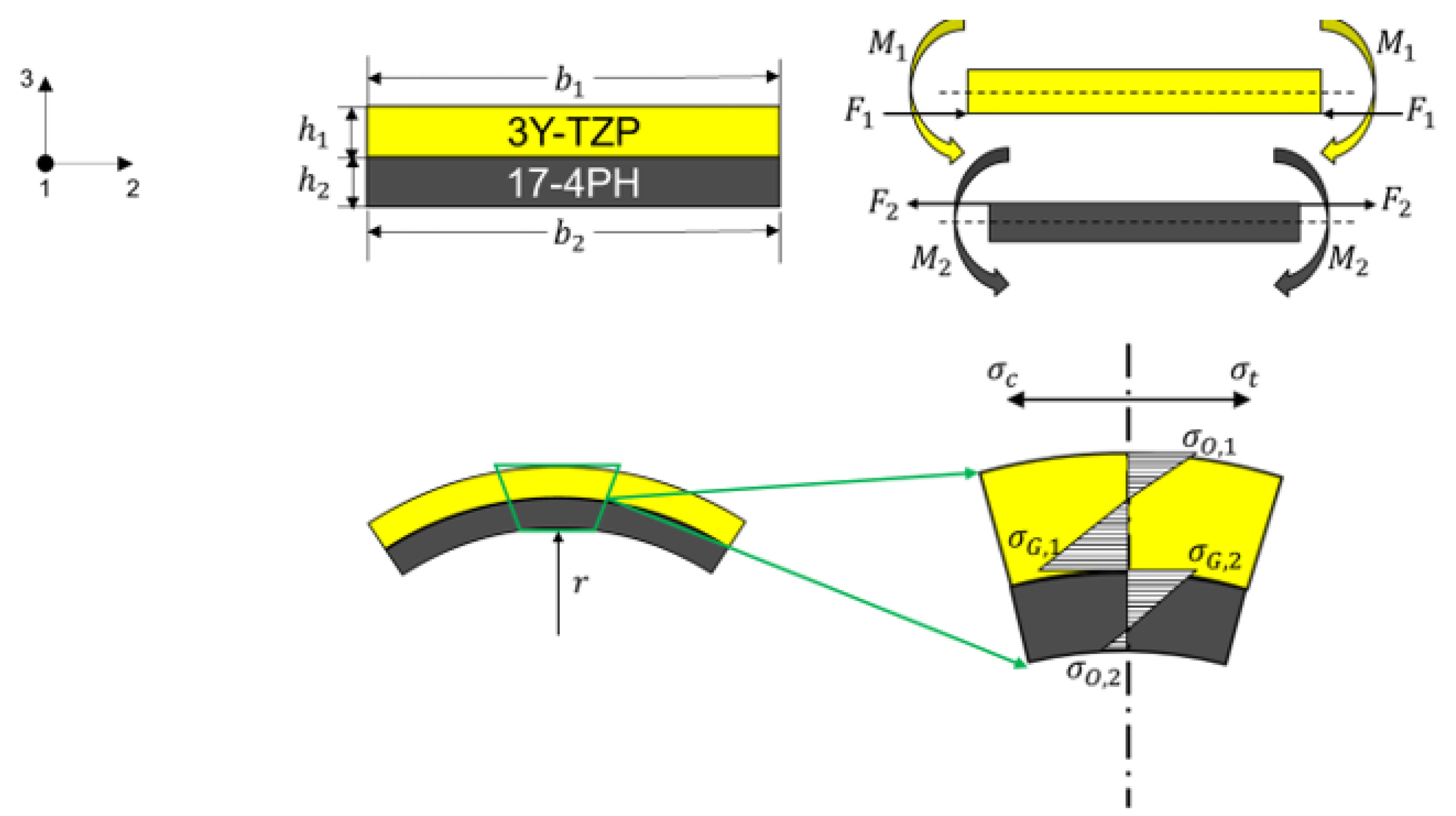
2.4. Analytic Solution for the Curvature and Stress Distribution
3. Results and Discussion for the Analytic Solution and FE Simulation
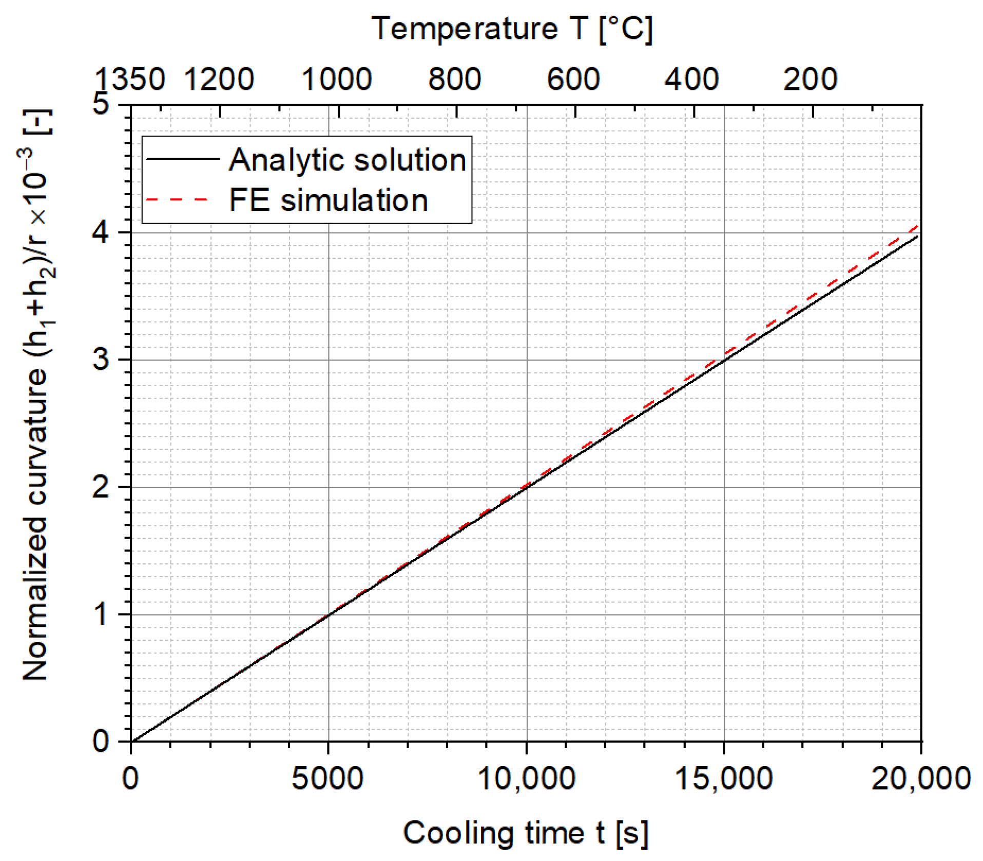
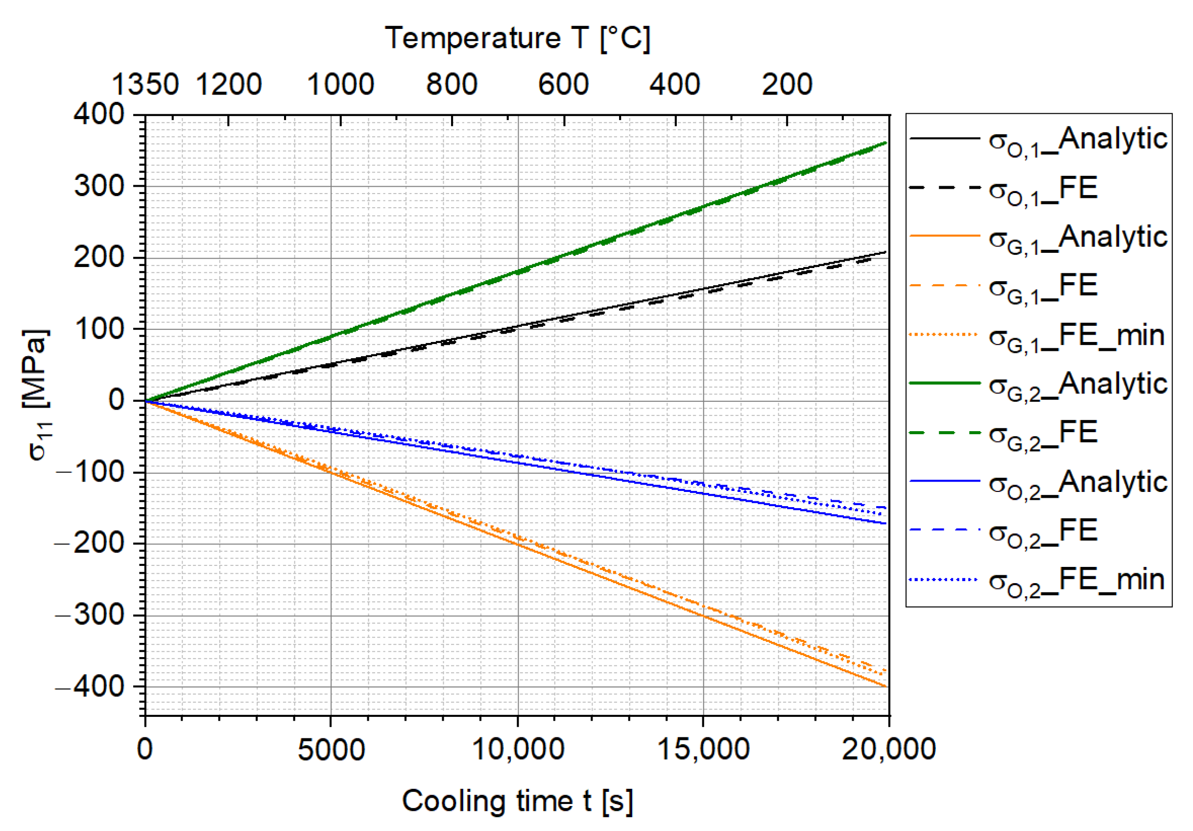
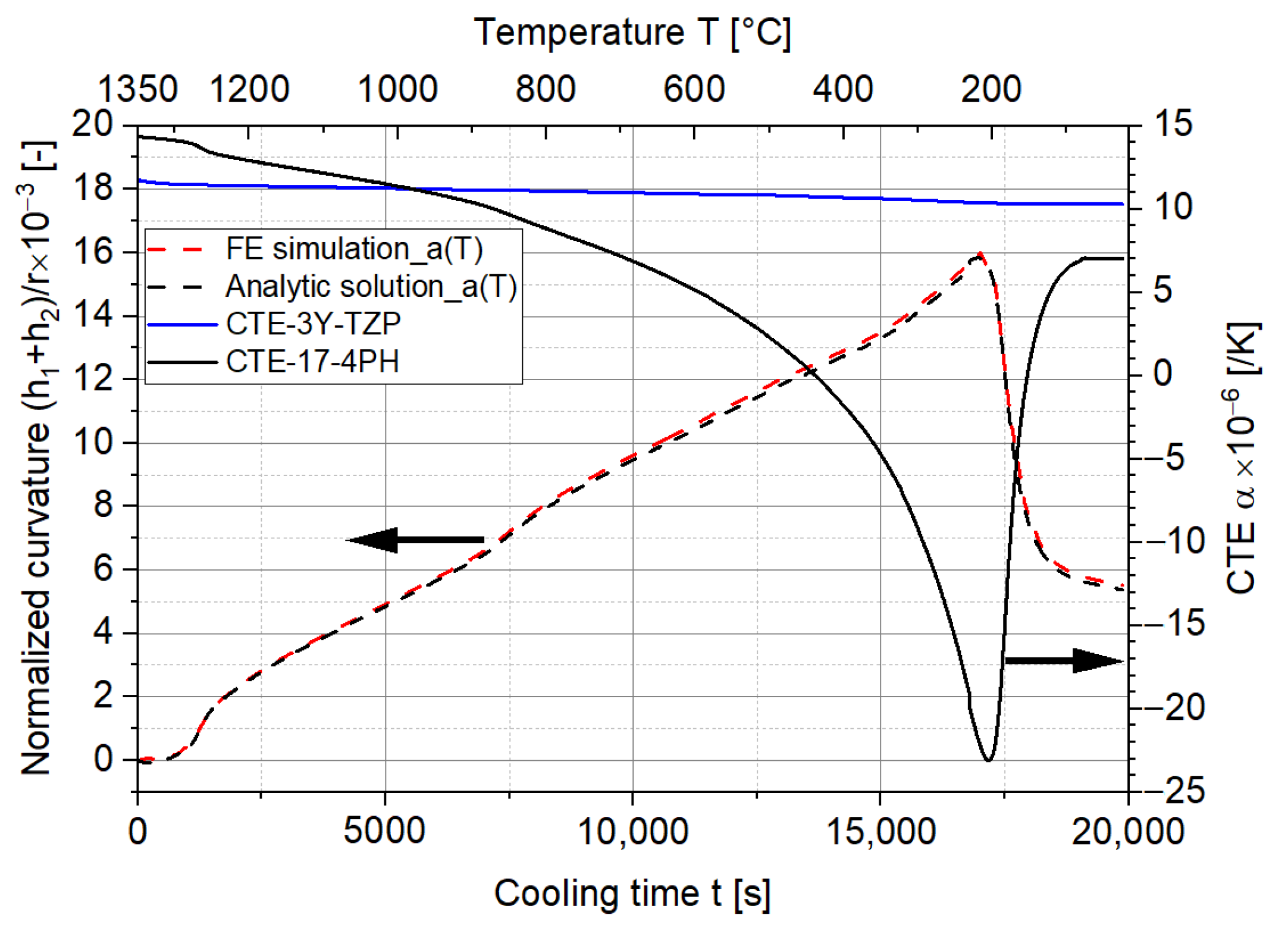
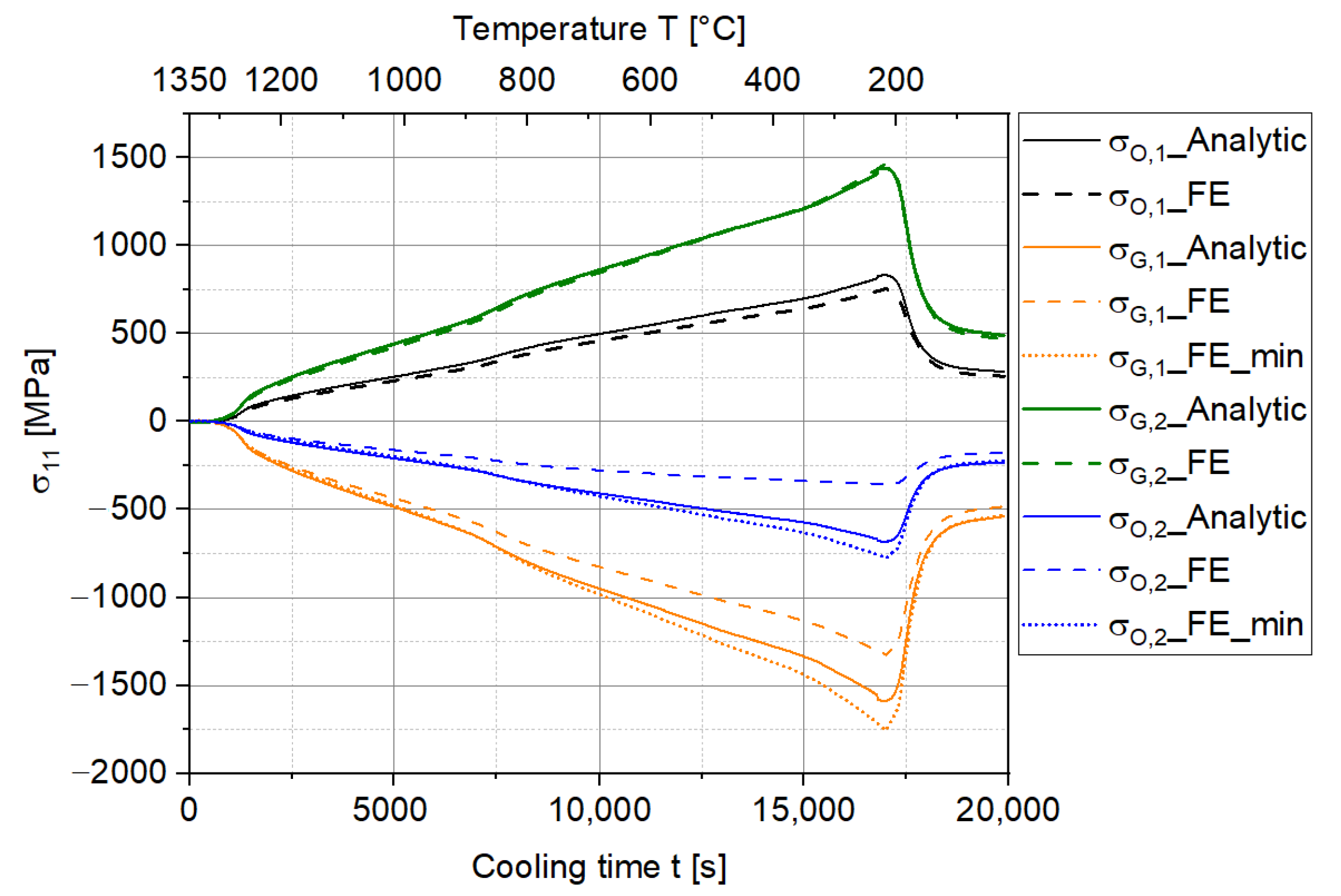
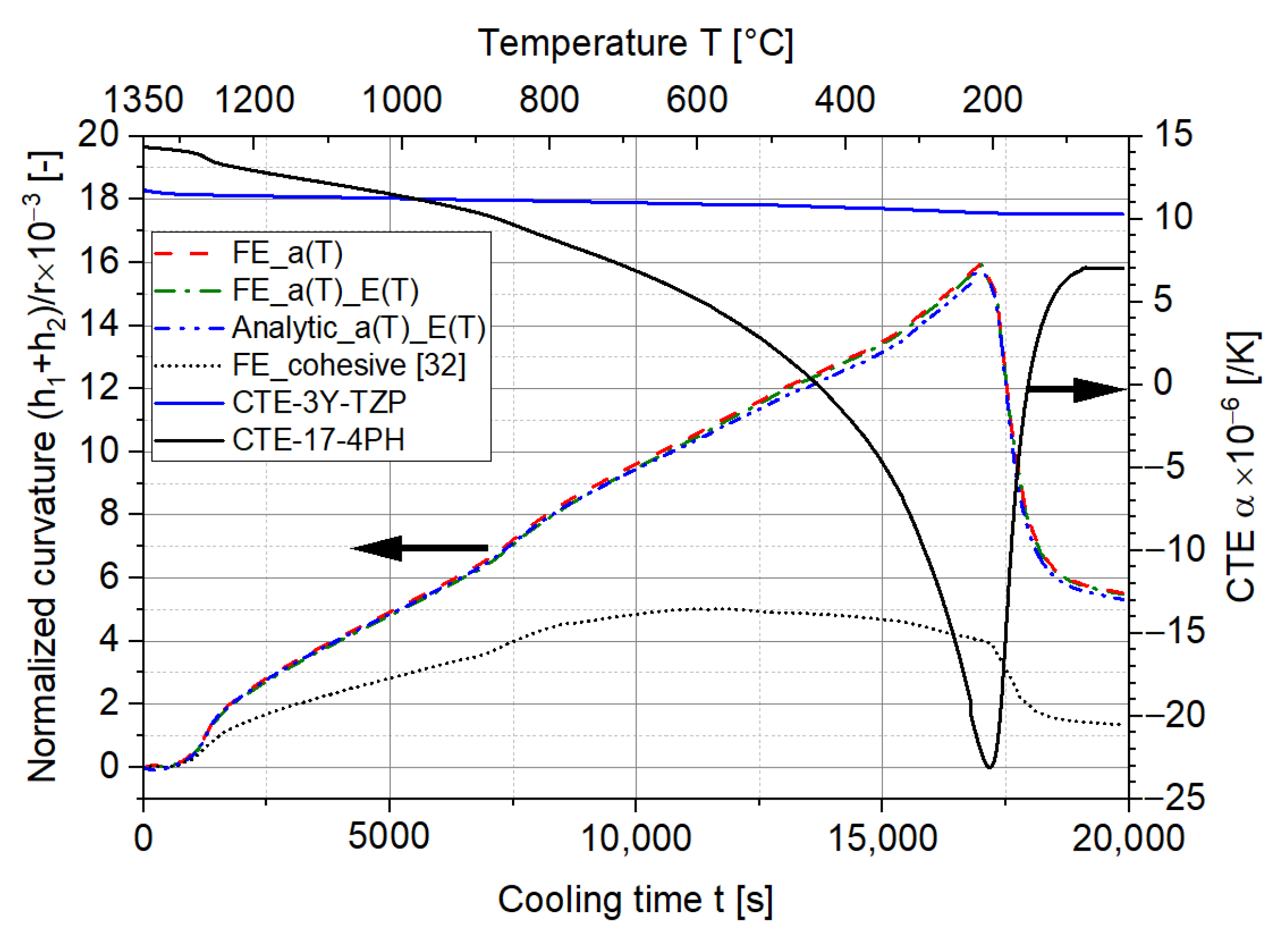
3.1. Comparison of the Analytic Solution and FE Simulation
3.2. Influence of the E Modulus and Cohesive Contact
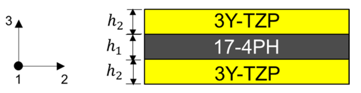
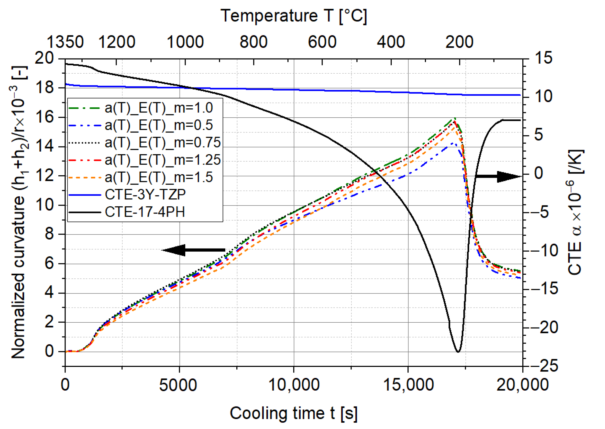
3.3. Influence of Height Ratio
4. Conclusions
- The FE simulation of the curvature of the two-layer MCLs corresponds very well to the analytic solution. Meanwhile, the stress values are generally slightly lower than the analytic solution due to the numerical extrapolation error in the FE simulation.
- The CTE differences have the most significant influence on the curvature and stress distribution of the laminates, whereas the influence of the change in the elastic constants with temperature for the investigated material combination is less pronounced.
- The height ratio also affects the curvature of the two-layer MCLs, and lower curvatures occur when one layer has a much higher or lower thickness than the other.
- The cohesive contact reduces the curvature of the two-layer MCLs considerably due to the energy dissipation mechanism. This provides hints to avoid delamination during the manufacturing of the laminates.
Author Contributions
Funding
Institutional Review Board Statement
Informed Consent Statement
Data Availability Statement
Acknowledgments
Conflicts of Interest
Nomenclature
| CTE | Coefficient of thermal expansion | Width of the cross-section | |
| MCLs | Metal–ceramic laminates | Height of the cross-section | |
| TB | Timoshenko beam | Radius of the curvature | |
| VE | Viscous-elastic | Area of the cross-section | |
| SOFC | Solid oxide fuel cell | Force | |
| FE | Finite element | Normalized curvature | |
| Stress | Layer height ratio | ||
| Strain | Temperature difference | ||
| Young’s modulus | Coefficient of thermal expansion | ||
| Shear modulus | Stress on the top side of the upper layer | ||
| Poisson’s ratio | Stress at the interface of the upper layer | ||
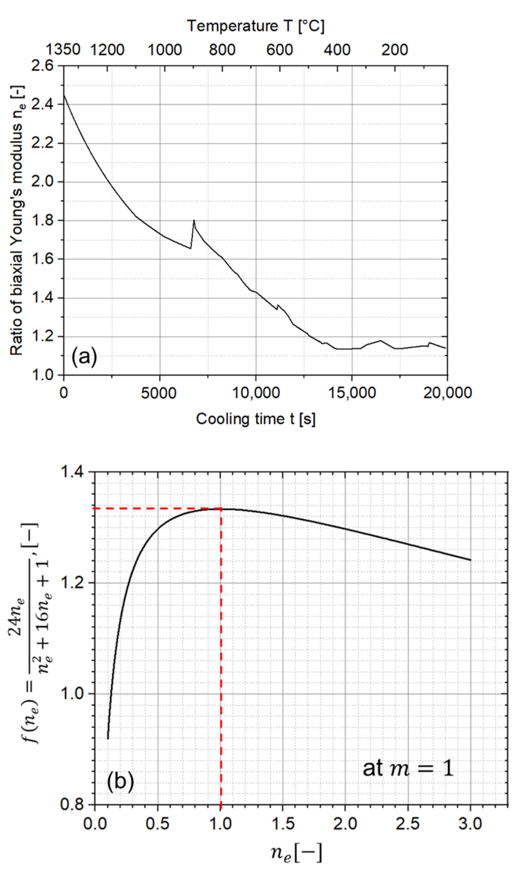
| Biaxial Young’s modulus | Stress at the interface of the bottom layer | ||
| Ratio of biaxial Young’s modulus | Stress on the downside of the bottom layer | ||
| Bending moment | Number of layers | ||
| Moment of inertia |
References
- Munz, D.; Fett, T. Ceramics: Mechanical Properties, Failure Behaviour, Materials Selection, 1st ed.; Springer: Berlin/Heidelberg, Germany, 1999. [Google Scholar]
- Rödel, J.; Kounga, A.B.; Weissenberger-Eibl, M.; Koch, D.; Bierwisch, A.; Rossner, W.; Hoffmann, M.J.; Danzer, R.; Schneider, G. Development of a roadmap for advanced ceramics: 2010–2025. J. Eur. Ceram. Soc. 2009, 29, 1549–1560. [Google Scholar] [CrossRef]
- Bermejo, R.; Deluca, M. Layered Ceramics. In Handbook of Advanced Ceramics; Elsevier: Amsterdam, The Netherlands, 2013; pp. 733–751. [Google Scholar]
- Scheithauer, U.; Schwarzer, E.; Otto, C.; Slawik, T.; Moritz, T.; Michaelis, A. Ceramic and Metal-Ceramic Components with Graded Microstructure. In Ceramic Transactions Series, Advanced and Refractory Ceramics for Energy Conservation and Efficiency; Lin, H.-T., Hemrick, J., Eds.; John Wiley & Sons, Inc.: Hoboken, NJ, USA, 2016; Volume 256, pp. 149–160. [Google Scholar]
- Scheithauer, U.; Slawik, T.; Haderk, K.; Moritz, T.; Michaelis, A. Development of Planar and Cylindrical Refractories with Graded Microstructure. In Proceedings of the Unified International Technical Conference on Refractories (UNITECR) 2013, Victoria, Australia, 10–13 September 2013. [Google Scholar]
- Bermejo, R.; Torress, Y.; Sanchez-Herrencia, A.; Baudín, C.; Anglada, M.; Llanes, L. Residual stresses, strength and toughness of laminates with different layer thickness ratios. Acta Mater. 2006, 54, 4745–4757. [Google Scholar] [CrossRef]
- Cai, P.Z.; Green, D.J.; Messing, G.L. Constrained Densification of Alumina/Zirconia Hybrid Laminates, I: Experimental Observations of Processing Defects. J. Am. Ceram. Soc. 1997, 80, 1929–1939. [Google Scholar] [CrossRef]
- Largiller, G.; Bouvard, D.; Carry, C.P.; Gabriel, A.; Müller, J.; Staab, T. Deformation and cracking during sintering of bimaterial components processed from ceramic and metal powder mixes. Part I: Experimental investigation. Mech. Mater. 2012, 53, 123–131. [Google Scholar] [CrossRef]
- Pascual-Herrero, J. Influence of Residual Stresses on Strength and Toughness of an Alumina/Alumina-Zirconia Laminate. Ph.D. Thesis, University of Leoben, Leoben, Austria, May 2007. [Google Scholar]
- Dourandish, M.; Simchi, A.; Tamjid Shabestary, E.; Hartwig, T. Pressureless Sintering of 3Y-TZP/Stainless-Steel Composite Layers. 11 August 2020. Available online: http://arxiv.org/pdf/2008.02658v1 (accessed on 28 August 2022).
- Slawik, T.; Günther, A.; Moritz, T.; Michaelis, A. Co-Sintering behaviour of zirconia-ferritic steel composites. AIMS Mater. Sci. 2016, 3, 1160–1176. [Google Scholar] [CrossRef]
- Slawik, T.; Bergner, A.; Puschmann, R.; Franke, P.; Raethel, J.; Behnisch, T.; Scholl, R.; Berger, L.-M.; Moritz, T.; Zelm, R.; et al. Metal-Ceramic Layered Materials and Composites Manufactured Using Powder Techniques. Adv. Eng. Mater. 2014, 16, 1293–1302. [Google Scholar] [CrossRef]
- Timoshenko, S. Analysis of Bi-Metal Thermostats. J. Opt. Soc. Am. 1925, 11, 233. [Google Scholar] [CrossRef]
- Swain, M.V. Unstable cracking (chipping) of veneering porcelain on all-ceramic dental crowns and fixed partial dentures. Acta Biomater. 2009, 5, 1668–1677. [Google Scholar] [CrossRef] [PubMed]
- Hsueh, C.-H.; Luttrell, C.R.; Becher, P.F. Analyses of multilayered dental ceramics subjected to biaxial flexure tests. Dent. Mater. 2006, 22, 460–469. [Google Scholar] [CrossRef]
- Hsueh, C.H.; Thompson, G.A.; Jadaan, O.M.; Wereszczak, A.A.; Becher, P.F. Analyses of layer-thickness effects in bilayered dental ceramics subjected to thermal stresses and ring-on-ring tests. Dent. Mater. 2008, 24, 9–17. [Google Scholar] [CrossRef]
- Yu, Y.; Ashcroft, I.A.; Swallowe, G. An experimental investigation of residual stresses in an epoxy–steel laminate. Int. J. Adhes. Adhes. 2006, 26, 511–519. [Google Scholar] [CrossRef]
- Jumbo, F.S.; Ashcroft, I.A.; Crocombe, A.D.; Abdel Wahab, M. Thermal residual stress analysis of epoxy bi-material laminates and bonded joints. Int. J. Adhes. Adhes. 2010, 30, 523–538. [Google Scholar] [CrossRef]
- Green, D.J.; Cai, P.Z.; Messing, G.L. Residual stresses in alumina–zirconia laminates. J. Eur. Ceram. Soc. 1999, 19, 2511–2517. [Google Scholar] [CrossRef]
- Cai, P.Z.; Messing, G.L.; Green, D.J. Determination of the Mechanical Response of Sintering Compacts by Cyclic Loading Dilatometry. J. Am. Ceram. Soc. 1997, 80, 445–452. [Google Scholar] [CrossRef]
- Ravi, D.; Green, D.J. Sintering stresses and distortion produced by density differences in bi-layer structures. J. Eur. Ceram. Soc. 2006, 26, 17–25. [Google Scholar] [CrossRef]
- Chang, J.; Guillon, O.; Rödel, J.; Kang, S.-J.L. Characterization of warpage behaviour of Gd-doped ceria/NiO–yttria stabilized zirconia bi-layer samples for solid oxide fuel cell application. J. Power Sources 2008, 185, 759–764. [Google Scholar] [CrossRef]
- Reynier, T.; Bouvard, D.; Carry, C.P.; Laucournet, R. Co-Sintering of an Anode-Supported SOFC Based on Scandia Stabilized Zirconia Electrolyte. In Advances in Sintering Science and Technology II: Ceramic Transactions; The American Ceramic Society: Columbus, OH, USA, 2012; pp. 91–99. [Google Scholar]
- Ollagnier, J.-B.; Guillon, O.; Rödel, J. Constrained Sintering of a Glass Ceramic Composite: I. Asymmetric Laminate. J. Am. Ceram. Soc. 2010, 93, 74–81. [Google Scholar] [CrossRef]
- Ni, D.-W.; Esposito, V.; Schmidt, C.G.; Molla, T.T.; Andersen, K.B.; Kaiser, A.; Ramousse, S.; Pryds, N. Camber Evolution and Stress Development of Porous Ceramic Bilayers During Co-Firing. J. Am. Ceram. Soc. 2013, 96, 972–978. [Google Scholar] [CrossRef]
- Wu, K.; Scheler, S.; Park, H.-S.; Willert-Porada, M. Pressureless sintering of ZrO2–ZrSiO4/NiCr functionally graded materials with a shrinkage matching process. J. Eur. Ceram. Soc. 2013, 33, 1111–1121. [Google Scholar] [CrossRef]
- Günther, A.; Moritz, T.; Mühle, U. Microstructure and Interface Characteristics of 17-4PH/YSZ Components after Co-Sintering and Hydrothermal Corrosion. Ceramics 2020, 3, 245–257. [Google Scholar] [CrossRef]
- EN 15335:2007; Advanced Technical Ceramics-Ceramic Composites-Determination of Elastic Properties by Resonant Beam Method up to 2000 °C. Beuth Verlag GmbH: Berlin, Germany, 2007.
- ASTM E1876-22; Test Method for Dynamic Youngs Modulus, Shear Modulus, and Poissons Ratio by Impulse Excitation of Vibration. ASTM International: West Conshohocken, PA, USA, 2022.
- Matsui, K.; Yoshida, H.; Ikuhara, Y. Nanocrystalline, ultra-degradation-resistant zirconia: Its grain boundary nanostructure and nanochemistry. Sci. Rep. 2014, 4, 4758. [Google Scholar] [CrossRef] [PubMed]
- Chartier, T.; Merle, D.; Besson, J.L. Laminar ceramic composites. J. Eur. Ceram. Soc. 1995, 15, 101–107. [Google Scholar] [CrossRef]
- Khoramishad, H. Modelling Fatigue Damage in Adhesively Bonded Joints. Ph.D. Thesis, University of Surrey, Guildford, UK, May 2010. [Google Scholar]


| Materials | FE Simulation | ||
|---|---|---|---|
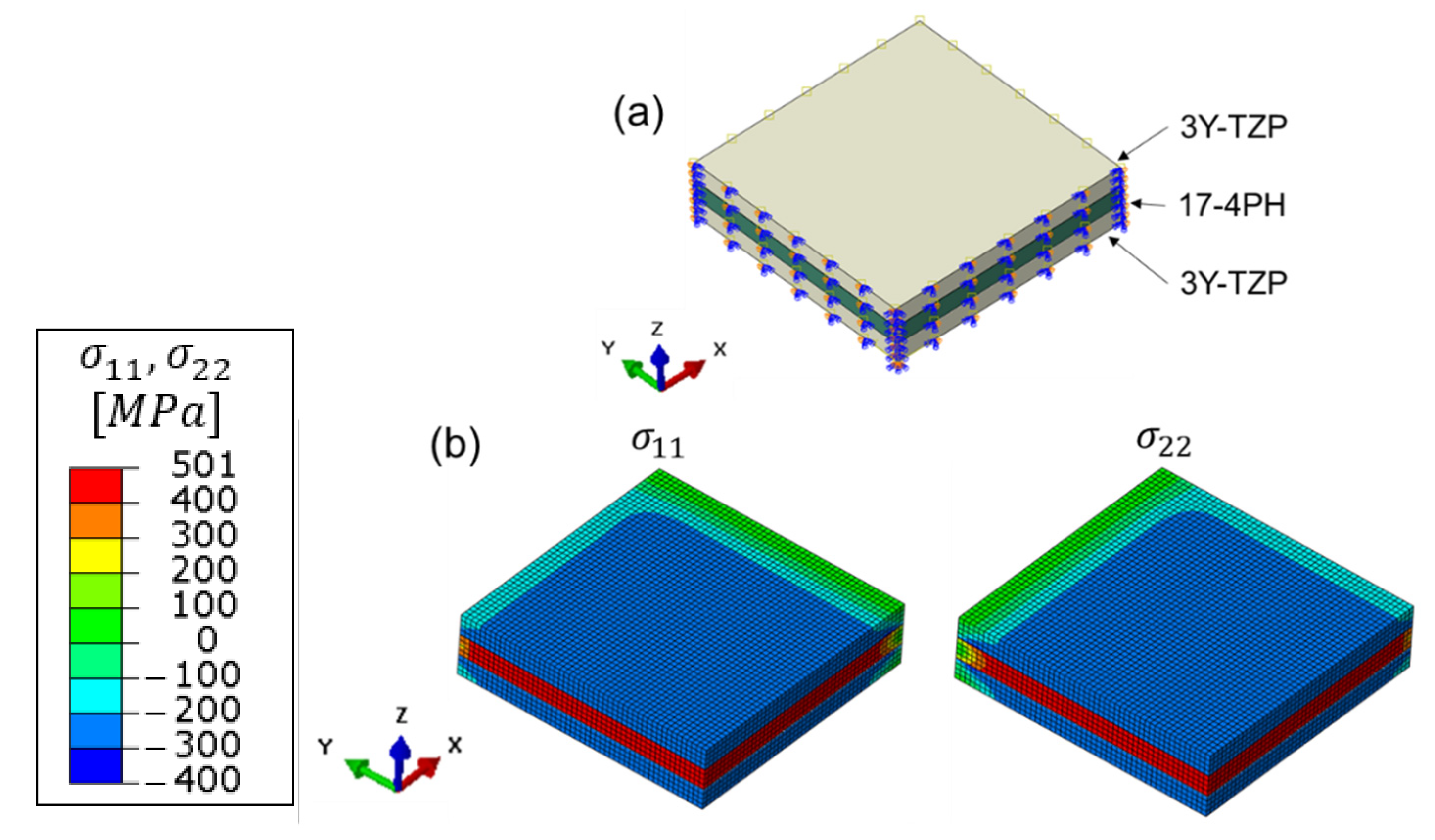
| 3Y-TZP | −247 | −227 | −227 |
| 17-4PH | 494 | 456 | 456 |
Publisher’s Note: MDPI stays neutral with regard to jurisdictional claims in published maps and institutional affiliations. |
© 2022 by the authors. Licensee MDPI, Basel, Switzerland. This article is an open access article distributed under the terms and conditions of the Creative Commons Attribution (CC BY) license (https://creativecommons.org/licenses/by/4.0/).
Share and Cite
Liu, C.; Günther, A.; Deng, Y.; Kaletsch, A.; Herrmann, M.; Broeckmann, C. Investigation on the Curvature and Stress Distribution of Laminates Based on an Analytic Solution and FE Simulation. Materials 2022, 15, 6458. https://doi.org/10.3390/ma15186458
Liu C, Günther A, Deng Y, Kaletsch A, Herrmann M, Broeckmann C. Investigation on the Curvature and Stress Distribution of Laminates Based on an Analytic Solution and FE Simulation. Materials. 2022; 15(18):6458. https://doi.org/10.3390/ma15186458
Chicago/Turabian StyleLiu, Chao, Anne Günther, Yuanbin Deng, Anke Kaletsch, Mathias Herrmann, and Christoph Broeckmann. 2022. "Investigation on the Curvature and Stress Distribution of Laminates Based on an Analytic Solution and FE Simulation" Materials 15, no. 18: 6458. https://doi.org/10.3390/ma15186458
APA StyleLiu, C., Günther, A., Deng, Y., Kaletsch, A., Herrmann, M., & Broeckmann, C. (2022). Investigation on the Curvature and Stress Distribution of Laminates Based on an Analytic Solution and FE Simulation. Materials, 15(18), 6458. https://doi.org/10.3390/ma15186458